admm

Lecture given for the course ELEC5470/IEDA6100A Convex Optimization at HKUST.

Transcript

1. Alternating Direction Method of Multipliers ELEC5470/IEDA6100A - Convex Optimization a talk by Vinícius and Prof. Daniel Palomar The Hong Kong University of Science and Technology December, 2020
2. Contents 1. Introduction Optimization algorithms, motivation 2. Alternating Direction Method of Multipliers The basics 3. Practical Examples Robust PCA and Graphical Lasso
3. 1/28 Whyuseoptimizationalgorithms?
4. Motivations 2/28 large-scale optimization machine learning/statistics with huge datasets computer vision descentralized optimization entities/agents/threads coordinate to solve a large problem by passing small messages
5. Optimization Algorithms 3/28 Gradient Descent Newton Interior Point Methods (IPM) Block Coordinate Descent (BCD) Majorization-Minimization (MM) Block Majorization-Minimization (BMM) Successive Convex Approximation (SCA)
6. Optimization Algorithms 3/28 Gradient Descent Newton Interior Point Methods (IPM) Block Coordinate Descent (BCD) Majorization-Minimization (MM) Block Majorization-Minimization (BMM) Successive Convex Approximation (SCA) ...
7. Optimization Algorithms 3/28 Gradient Descent Newton Interior Point Methods (IPM) Block Coordinate Descent (BCD) Majorization-Minimization (MM) Block Majorization-Minimization (BMM) Successive Convex Approximation (SCA) ... Alternating Direction Method of Multipliers (ADMM)
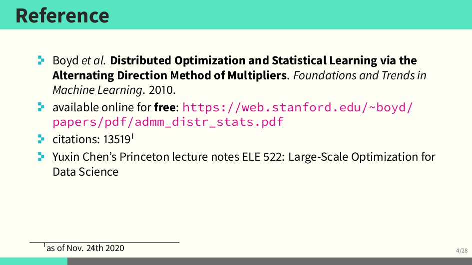
8. Reference 4/28 Boyd et al. Distributed Optimization and Statistical Learning via the Alternating Direction Method of Multipliers. Foundations and Trends in Machine Learning. 2010. available online for free: https://web.stanford.edu/~boyd/ papers/pdf/admm_distr_stats.pdf citations: 135191 Yuxin Chen’s Princeton lecture notes ELE 522: Large-Scale Optimization for Data Science 1as of Nov. 24th 2020
9. Dual Problem 5/28 convex equality constrained optimization problem minimize x f(x) subject to Ax = b Lagrangian: L(x, y) = f(x) + y⊤(Ax − b) dual function: g(y) = inf x L(x, y) dual problem: maximize y g(y) recover: x⋆ = argmin x L(x, y⋆)
10. 6/28 DualAscent
11. Dual Ascent 7/28 gradient method for dual problem: yk+1 = yk + ρk∇g(yk) ∇g(yk) = Axk+1 − b, where xk+1 = arg min x L(x, yk) dual ascent method is xk+1 := arg min x L(x, yk) yk+1 := yk + ρk Axk+1 − b
12. Dual Ascent 7/28 gradient method for dual problem: yk+1 = yk + ρk∇g(yk) ∇g(yk) = Axk+1 − b, where xk+1 = arg min x L(x, yk) dual ascent method is xk+1 := arg min x L(x, yk) yk+1 := yk + ρk Axk+1 − b why?
13. 8/28 DualDecomposition
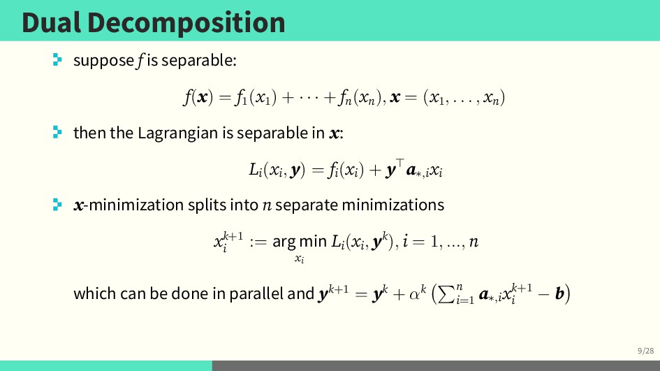
14. Dual Decomposition 9/28 suppose f is separable: f(x) = f1 (x1 ) + · · · + fn (xn ), x = (x1 , . . . , xn ) then the Lagrangian is separable in x: Li (xi , y) = fi (xi ) + y⊤a∗,i xi x-minimization splits into n separate minimizations xk+1 i := arg min xi Li (xi , yk), i = 1, ..., n which can be done in parallel and yk+1 = yk + αk n i=1 a∗,i xk+1 i − b
15. Optimization Problem 10/28 minimize x, z f(x) + g(z) subject to Ax + Bz = c (1) variables: x ∈ Rn and z ∈ Rm parameters: A ∈ Rp×n, B ∈ Rp×m, and c ∈ Rp optimal value: p⋆ = inf x,z {f(x) + g(z) : Ax + Bz = c}
16. 11/28 AugmentedLagrangianMethod
17. Augmented Lagrangian Method 12/28 Augmented Lagrangian: Lρ (x, z, y) = f(x) + g(z) + ⟨y, Ax + Bz − c⟩ Lagrangian + ρ 2 ∥Ax + Bz − c∥2 F ALM consists of the iterations: xk+1, zk+1 := arg min x,z Lρ (x, z, yk) // primal update yk+1 := yk + ρ Axk+1 + Bzk+1 − c // dual update ρ > 0 is a penalty hyperparameter
18. Issues with Augmented Lagrangian Method 13/28 the primal step is often expensive to solve – as expensive as solving the original problem minimization of x and z has to be done jointly
19. 14/28 AlternatingDirection MethodofMultipliers
20. Alternating Direction Method of Multipliers 15/28 Augmented Lagrangian: Lρ (x, z, y) = f(x) + g(z) + ⟨y, Ax + Bz − c⟩ Lagrangian + ρ 2 ∥Ax + Bz − c∥2 F ADMM consists of the iterations: xk+1 := arg min x Lρ (x, zk, yk) zk+1 := arg min z Lρ (xk+1, z, yk) yk+1 := yk + ρ Axk+1 + Bzk+1 − c ρ > 0 is a penalty hyperparameter
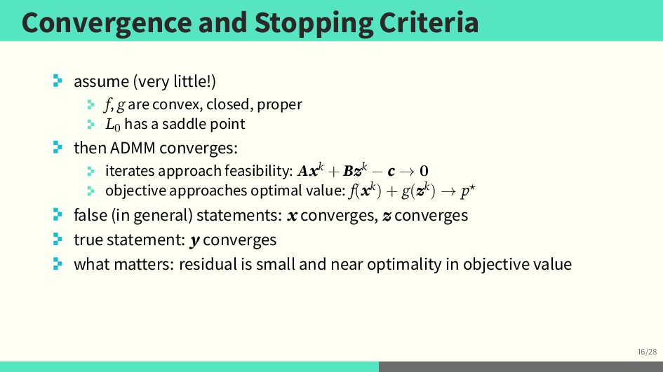
21. Convergence and Stopping Criteria 16/28 assume (very little!) f, g are convex, closed, proper L0 has a saddle point then ADMM converges: iterates approach feasibility: Axk + Bzk − c → 0 objective approaches optimal value: f(xk) + g(zk) → p⋆ false (in general) statements: x converges, z converges true statement: y converges what matters: residual is small and near optimality in objective value
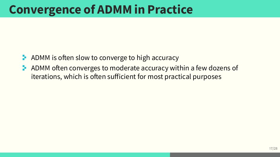
22. Convergence of ADMM in Practice 17/28 ADMM is often slow to converge to high accuracy ADMM often converges to moderate accuracy within a few dozens of iterations, which is often sufficient for most practical purposes
23. 18/28 PracticalExamples
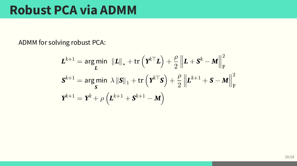
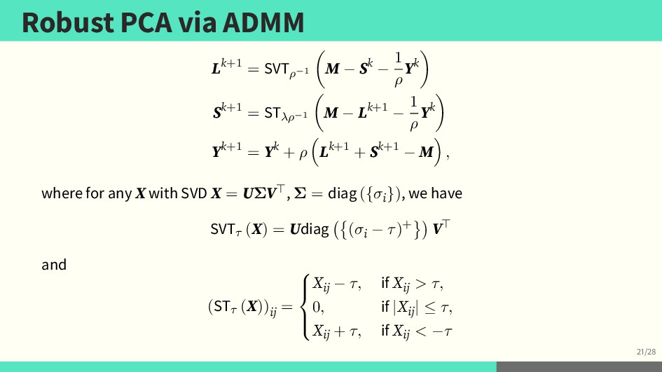
24. Robust PCA (Candes et al. ’08) 19/28 We would like to model a data matrix M as low-rank plus sparse components: minimize L, S ∥L∥∗ + λ ∥S∥1 subject to L + S = M where ∥L∥ ∗ := n i=1 σi (L) is the nuclear norm and ∥S∥ 1 := i,j |Sij | is the entrywise ℓ1 -norm
25. Robust PCA via ADMM 20/28 ADMM for solving robust PCA: Lk+1 = arg min L ∥L∥∗ + tr Yk⊤L + ρ 2 L + Sk − M 2 F Sk+1 = arg min S λ ∥S∥1 + tr Yk⊤S + ρ 2 Lk+1 + S − M 2 F Yk+1 = Yk + ρ Lk+1 + Sk+1 − M
26. Robust PCA via ADMM 21/28 Lk+1 = SVTρ−1 M − Sk − 1 ρ Yk Sk+1 = STλρ−1 M − Lk+1 − 1 ρ Yk Yk+1 = Yk + ρ Lk+1 + Sk+1 − M , where for any X with SVD X = UΣV⊤, Σ = diag ({σi}), we have SVTτ (X) = Udiag (σi − τ)+ V⊤ and (STτ (X))ij =      Xij − τ, if Xij > τ, 0, if |Xij| ≤ τ, Xij + τ, if Xij < −τ
27. Graphical Lasso 22/28 Precision matrix estimation from Gaussian samples: minimize Θ −log det Θ + ⟨Θ, S⟩ neg. log likelihood +λ ∥Θ∥ 1 subject to Θ ≻ 0 Or equivalently, using a slack variable Ψ = Θ minimize Θ,Ψ −log det Θ + ⟨Θ, S⟩ neg. log likelihood +λ ∥Ψ∥ 1 subject to Θ ≻ 0, Θ = Ψ
28. Graphical Lasso via ADMM 23/28 Θk+1 = arg min Θ≻0 − log det Θ + ⟨Θ, S + Yk⟩ + ρ 2 Θ − Ψk 2 F Ψk+1 = arg min Ψ λ ∥Ψ∥1 − ⟨Ψ, Yk⟩ + ρ 2 Θk − Ψ 2 F Yk+1 = Yk + ρ Θk+1 − Ψk+1
29. Graphical Lasso via ADMM 24/28 Θk+1 = Fρ Ψk − 1 ρ Yk + S Ψk+1 = STλρ−1 Θk+1 + 1 ρ Yk Yk+1 = Yk + ρ Θk+1 − Ψk+1 where Fρ (X) := 1 2 Udiag λi + λ2 i + 4 ρ U⊤, for X = UΛU⊤.
30. Network of stocks via Graphical Lasso 25/28
31. Network of stocks via Graphical Lasso 26/28 90 100 110 120 130 140 150 0 100 200 300 400 CPU time [seconds] Lagrangian 0 2 4 6 8 0 100 200 300 400 CPU time [seconds] ||sl|| 2 2
32. Conclusion 27/28 ADMM is a versatile/flexible optimization framework may not be the best for a specific case, but often performs well in practice convergence often needs to be proved in a case-by-case scenario
33. 28/28 Questions?