systems Supported by NNSA Stewardship Science Graduate Fellowship J.S. Moreland, J.E. Bernhard, S.A. Bass | April 6, 2017 Correlations and Fluctuations in p+A and A+A Collisions April 6, 2017 1 / 15
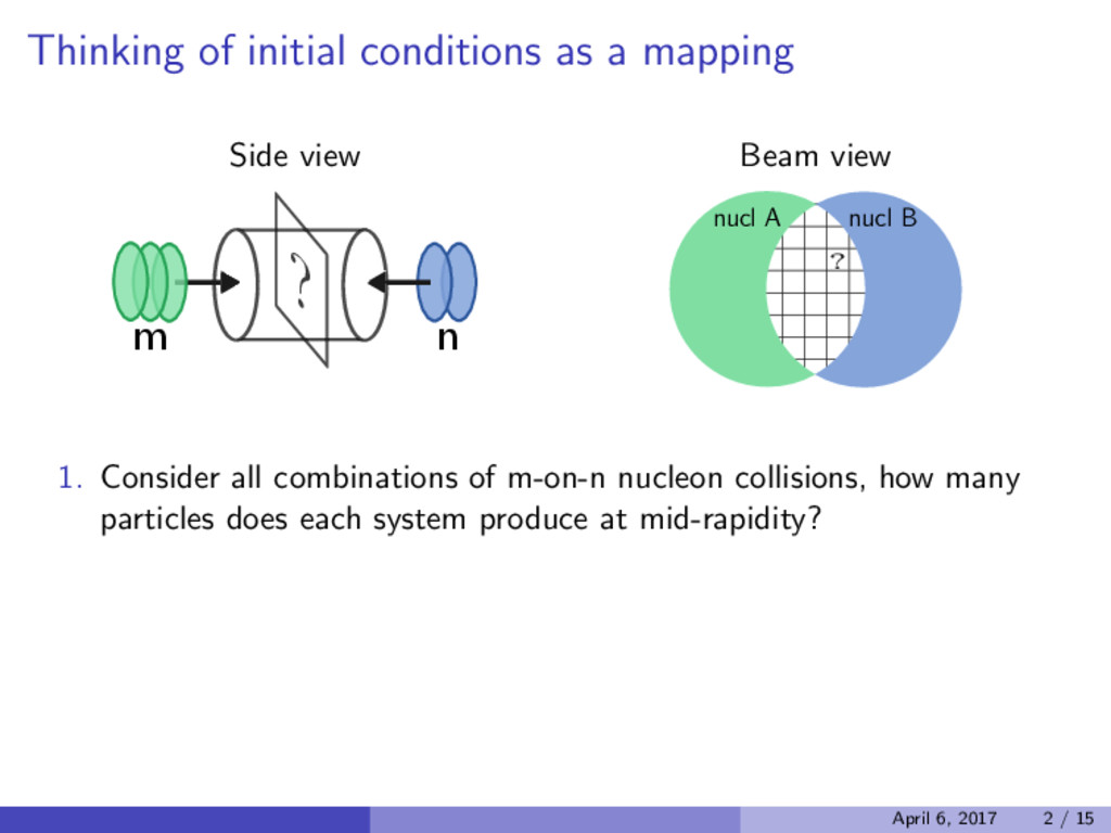
m n Beam view nucl A nucl B ? 1. Consider all combinations of m-on-n nucleon collisions, how many particles does each system produce at mid-rapidity? April 6, 2017 2 / 15
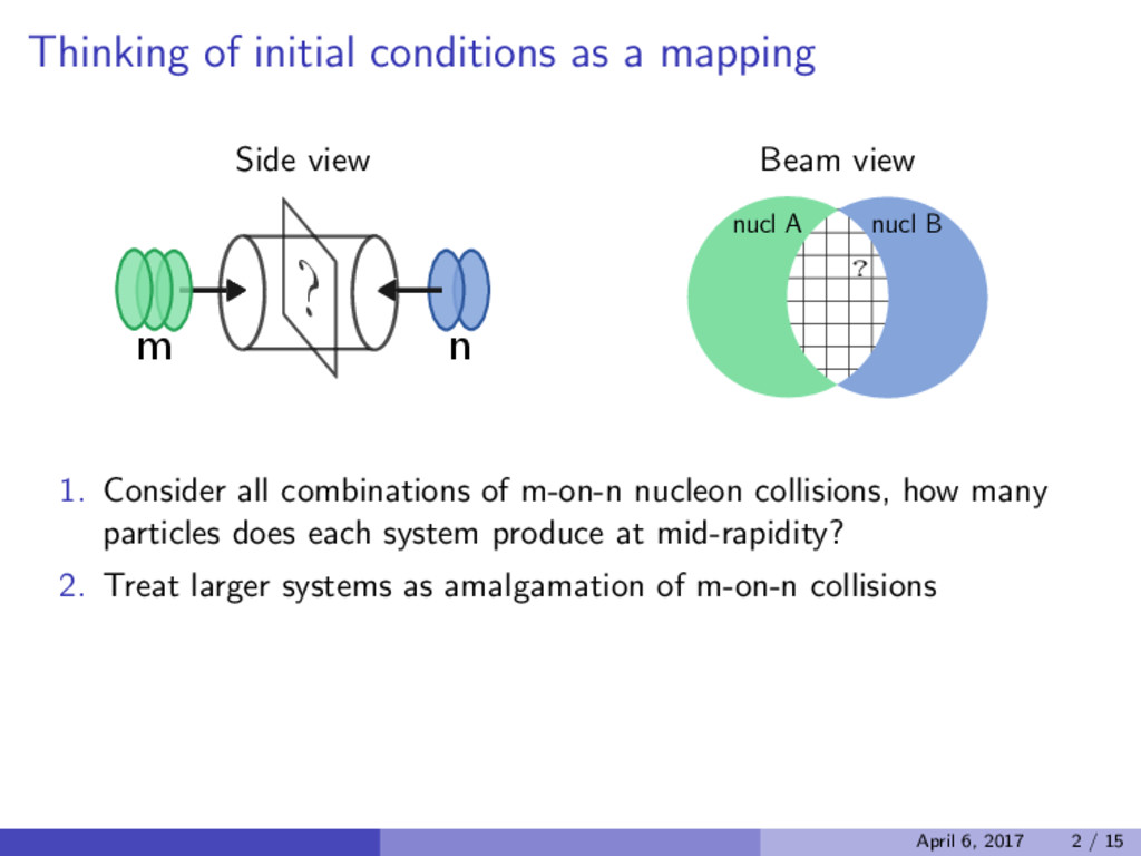
m n Beam view nucl A nucl B ? 1. Consider all combinations of m-on-n nucleon collisions, how many particles does each system produce at mid-rapidity? 2. Treat larger systems as amalgamation of m-on-n collisions April 6, 2017 2 / 15
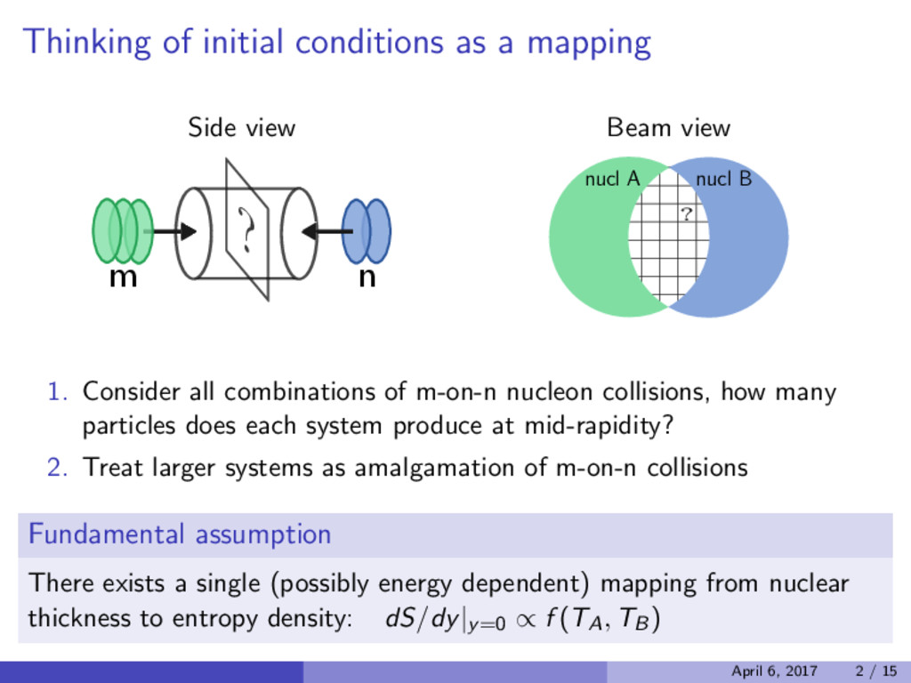
m n Beam view nucl A nucl B ? 1. Consider all combinations of m-on-n nucleon collisions, how many particles does each system produce at mid-rapidity? 2. Treat larger systems as amalgamation of m-on-n collisions Fundamental assumption There exists a single (possibly energy dependent) mapping from nuclear thickness to entropy density: dS/dy|y=0 ∝ f (TA, TB) April 6, 2017 2 / 15
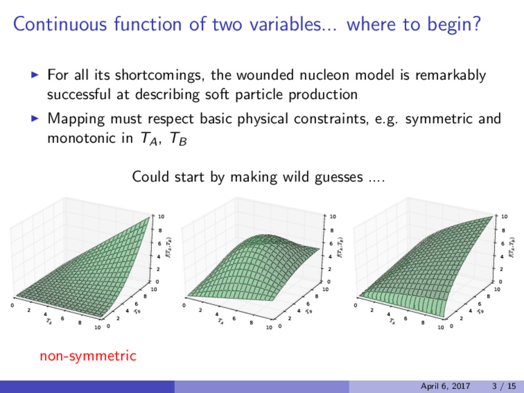
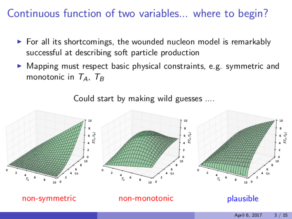
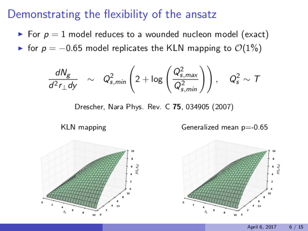
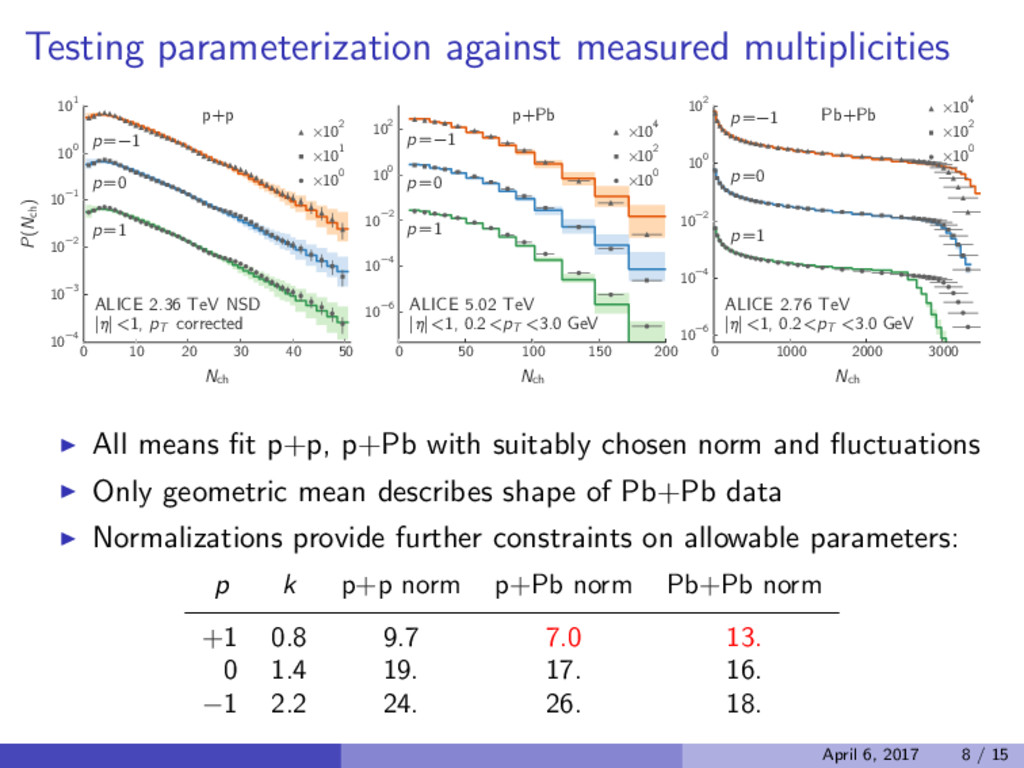
its shortcomings, the wounded nucleon model is remarkably successful at describing soft particle production Mapping must respect basic physical constraints, e.g. symmetric and monotonic in TA, TB April 6, 2017 3 / 15
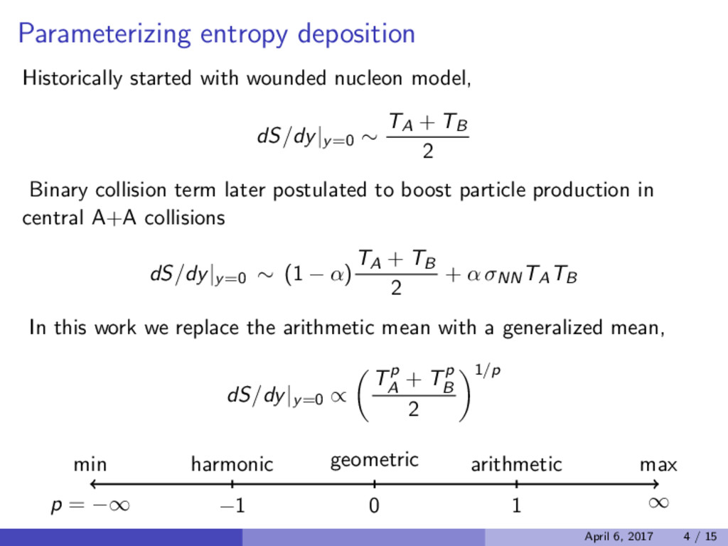
∼ TA + TB 2 Binary collision term later postulated to boost particle production in central A+A collisions dS/dy|y=0 ∼ (1 − α) TA + TB 2 + α σNNTATB April 6, 2017 4 / 15
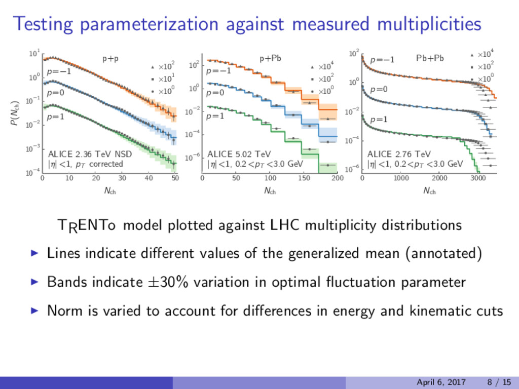
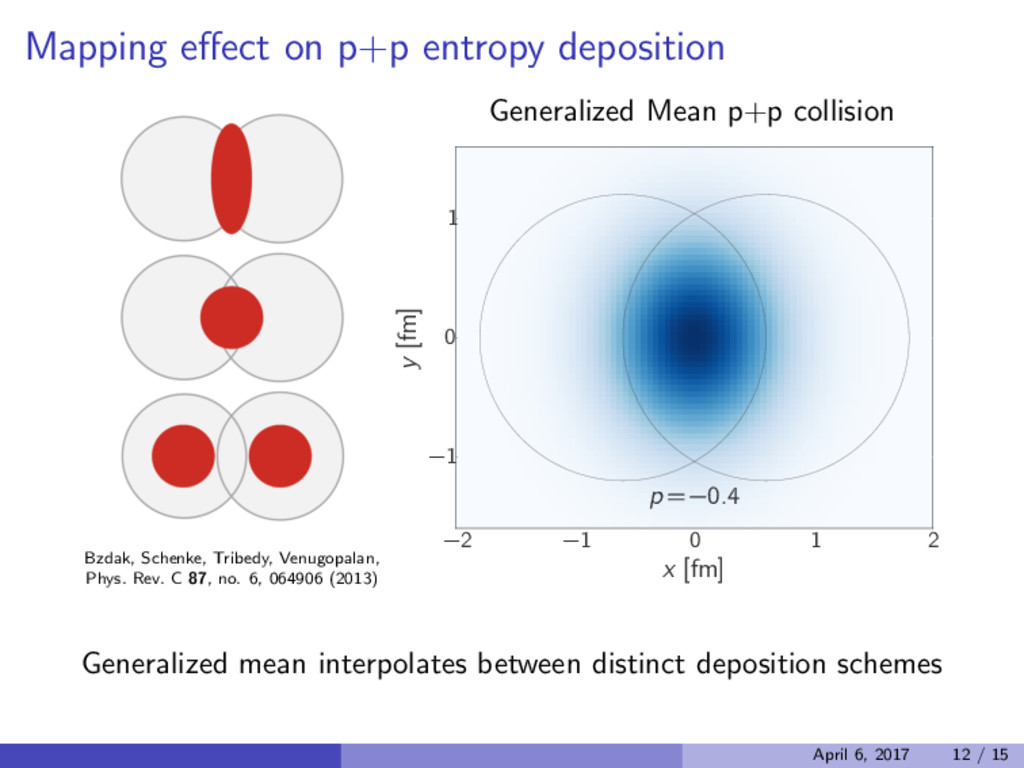
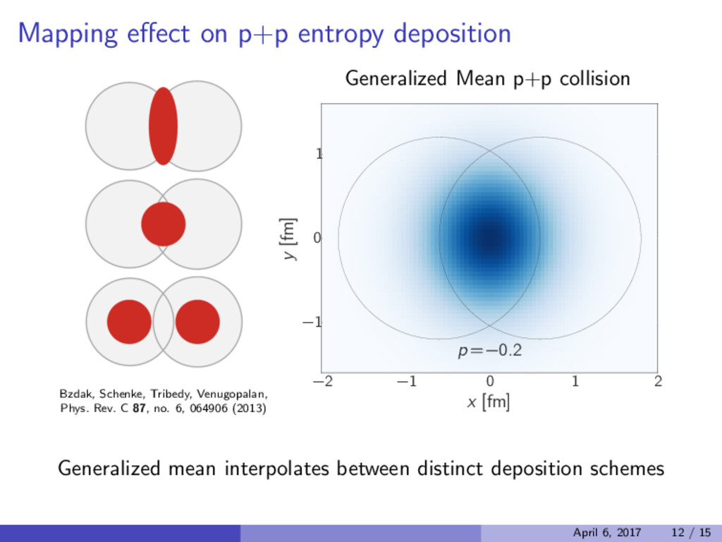
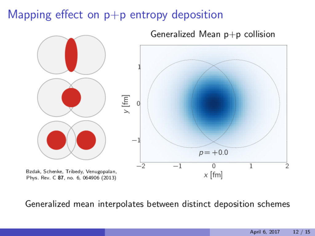
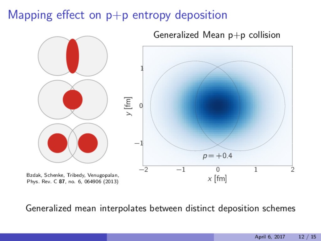
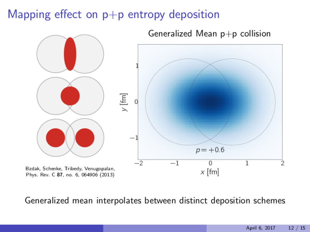
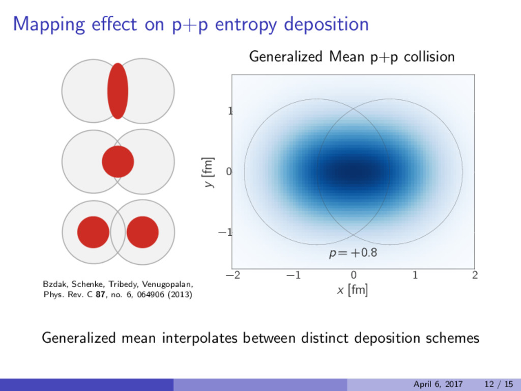
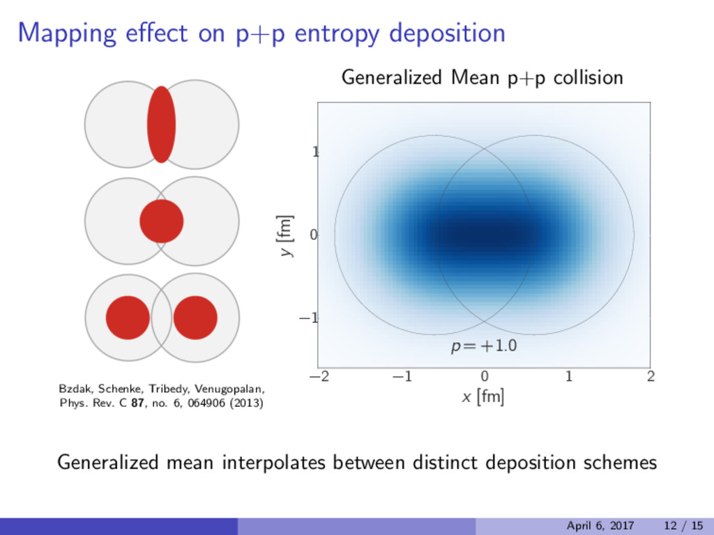
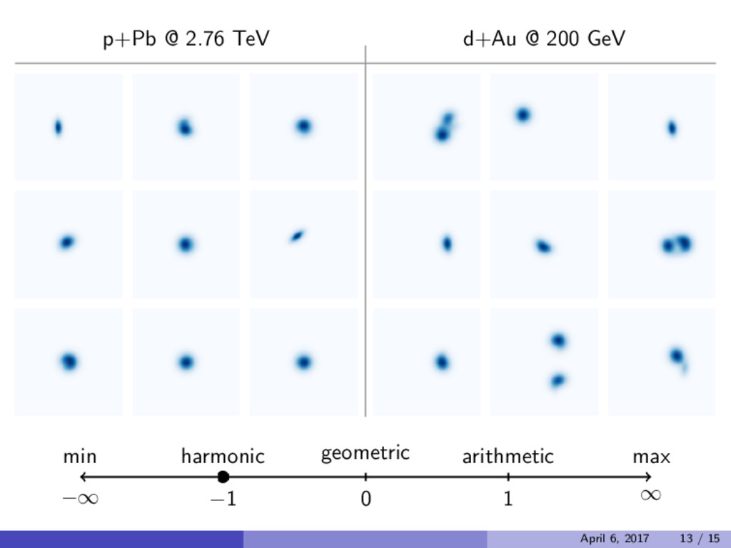
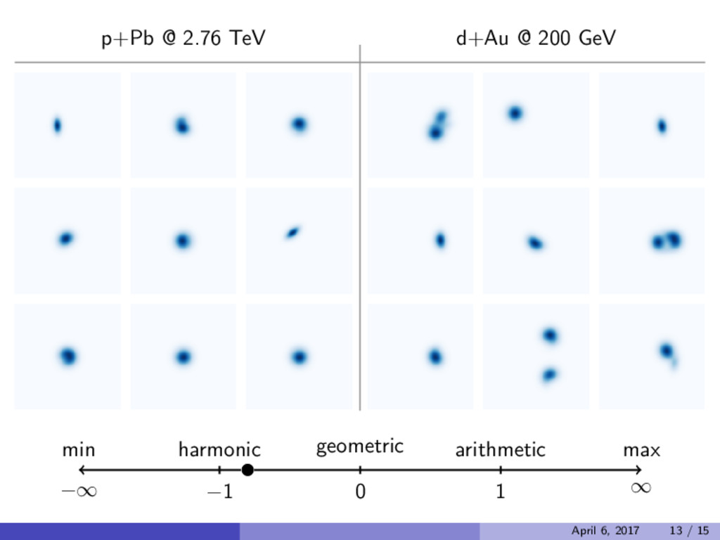
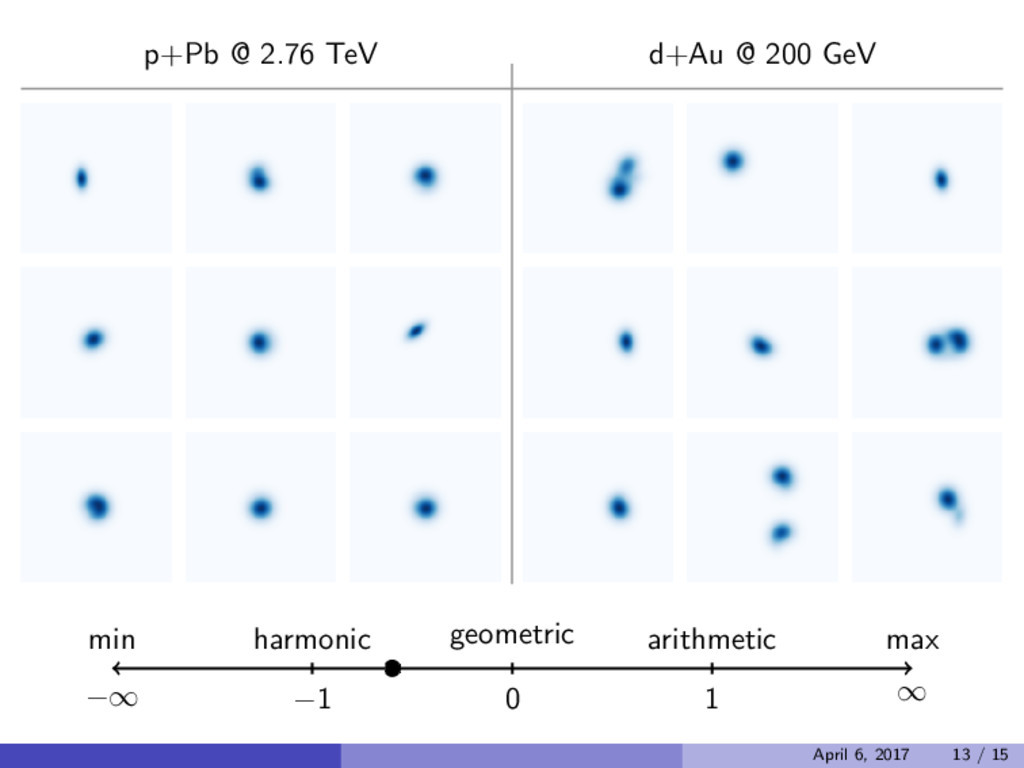
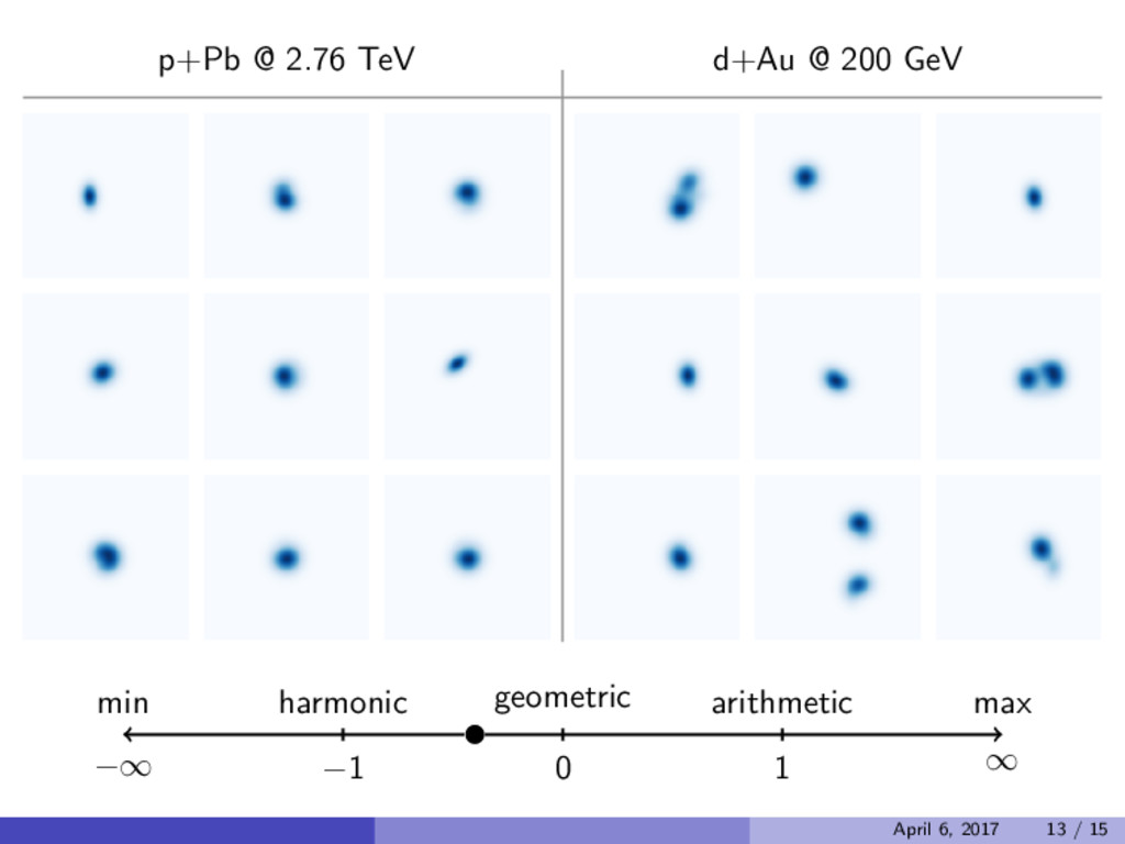
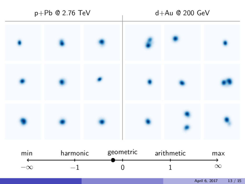
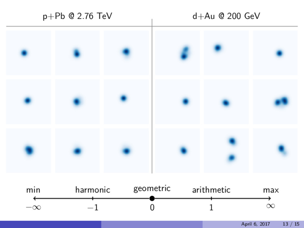
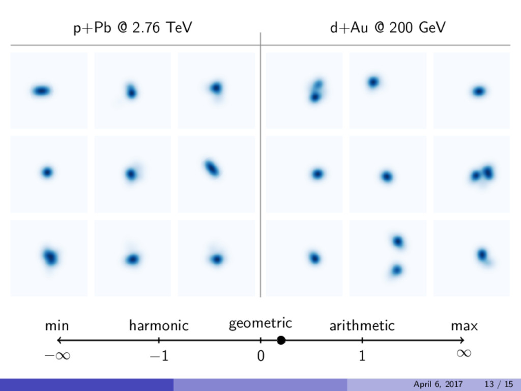
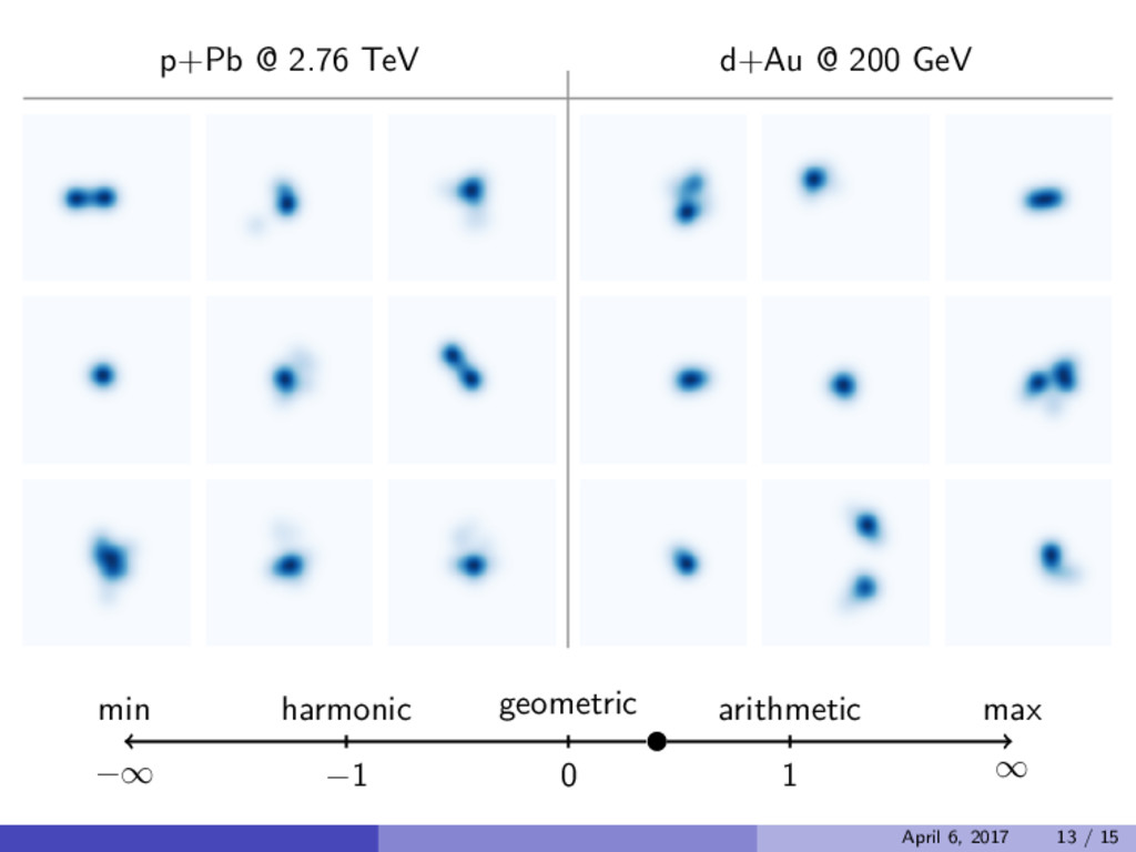
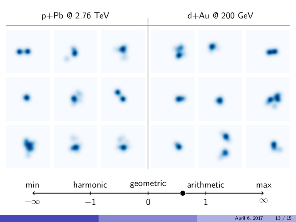
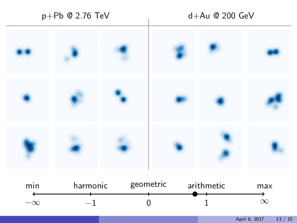
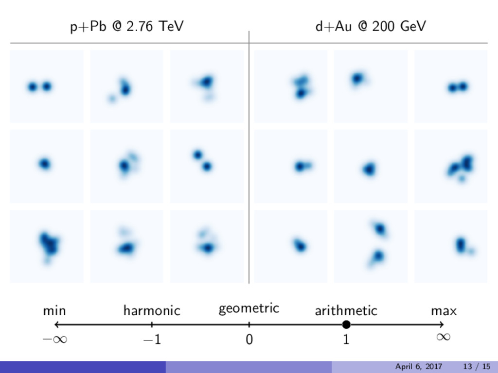
∼ TA + TB 2 Binary collision term later postulated to boost particle production in central A+A collisions dS/dy|y=0 ∼ (1 − α) TA + TB 2 + α σNNTATB In this work we replace the arithmetic mean with a generalized mean, dS/dy|y=0 ∝ Tp A + Tp B 2 1/p p = −∞ min −1 harmonic 0 geometric 1 arithmetic ∞ max April 6, 2017 4 / 15
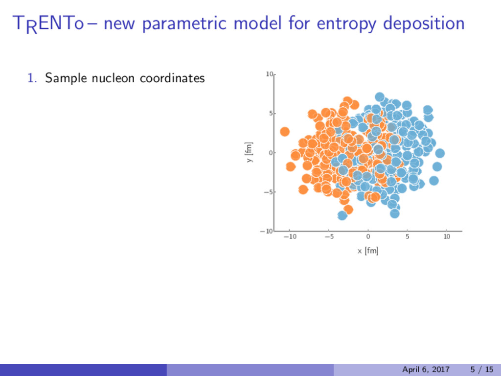
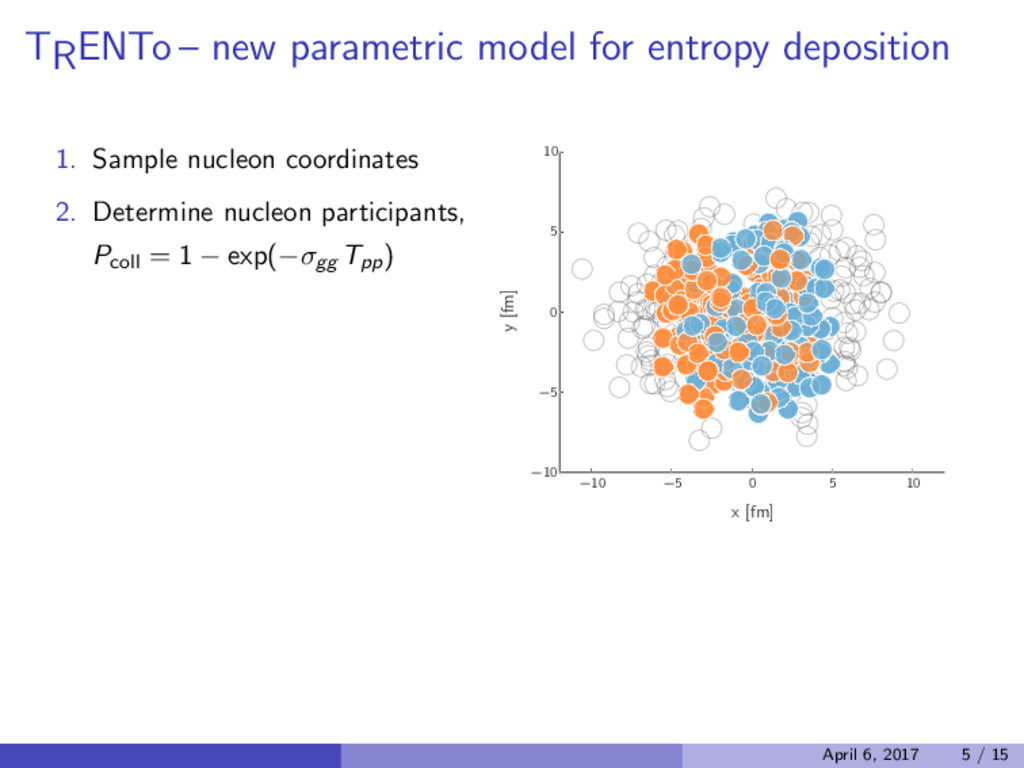
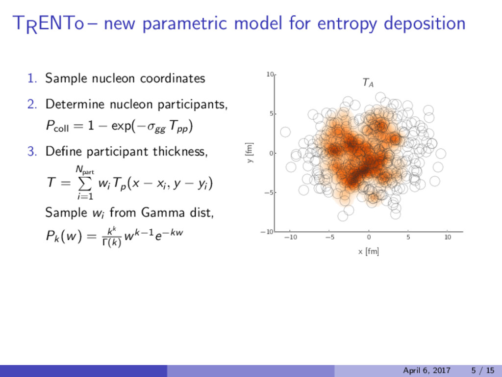
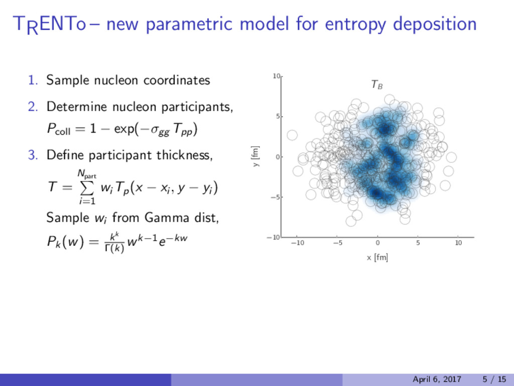
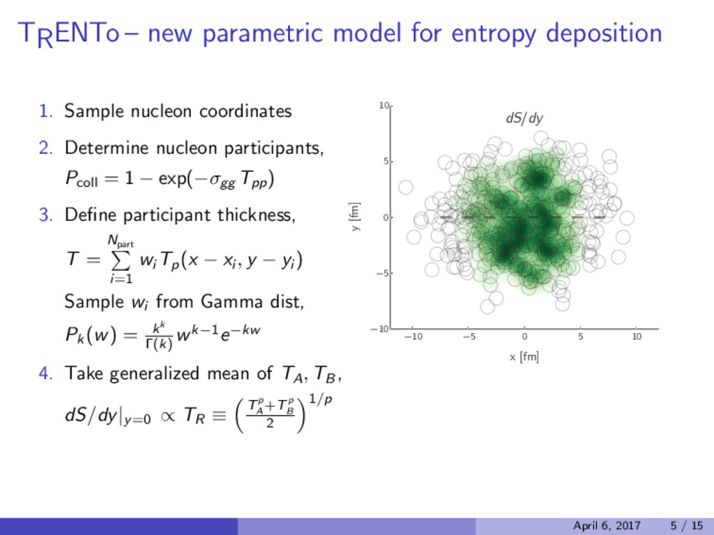
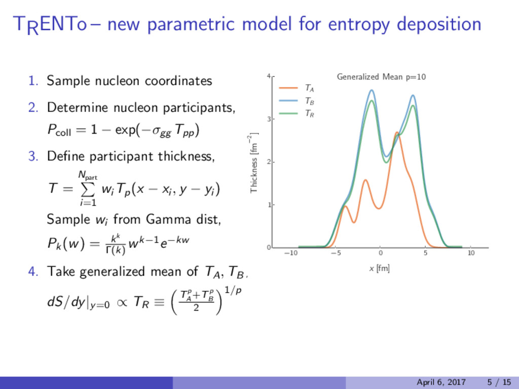
nucleon coordinates 2. Determine nucleon participants, Pcoll = 1 − exp(−σgg Tpp ) 3. Define participant thickness, T = Npart i=1 wi Tp (x − xi , y − yi ) Sample wi from Gamma dist, Pk (w) = kk Γ(k) wk−1e−kw 4. Take generalized mean of TA, TB , dS/dy|y=0 ∝ TR ≡ Tp A +Tp B 2 1/p −10 −5 0 5 10 x [fm] −10 −5 0 5 10 y [fm] dS/dy April 6, 2017 5 / 15
nucleon coordinates 2. Determine nucleon participants, Pcoll = 1 − exp(−σgg Tpp ) 3. Define participant thickness, T = Npart i=1 wi Tp (x − xi , y − yi ) Sample wi from Gamma dist, Pk (w) = kk Γ(k) wk−1e−kw 4. Take generalized mean of TA, TB , dS/dy|y=0 ∝ TR ≡ Tp A +Tp B 2 1/p −10 −5 0 5 10 x [fm] −10 −5 0 5 10 y [fm] dS/dy April 6, 2017 5 / 15
nucleon coordinates 2. Determine nucleon participants, Pcoll = 1 − exp(−σgg Tpp ) 3. Define participant thickness, T = Npart i=1 wi Tp (x − xi , y − yi ) Sample wi from Gamma dist, Pk (w) = kk Γ(k) wk−1e−kw 4. Take generalized mean of TA, TB , dS/dy|y=0 ∝ TR ≡ Tp A +Tp B 2 1/p −10 −5 0 5 10 x [fm] 0 1 2 3 4 Thickness [fm−2 ] Generalized Mean p=-10 TA TB TR April 6, 2017 5 / 15
nucleon coordinates 2. Determine nucleon participants, Pcoll = 1 − exp(−σgg Tpp ) 3. Define participant thickness, T = Npart i=1 wi Tp (x − xi , y − yi ) Sample wi from Gamma dist, Pk (w) = kk Γ(k) wk−1e−kw 4. Take generalized mean of TA, TB , dS/dy|y=0 ∝ TR ≡ Tp A +Tp B 2 1/p −10 −5 0 5 10 x [fm] 0 1 2 3 4 Thickness [fm−2 ] Generalized Mean p=1 TA TB TR April 6, 2017 5 / 15
nucleon coordinates 2. Determine nucleon participants, Pcoll = 1 − exp(−σgg Tpp ) 3. Define participant thickness, T = Npart i=1 wi Tp (x − xi , y − yi ) Sample wi from Gamma dist, Pk (w) = kk Γ(k) wk−1e−kw 4. Take generalized mean of TA, TB , dS/dy|y=0 ∝ TR ≡ Tp A +Tp B 2 1/p −10 −5 0 5 10 x [fm] 0 1 2 3 4 Thickness [fm−2 ] Generalized Mean p=10 TA TB TR April 6, 2017 5 / 15
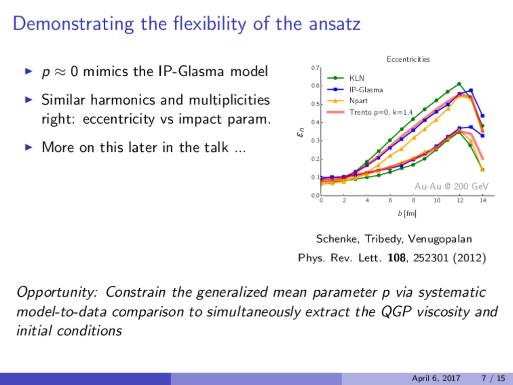
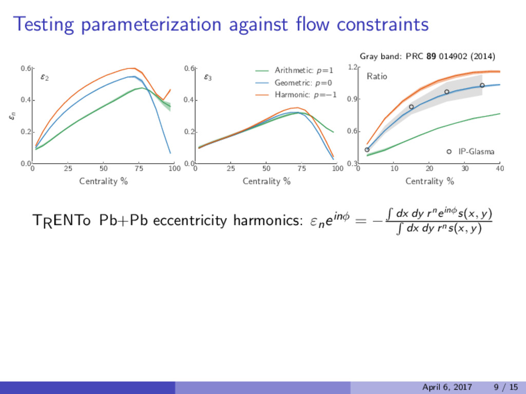
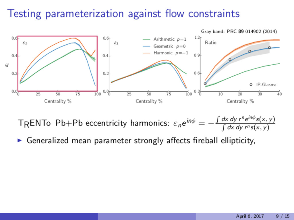
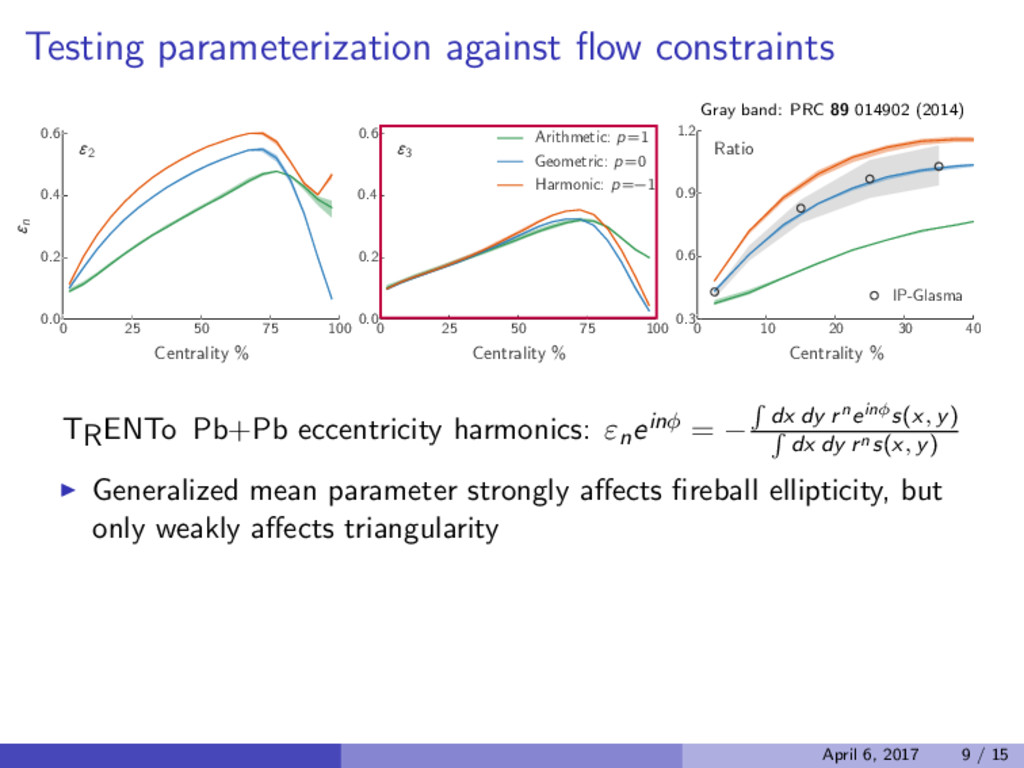
the IP-Glasma model Similar harmonics and multiplicities right: eccentricity vs impact param. More on this later in the talk ... 0 2 4 6 8 10 12 14 b [fm] 0.0 0.1 0.2 0.3 0.4 0.5 0.6 0.7 εn Au-Au @ 200 GeV Eccentricities KLN IP-Glasma Npart Trento p=0, k=1.4 Schenke, Tribedy, Venugopalan Phys. Rev. Lett. 108, 252301 (2012) Opportunity: Constrain the generalized mean parameter p via systematic model-to-data comparison to simultaneously extract the QGP viscosity and initial conditions April 6, 2017 7 / 15
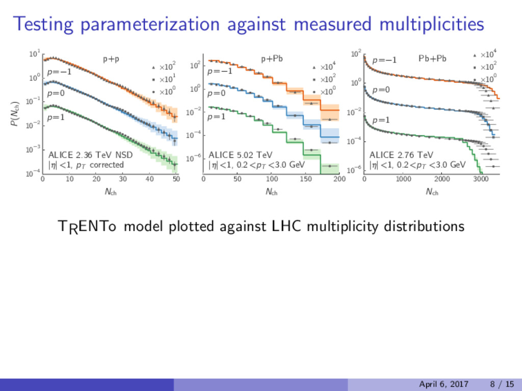
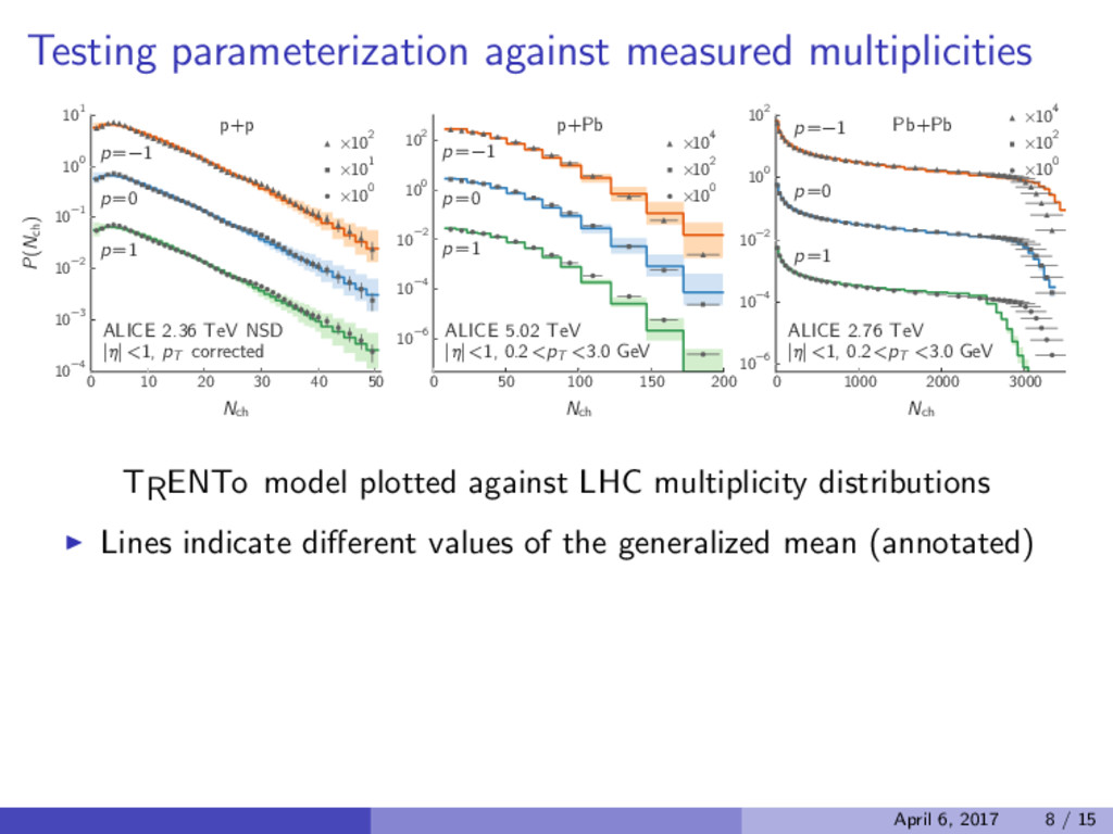
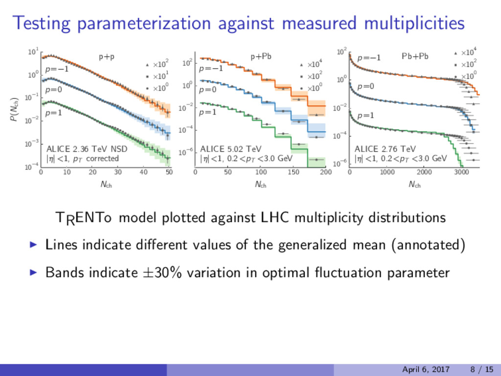
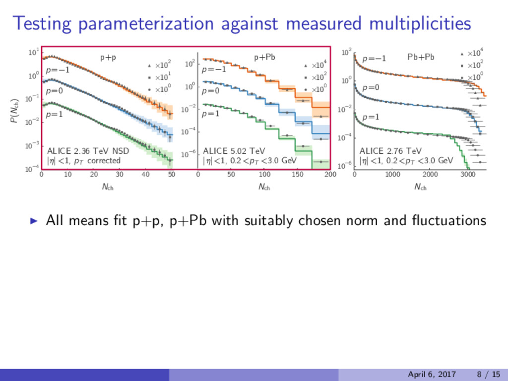
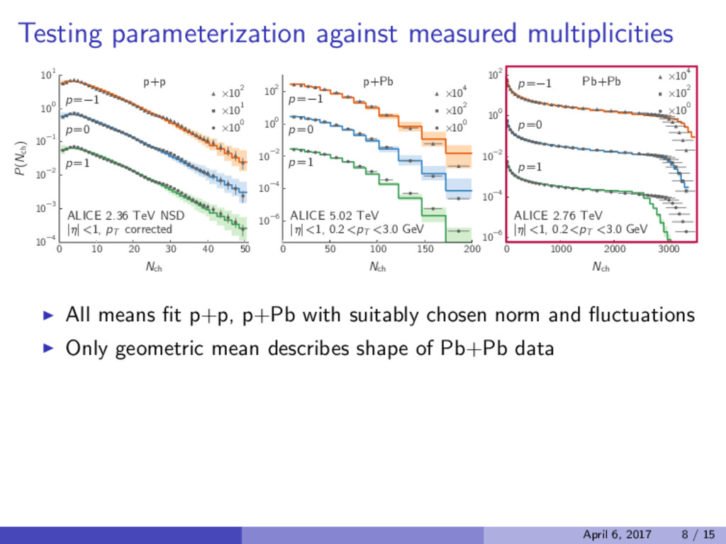
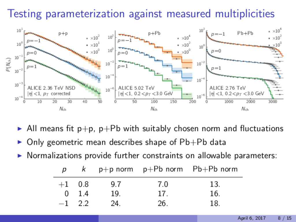
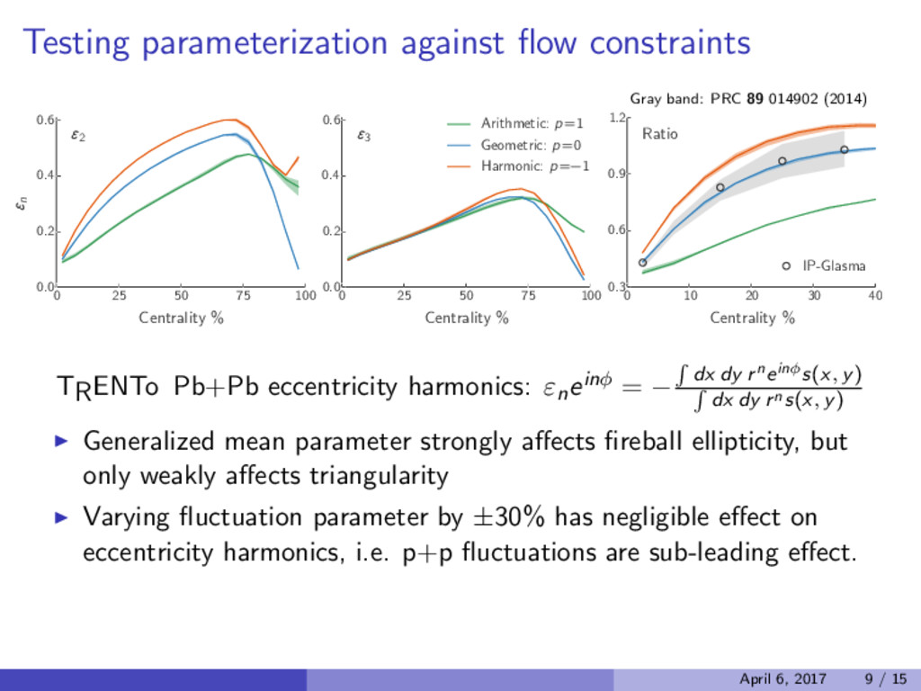
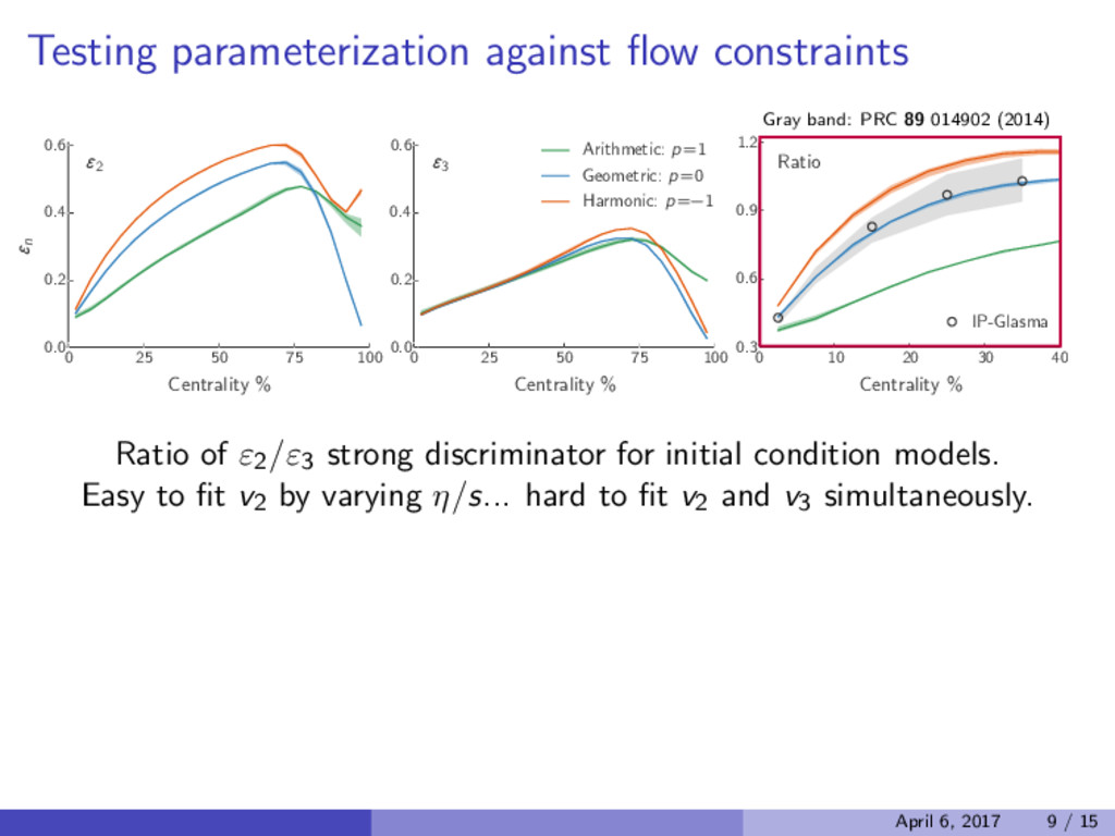
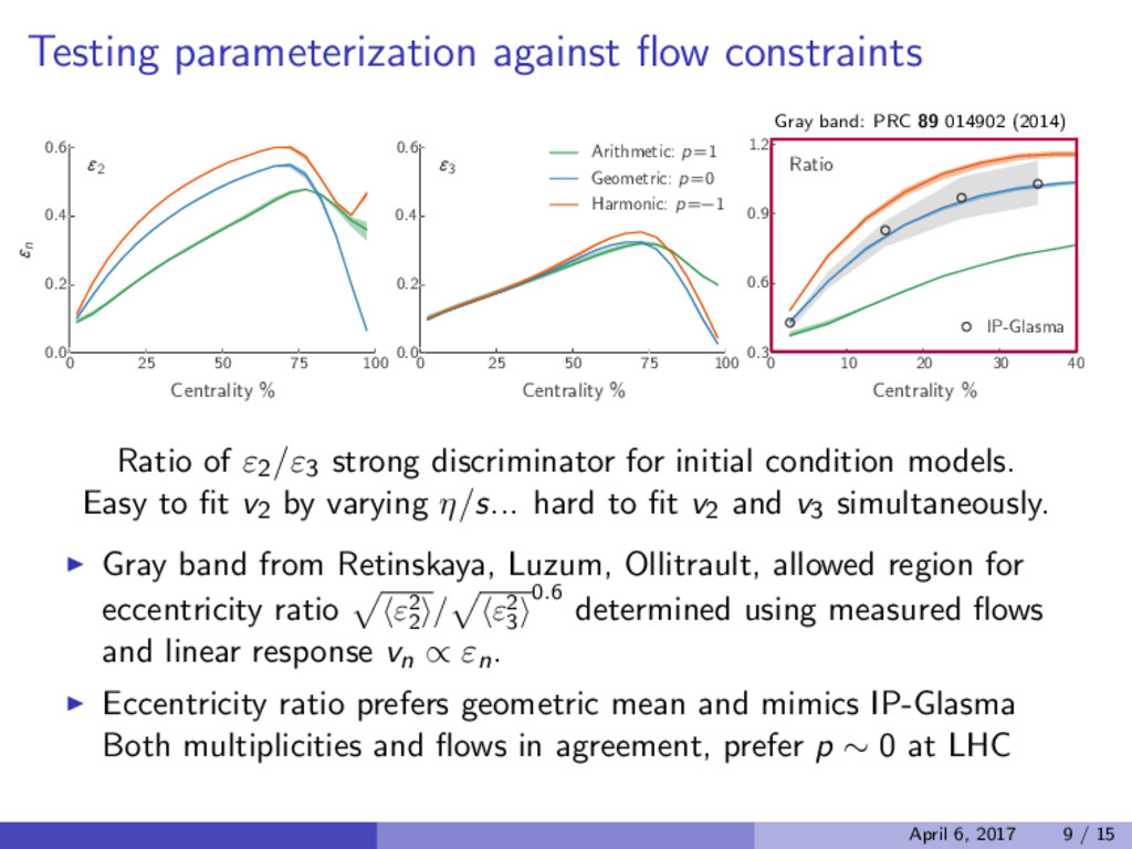
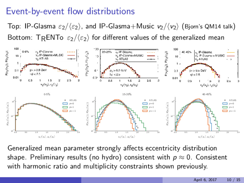
Centrality % 0.0 0.2 0.4 0.6 εn ε2 0 25 50 75 100 Centrality % 0.0 0.2 0.4 0.6 ε3 Arithmetic: p=1 Geometric: p=0 Harmonic: p=−1 0 10 20 30 40 Centrality % 0.3 0.6 0.9 1.2 Ratio IP-Glasma Gray band: PRC 89 014902 (2014) Ratio of ε2/ε3 strong discriminator for initial condition models. Easy to fit v2 by varying η/s... hard to fit v2 and v3 simultaneously. Gray band from Retinskaya, Luzum, Ollitrault, allowed region for eccentricity ratio ε2 2 / ε2 3 0.6 determined using measured flows and linear response vn ∝ εn. Eccentricity ratio prefers geometric mean and mimics IP-Glasma Both multiplicities and flows in agreement, prefer p ∼ 0 at LHC April 6, 2017 9 / 15
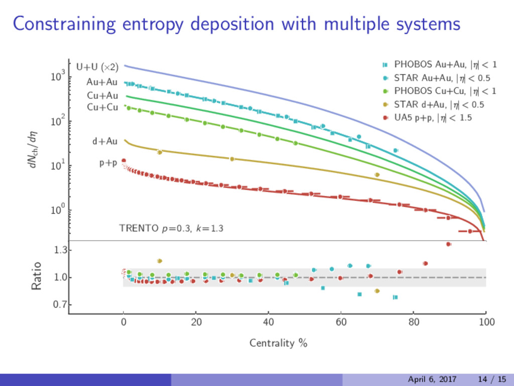
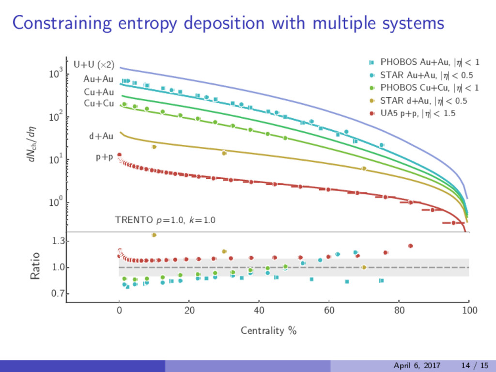
entropy proportional to the generalized mean of participant matter. Model can mimic behaviour of well known initial conditions models such as KLN and IP-Glasma. Preliminary results (no hydro!) indicate that the LHC prefers p ≈ 0 which closely mimics IP-Glasma scaling. RHIC prefers p ≈ 0.3. Model prefers entropy deposition in p+p and p+A collisions which is more eikonal, i.e. localized in p+p overlap region. Currently working on embedding model in systematic Bayesian analysis to extract QGP medium and initial state properties simultaneously. Model available at: https://github.com/Duke-QCD/trento April 6, 2017 15 / 15