uncertainty J. Scott Moreland Advisor: Steffen A. Bass SSGF Program Review Las Vegas, NV. May 25, 2016 Funding provided by DOE NNSA Stewardship Science Graduate Fellowship
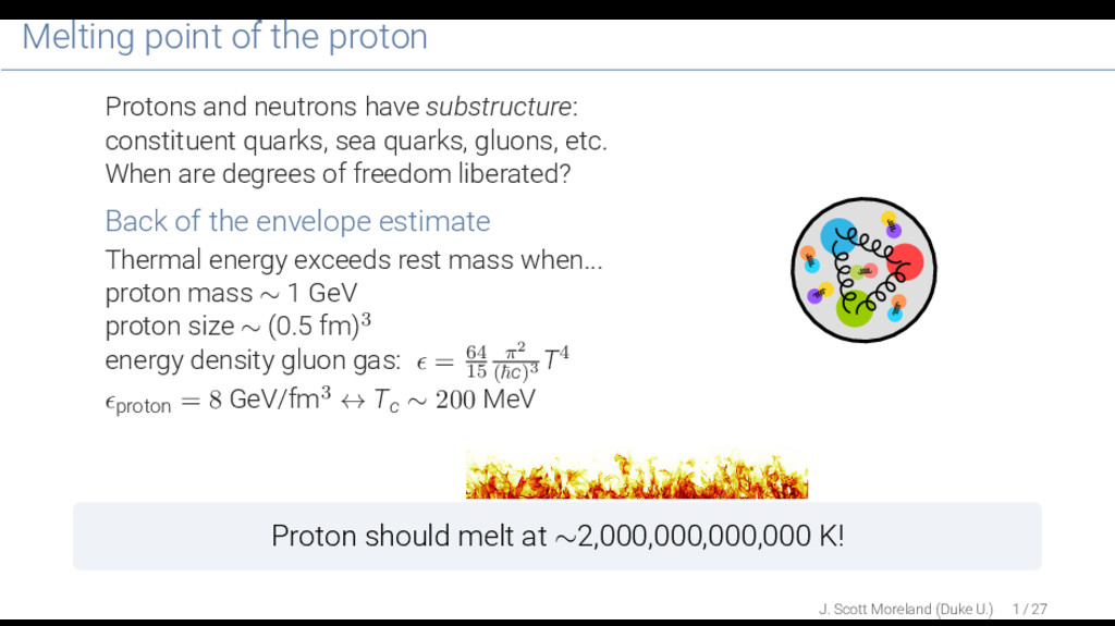
constituent quarks, sea quarks, gluons, etc. When are degrees of freedom liberated? Back of the envelope estimate Thermal energy exceeds rest mass when... proton mass ∼ 1 GeV proton size ∼ (0.5 fm)3 energy density gluon gas: = 64 15 π2 ( c)3 T4 proton = 8 GeV/fm3 ↔ Tc ∼ 200 MeV Proton should melt at ∼2,000,000,000,000 K! J. Scott Moreland (Duke U.) 1 / 27
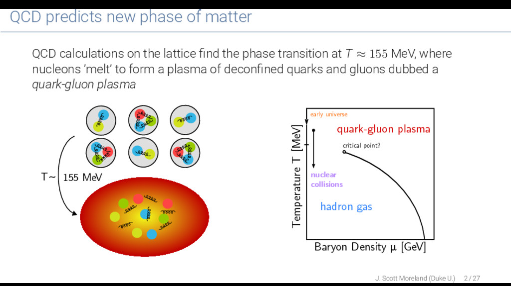
lattice find the phase transition at T ≈ 155 MeV, where nucleons ’melt’ to form a plasma of deconfined quarks and gluons dubbed a quark-gluon plasma T ~ 155 MeV Baryon Density μ [GeV] Temperature T [MeV] critical point? quark-gluon plasma early universe hadron gas nuclear collisions J. Scott Moreland (Duke U.) 2 / 27
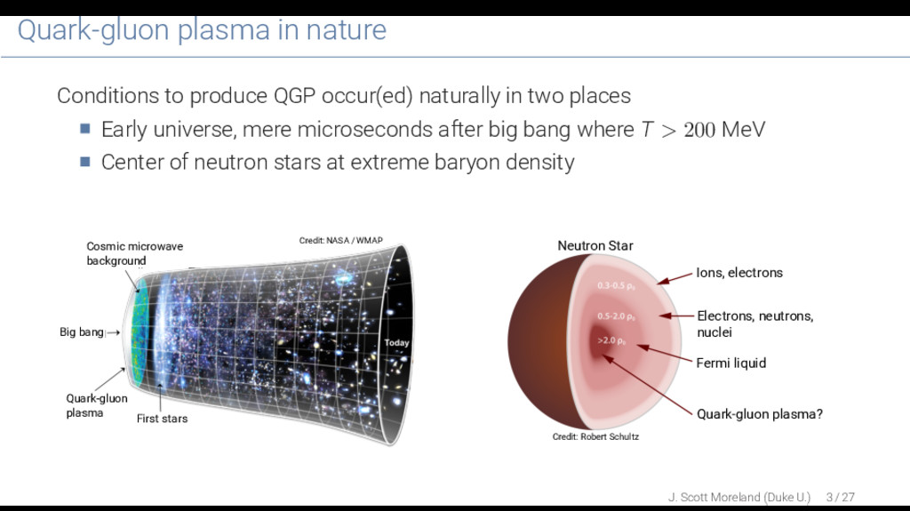
in two places Early universe, mere microseconds after big bang where T > 200 MeV Center of neutron stars at extreme baryon density Big bang First stars Quark-gluon plasma Cosmic microwave background Credit: NASA / WMAP Quark-gluon plasma? Fermi liquid Electrons, neutrons, nuclei Ions, electrons Credit: Robert Schultz Neutron Star J. Scott Moreland (Duke U.) 3 / 27
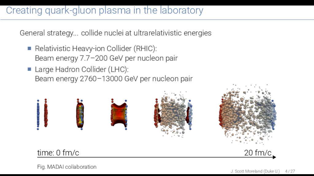
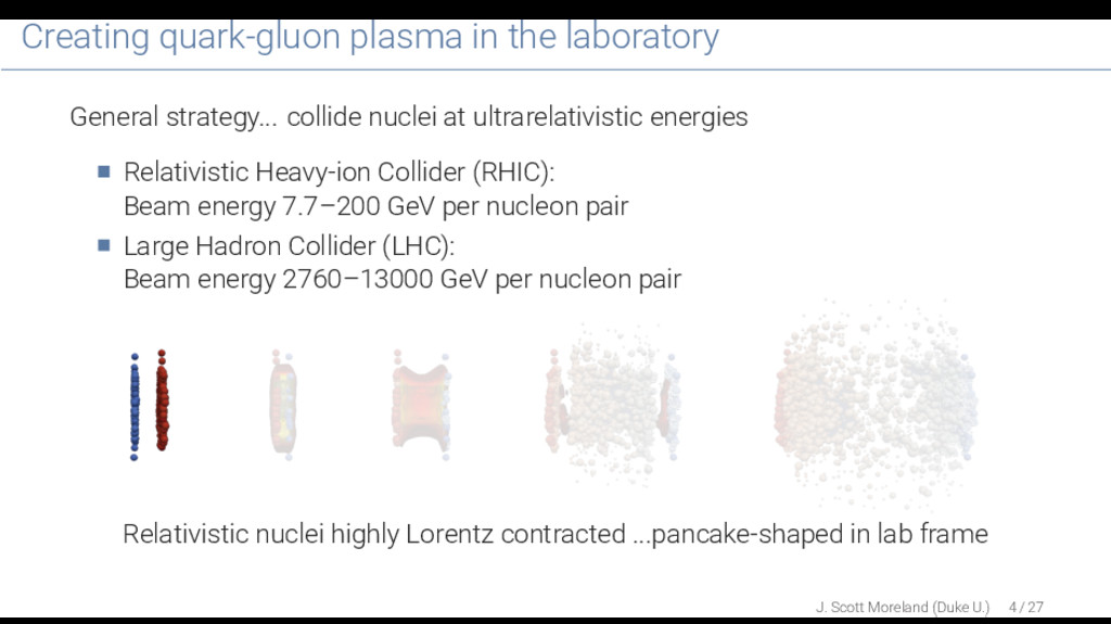
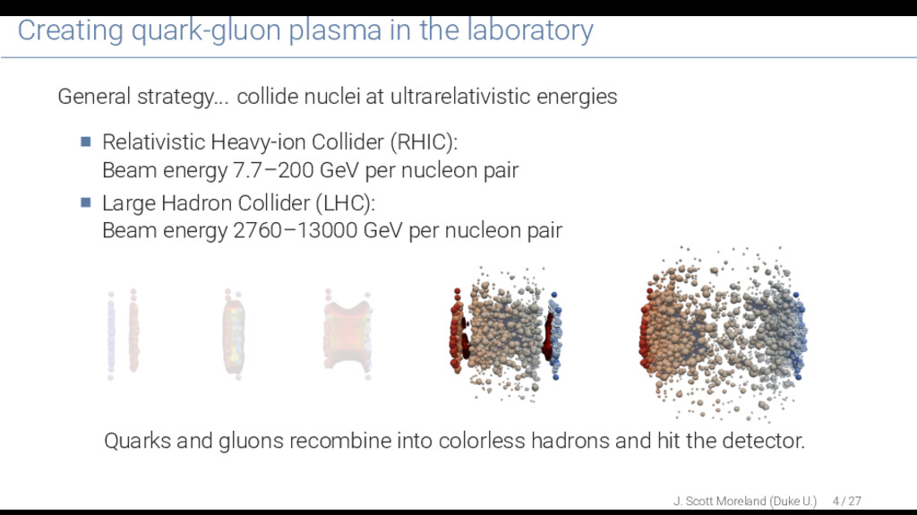
at ultrarelativistic energies Relativistic Heavy-ion Collider (RHIC): Beam energy 7.7–200 GeV per nucleon pair Large Hadron Collider (LHC): Beam energy 2760–13000 GeV per nucleon pair Relativistic nuclei highly Lorentz contracted ...pancake-shaped in lab frame J. Scott Moreland (Duke U.) 4 / 27
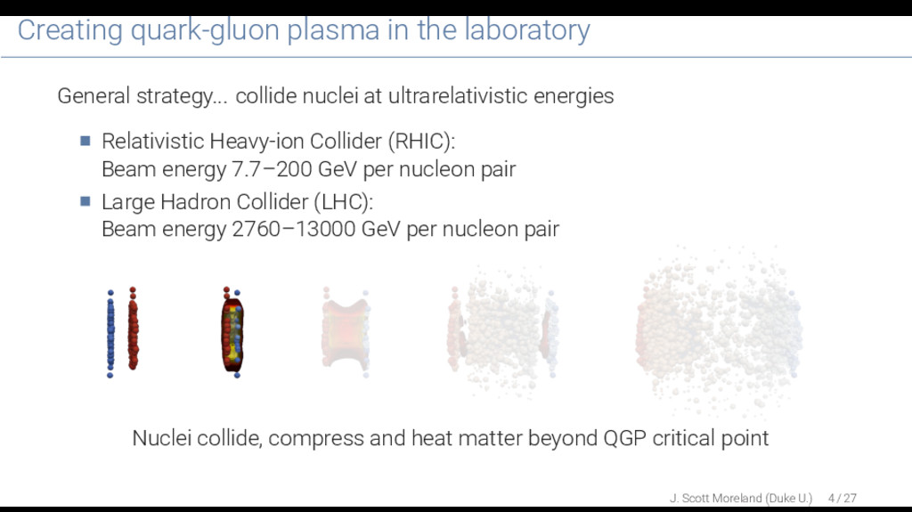
at ultrarelativistic energies Relativistic Heavy-ion Collider (RHIC): Beam energy 7.7–200 GeV per nucleon pair Large Hadron Collider (LHC): Beam energy 2760–13000 GeV per nucleon pair Nuclei collide, compress and heat matter beyond QGP critical point J. Scott Moreland (Duke U.) 4 / 27
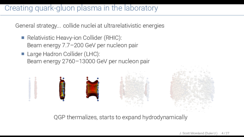
at ultrarelativistic energies Relativistic Heavy-ion Collider (RHIC): Beam energy 7.7–200 GeV per nucleon pair Large Hadron Collider (LHC): Beam energy 2760–13000 GeV per nucleon pair QGP thermalizes, starts to expand hydrodynamically J. Scott Moreland (Duke U.) 4 / 27
at ultrarelativistic energies Relativistic Heavy-ion Collider (RHIC): Beam energy 7.7–200 GeV per nucleon pair Large Hadron Collider (LHC): Beam energy 2760–13000 GeV per nucleon pair Quarks and gluons recombine into colorless hadrons and hit the detector. J. Scott Moreland (Duke U.) 4 / 27
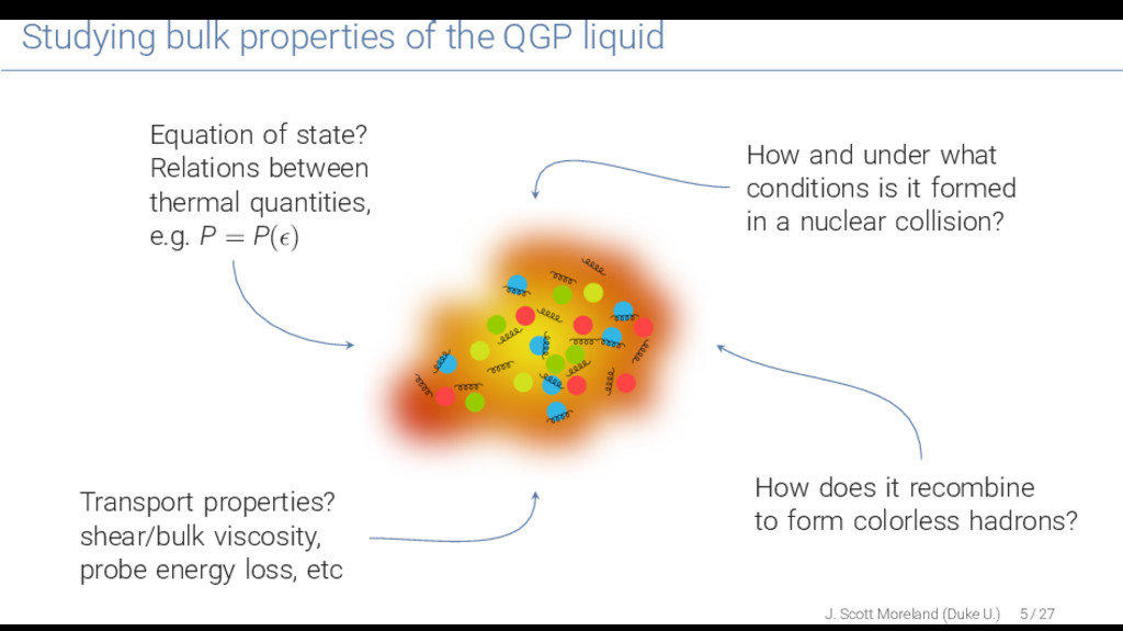
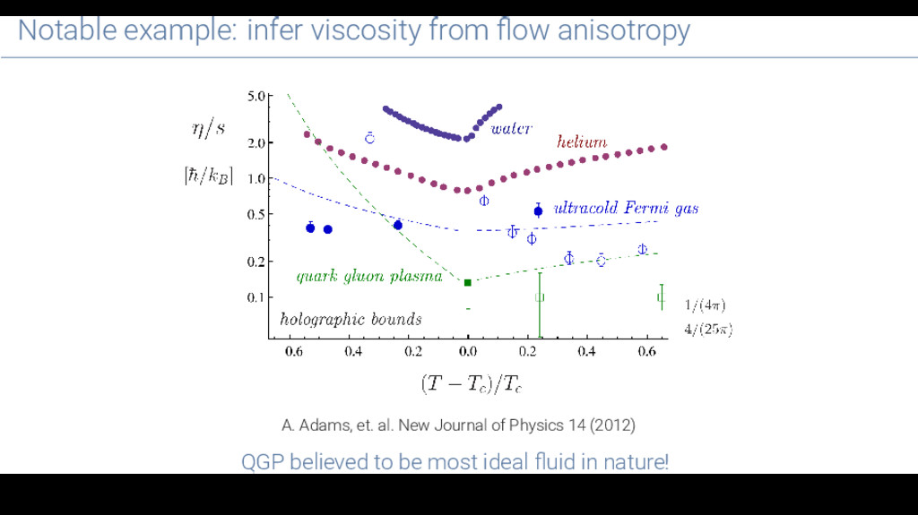
what conditions is it formed in a nuclear collision? How does it recombine to form colorless hadrons? Equation of state? Relations between thermal quantities, e.g. P = P( ) Transport properties? shear/bulk viscosity, probe energy loss, etc J. Scott Moreland (Duke U.) 5 / 27
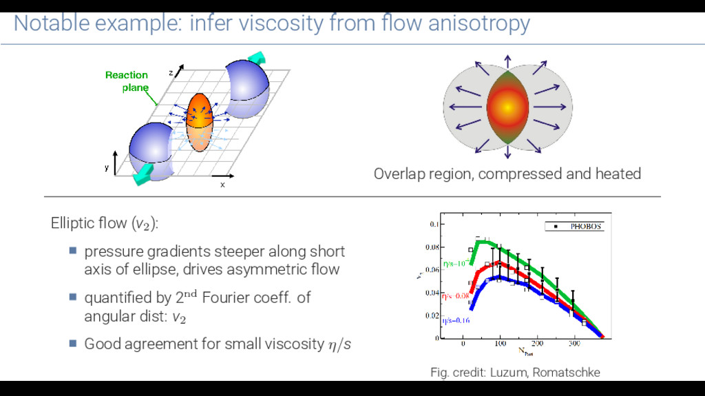
and heated Elliptic flow (v2 ): pressure gradients steeper along short axis of ellipse, drives asymmetric flow quantified by 2nd Fourier coeff. of angular dist: v2 Good agreement for small viscosity η/s Fig. credit: Luzum, Romatschke
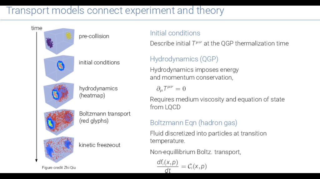
transport (red glyphs) hydrodynamics (heatmap) initial conditions pre-collision Figure credit Zhi Qiu Initial conditions Describe initial Tµν at the QGP thermalization time Hydrodynamics (QGP) Hydrodynamics imposes energy and momentum conservation, ∂µ Tµν = 0 Requires medium viscosity and equation of state from LQCD Boltzmann Eqn (hadron gas) Fluid discretized into particles at transition temperature. Non-equillibrium Boltz. transport, dfi (x, p) dt = Ci (x, p)
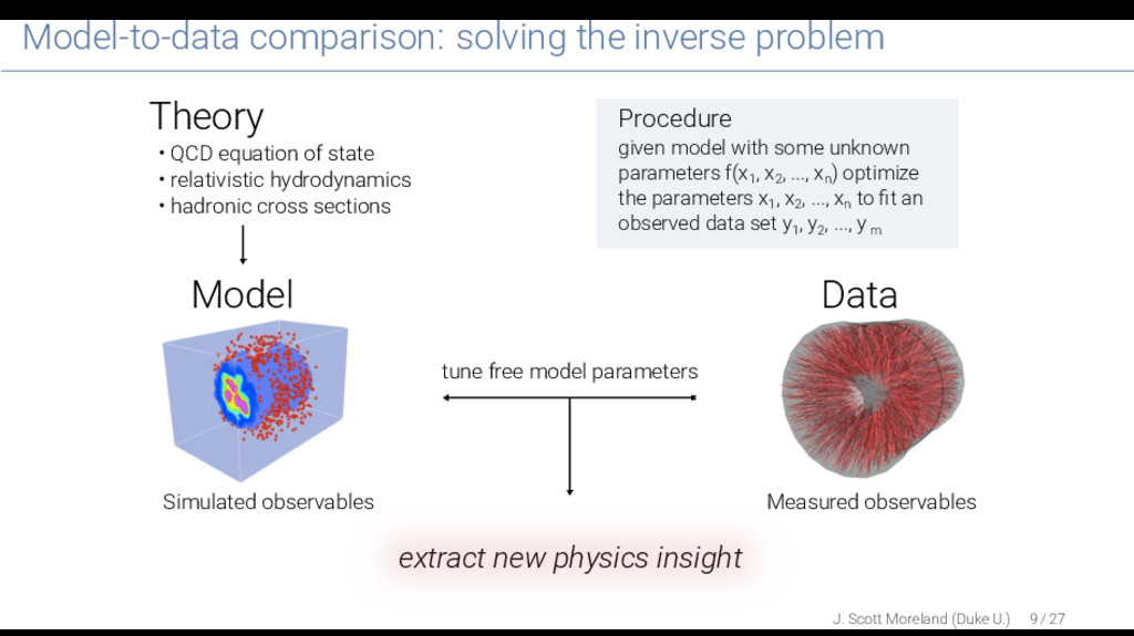
of state • relativistic hydrodynamics • hadronic cross sections Measured observables Model Data Simulated observables tune free model parameters Procedure given model with some unknown parameters f(x 1 , x 2 , ..., x n ) optimize the parameters x 1 , x 2 , ..., x n to fit an observed data set y 1 , y 2 , ..., y m extract new physics insight J. Scott Moreland (Duke U.) 9 / 27
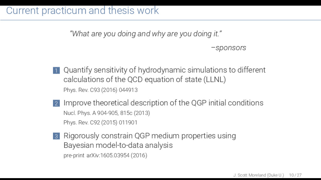
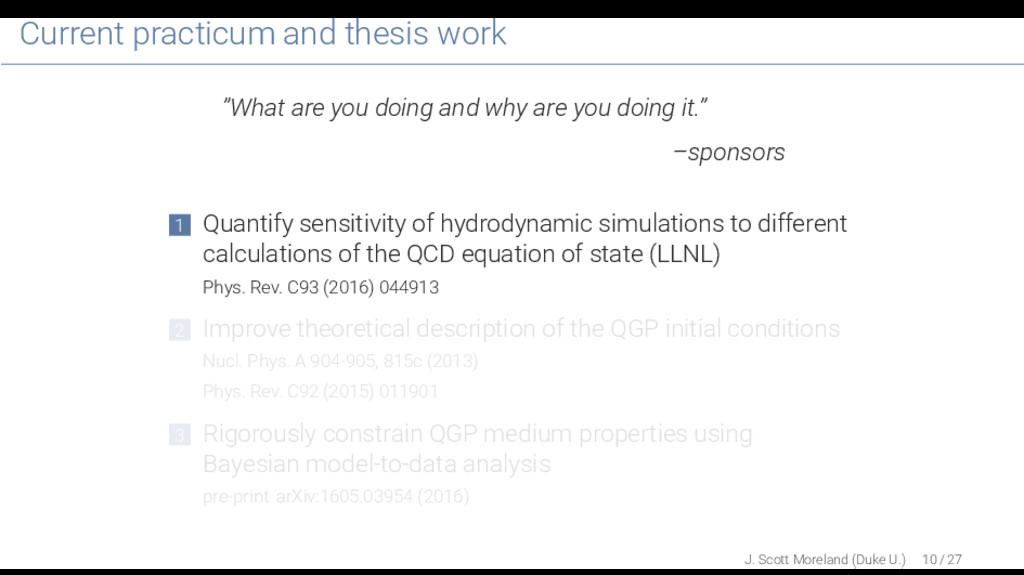
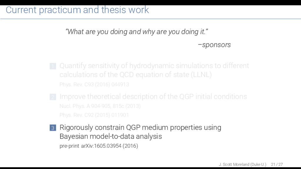
why are you doing it.” –sponsors 1 Quantify sensitivity of hydrodynamic simulations to different calculations of the QCD equation of state (LLNL) Phys. Rev. C93 (2016) 044913 2 Improve theoretical description of the QGP initial conditions Nucl. Phys. A 904-905, 815c (2013) Phys. Rev. C92 (2015) 011901 3 Rigorously constrain QGP medium properties using Bayesian model-to-data analysis pre-print arXiv:1605.03954 (2016) J. Scott Moreland (Duke U.) 10 / 27
why are you doing it.” –sponsors 1 Quantify sensitivity of hydrodynamic simulations to different calculations of the QCD equation of state (LLNL) Phys. Rev. C93 (2016) 044913 2 Improve theoretical description of the QGP initial conditions Nucl. Phys. A 904-905, 815c (2013) Phys. Rev. C92 (2015) 011901 3 Rigorously constrain QGP medium properties using Bayesian model-to-data analysis pre-print arXiv:1605.03954 (2016) J. Scott Moreland (Duke U.) 10 / 27
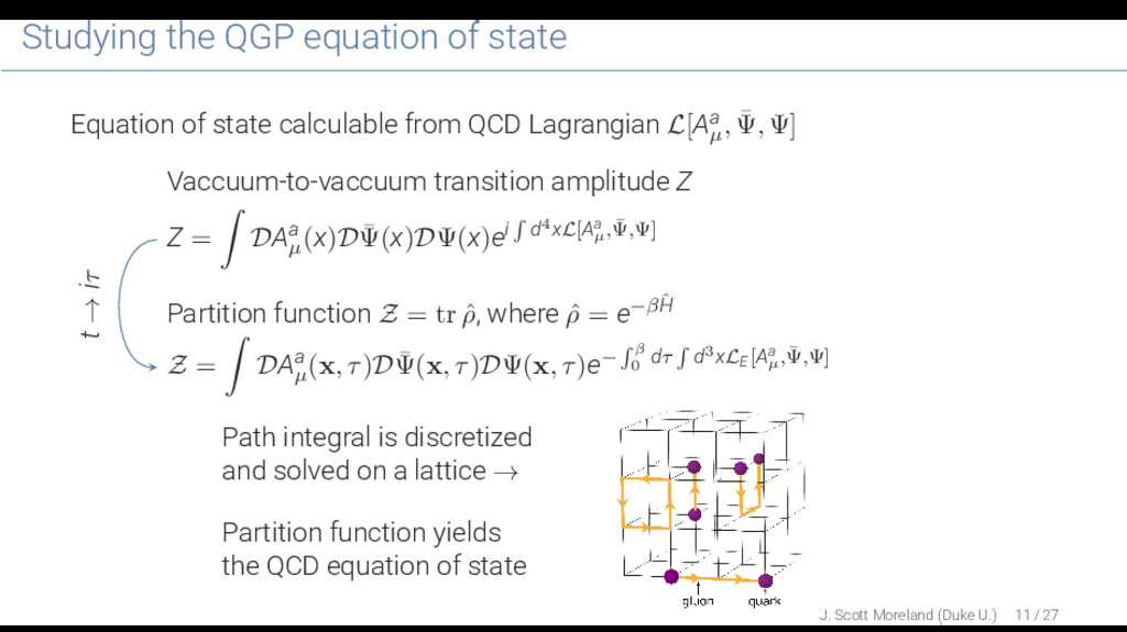
from QCD Lagrangian L[Aa µ , ¯ Ψ, Ψ] Vaccuum-to-vaccuum transition amplitude Z Z = DAa µ (x)D ¯ Ψ(x)DΨ(x)ei d4xL[Aa µ ,¯ Ψ,Ψ] Partition function Z = tr ˆ ρ, where ˆ ρ = e−βˆ H Z = DAa µ (x, τ)D ¯ Ψ(x, τ)DΨ(x, τ)e− β 0 dτ d3xLE[Aa µ ,¯ Ψ,Ψ] t → iτ Path integral is discretized and solved on a lattice → Partition function yields the QCD equation of state J. Scott Moreland (Duke U.) 11 / 27
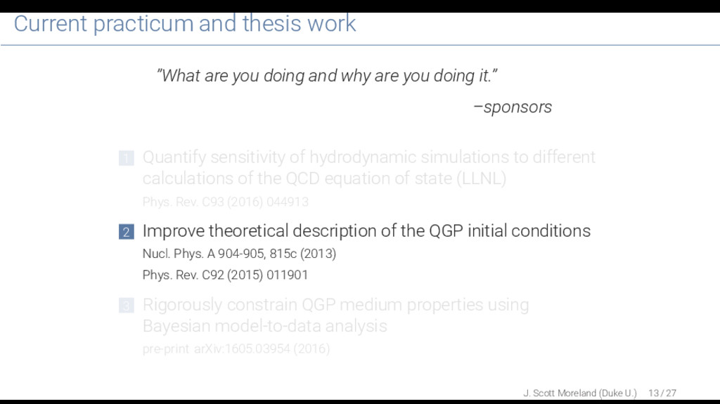
why are you doing it.” –sponsors 1 Quantify sensitivity of hydrodynamic simulations to different calculations of the QCD equation of state (LLNL) Phys. Rev. C93 (2016) 044913 2 Improve theoretical description of the QGP initial conditions Nucl. Phys. A 904-905, 815c (2013) Phys. Rev. C92 (2015) 011901 3 Rigorously constrain QGP medium properties using Bayesian model-to-data analysis pre-print arXiv:1605.03954 (2016) J. Scott Moreland (Duke U.) 13 / 27
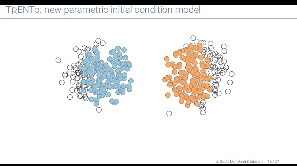
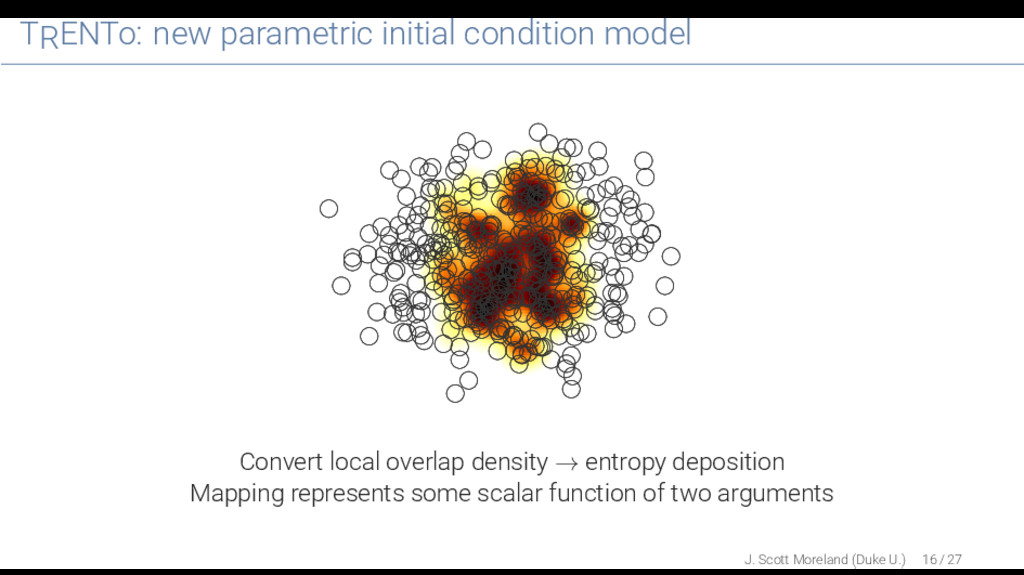
fluid velocity at τ = τ0 . Initial energy density (3D) x η x η x η Figure credit: Schenke, Schlichting Common to project out beam dimension (η-coordinate) Initial energy density (2D) −8 −4 0 4 8 x [fm] −8 −4 0 4 8 y [fm] −8 −4 0 4 8 x [fm] −8 −4 0 4 8 x [fm]
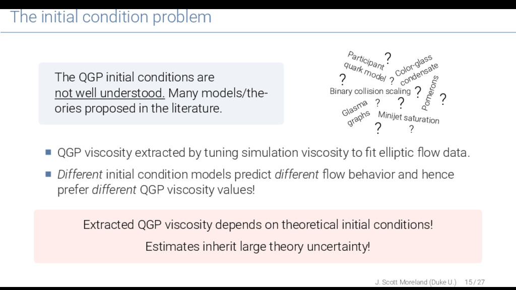
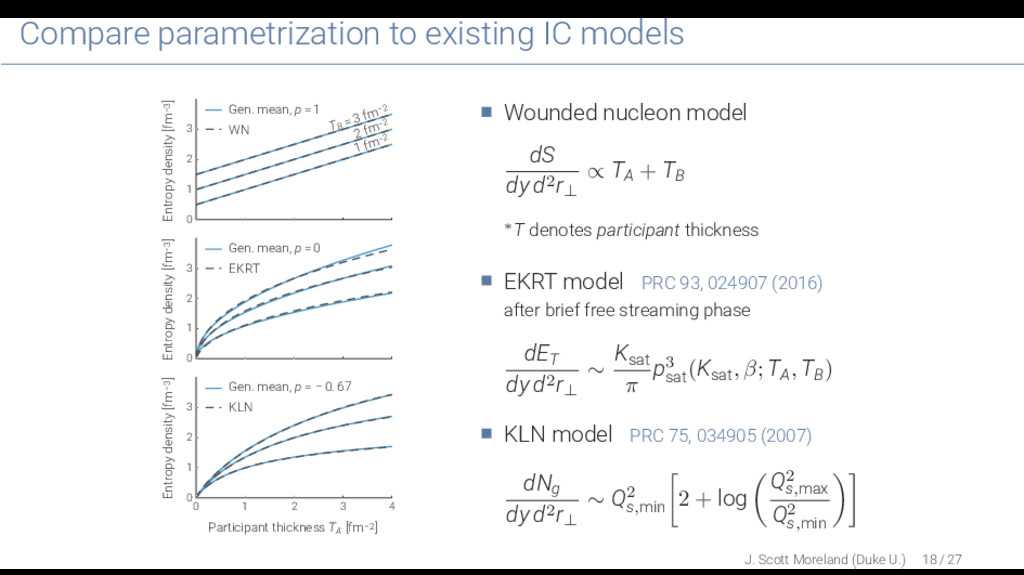
well understood. Many models/the- ories proposed in the literature. Participant quark model Glasma graphs Binary collision scaling Minijet saturation Color-glass condensate Pomerons ? ? ? ? ? ? ? ? ? QGP viscosity extracted by tuning simulation viscosity to fit elliptic flow data. Different initial condition models predict different flow behavior and hence prefer different QGP viscosity values! Extracted QGP viscosity depends on theoretical initial conditions! Estimates inherit large theory uncertainty! J. Scott Moreland (Duke U.) 15 / 27
conditions using flexible ’meta-model’. Apply rigorous statistical methods to simultaneously constrain initial condition and QGP medium parameters. J. Scott Moreland (Duke U.) 15 / 27
why are you doing it.” –sponsors 1 Quantify sensitivity of hydrodynamic simulations to different calculations of the QCD equation of state (LLNL) Phys. Rev. C93 (2016) 044913 2 Improve theoretical description of the QGP initial conditions Nucl. Phys. A 904-905, 815c (2013) Phys. Rev. C92 (2015) 011901 3 Rigorously constrain QGP medium properties using Bayesian model-to-data analysis pre-print arXiv:1605.03954 (2016) J. Scott Moreland (Duke U.) 21 / 27
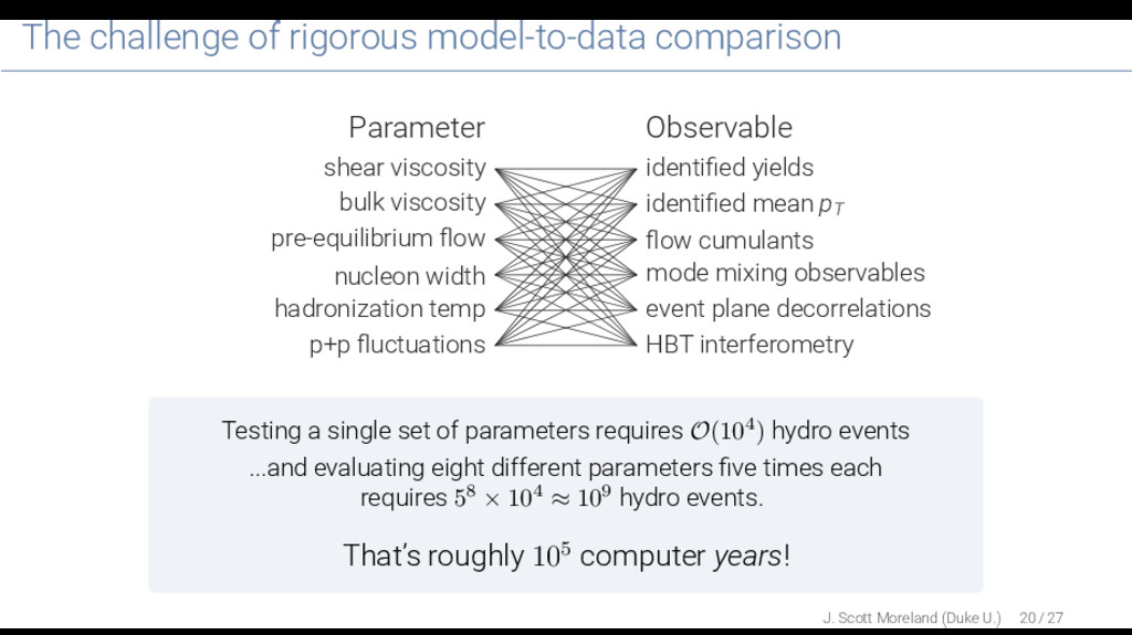
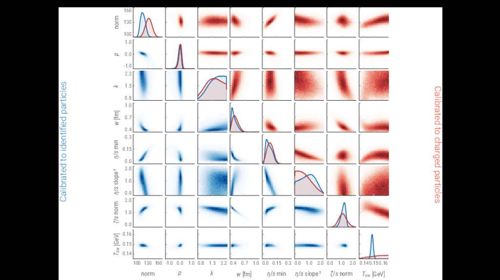
conditions (e.g. nucleon width) • QGP & HRG medium (e.g. η/s) Physics Model • TRENTo IC • iEBE-VISHNU Experimental Data • ALICE flow and spectra Gaussian Process Emulator • non-parameteric interpolation • fast surrogate for full model Markov chain Monte Carlo (MCMC) • random walk through param. space weighted by posterior probability Bayes' Theorem: posterior ∝ likelihood × posterior Posterior Distribution • probability distribution for true values of model parameters after many steps, MCMC equilibriates to calc events on Latin hypercube J. Scott Moreland (Duke U.) 22 / 27
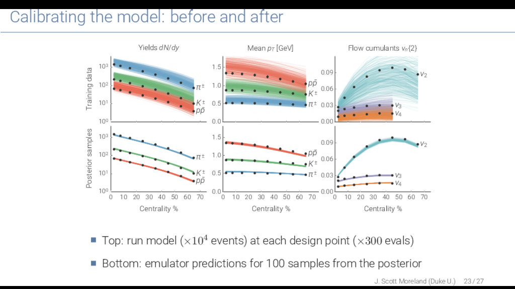
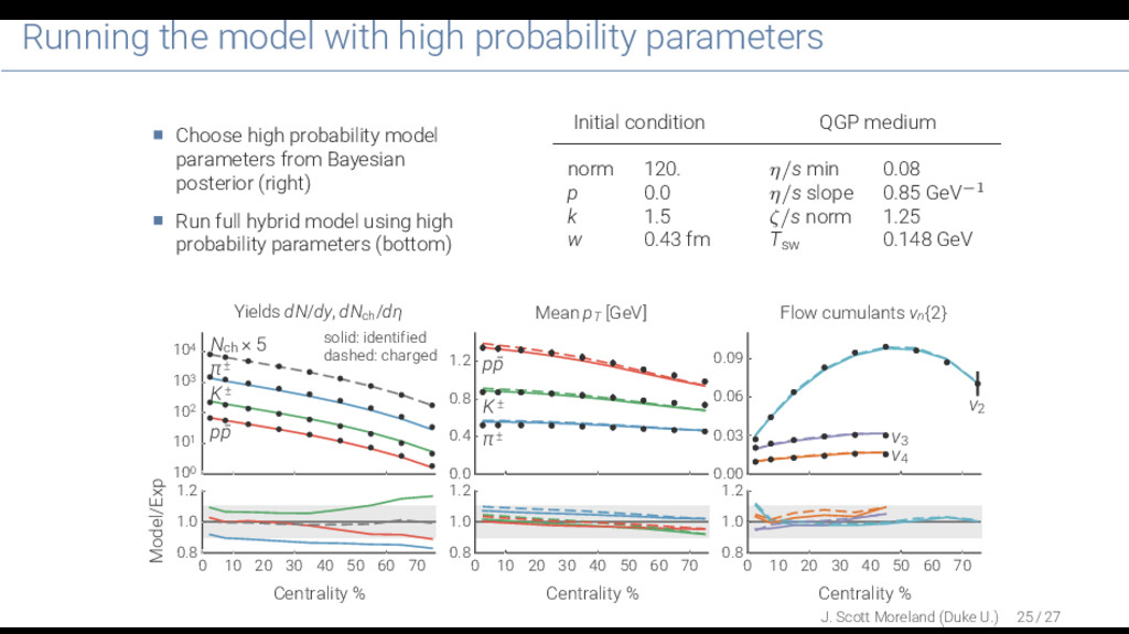
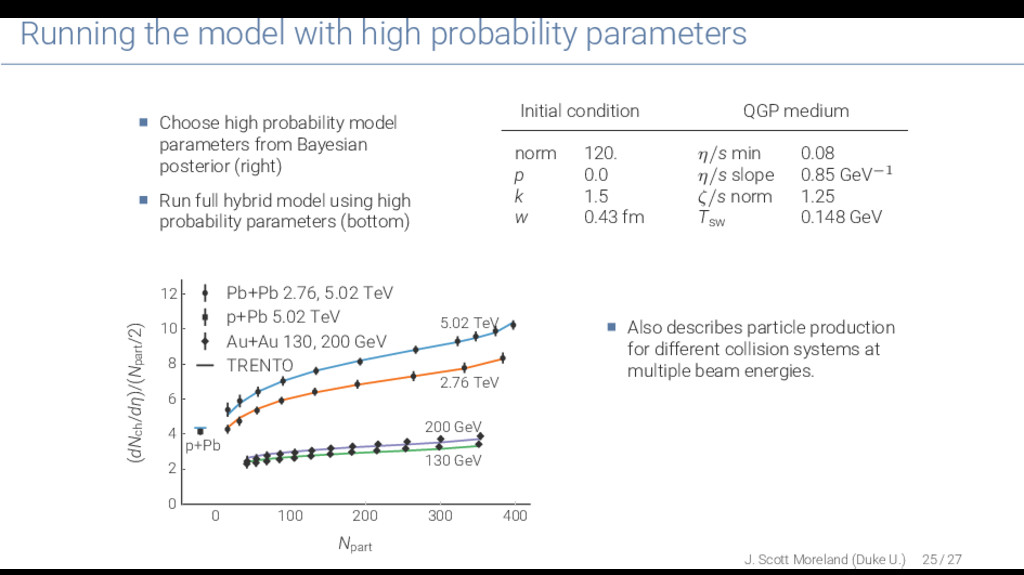
model parameters from Bayesian posterior (right) Run full hybrid model using high probability parameters (bottom) Initial condition QGP medium norm 120. η/s min 0.08 p 0.0 η/s slope 0.85 GeV−1 k 1.5 ζ/s norm 1.25 w 0.43 fm Tsw 0.148 GeV 0 100 200 300 400 Npart 0 2 4 6 8 10 12 (dNch /dη)/(Npart /2) p+Pb 5.02 TeV 2.76 TeV 200 GeV 130 GeV Pb+Pb 2.76, 5.02 TeV p+Pb 5.02 TeV Au+Au 130, 200 GeV TRENTO Also describes particle production for different collision systems at multiple beam energies. J. Scott Moreland (Duke U.) 25 / 27
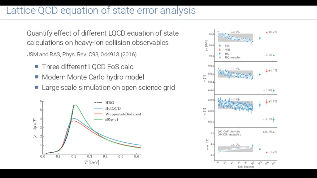
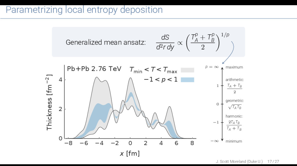
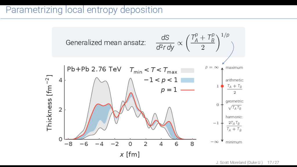
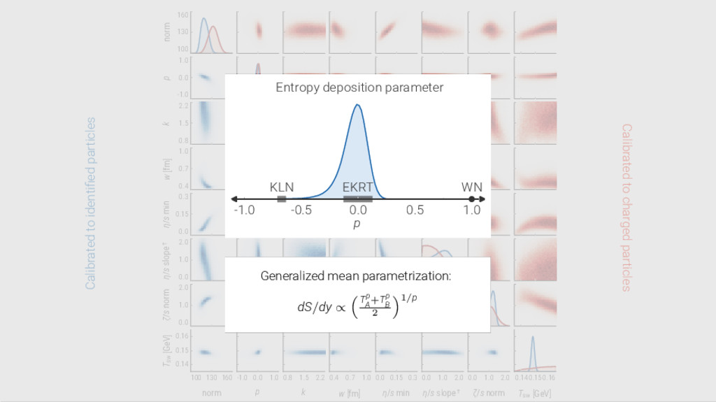
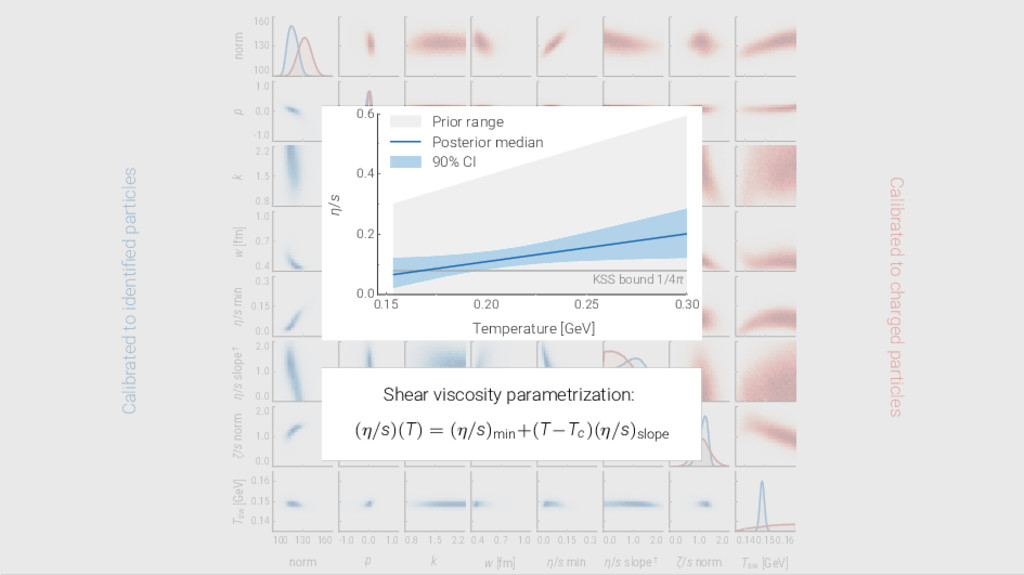
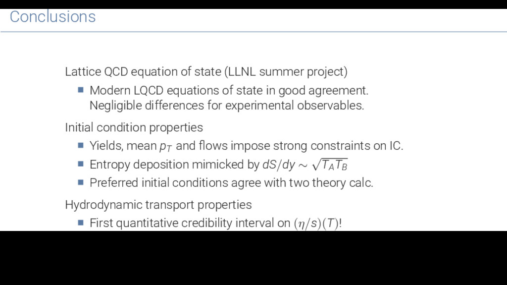
LQCD equations of state in good agreement. Negligible differences for experimental observables. Initial condition properties Yields, mean pT and flows impose strong constraints on IC. Entropy deposition mimicked by dS/dy ∼ √ TA TB Preferred initial conditions agree with two theory calc. Hydrodynamic transport properties First quantitative credibility interval on (η/s)(T)!
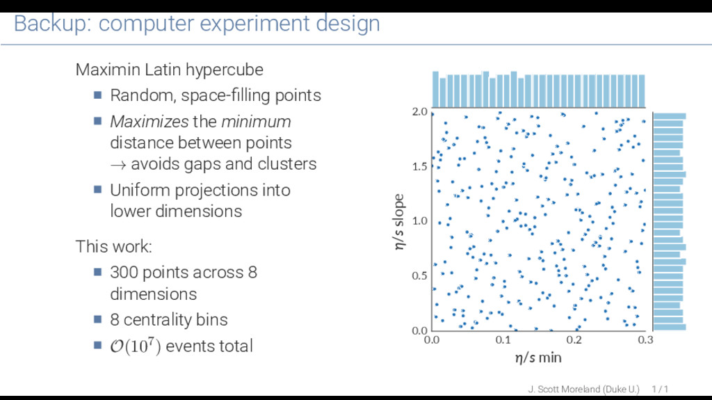
Maximizes the minimum distance between points → avoids gaps and clusters Uniform projections into lower dimensions This work: 300 points across 8 dimensions 8 centrality bins O(107) events total 0.0 0.1 0.2 0.3 η/s min 0.0 0.5 1.0 1.5 2.0 η/s slope J. Scott Moreland (Duke U.) 1 / 1