Determining QGP initial conditions and medium properties via Bayesian model-to-data analysis

Initial Stages International Conference on High Energy Nuclear Collisions, Lisbon, Portugal

Transcript

1. Determining QGP initial conditions and medium properties via Bayesian model-to-data analysis J.S. Moreland, J.E. Bernhard, S.A. Bass J. Liu, U. Heinz arXiv:1605.03954 Initial Stages | May 25, 2016 Funding provided by DOE Stewardship Science Graduate Fellowship
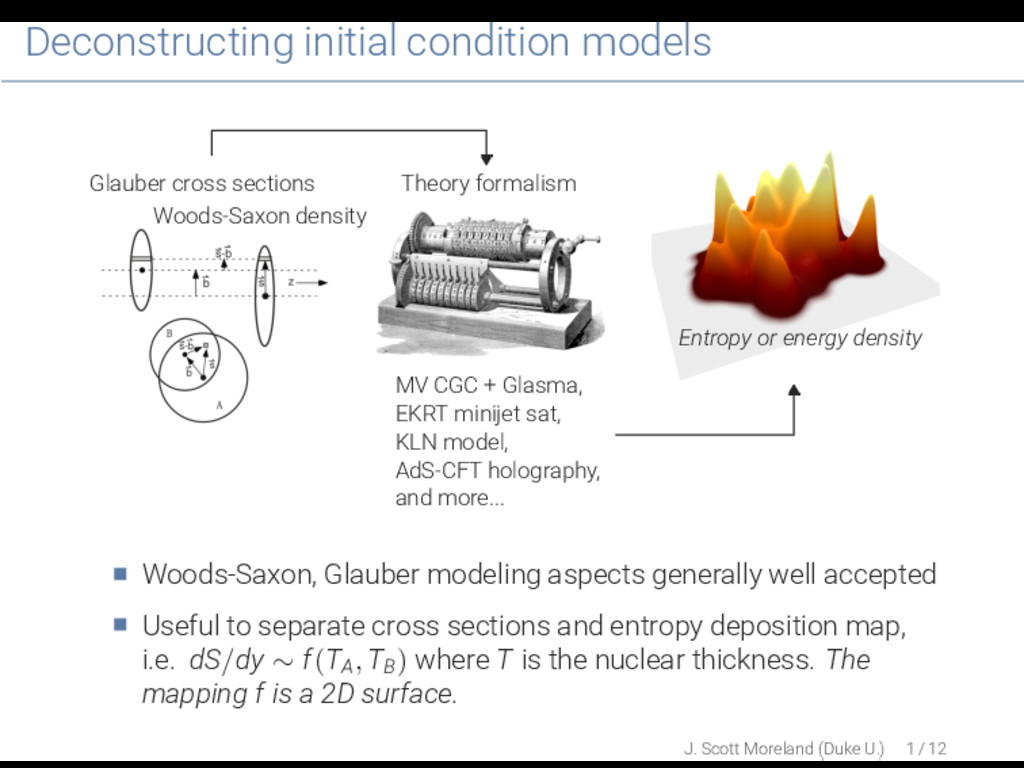
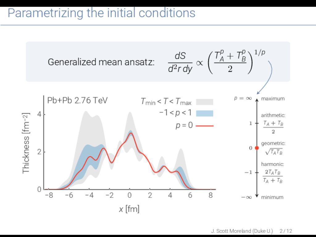
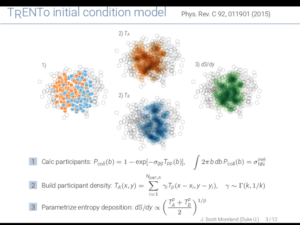
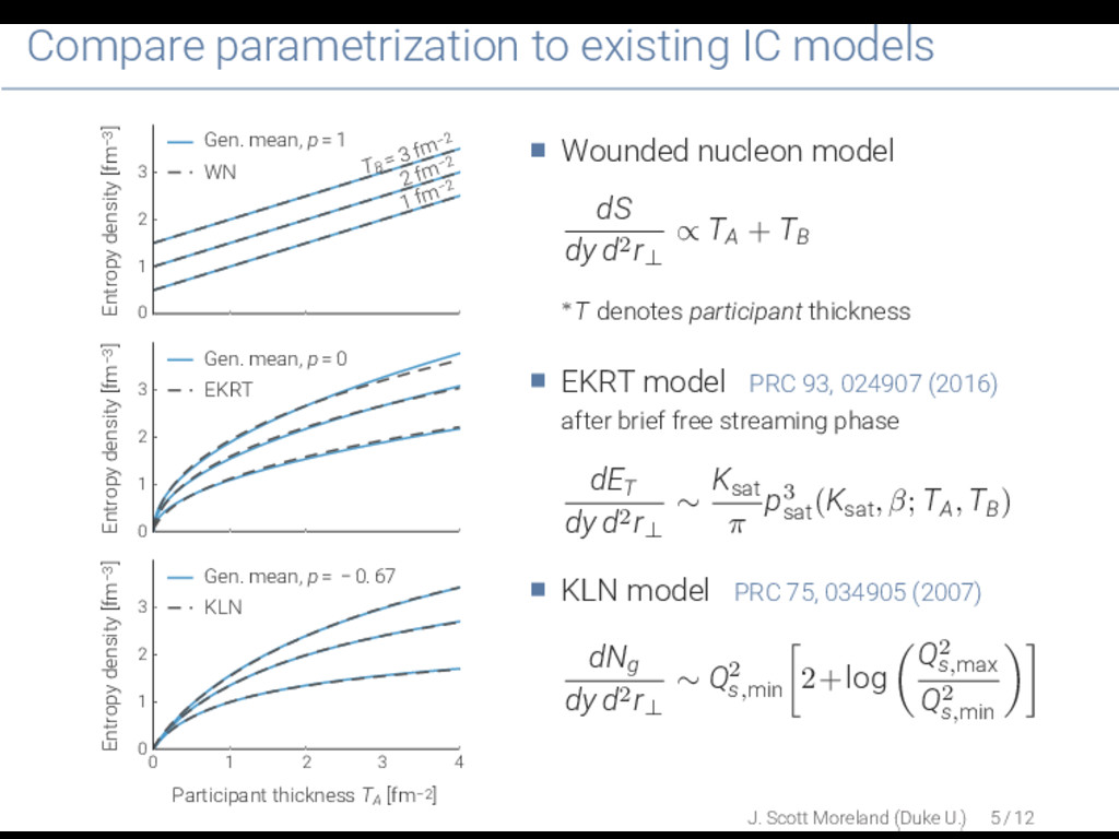
2. Deconstructing initial condition models MV CGC + Glasma, EKRT minijet sat, KLN model, AdS-CFT holography, and more... Glauber cross sections Woods-Saxon density Entropy or energy density Theory formalism Woods-Saxon, Glauber modeling aspects generally well accepted Useful to separate cross sections and entropy deposition map, i.e. dS/dy ∼ f(TA, TB) where T is the nuclear thickness. The mapping f is a 2D surface. J. Scott Moreland (Duke U.) 1 / 12
3. Parametrizing the initial conditions Generalized mean ansatz: dS d2r dy ∝ Tp A + Tp B 2 1/p −8 −6 −4 −2 0 2 4 6 8 x [fm] 0 2 4 Thickness [fm−2] Pb+Pb 2.76 TeV Tmin < T < Tmax −1 < p < 1 p = ∞ maximum 1 arithmetic: TA + TB 2 0 geometric: TATB −1 harmonic: 2TATB TA + TB −∞ minimum J. Scott Moreland (Duke U.) 2 / 12
4. Parametrizing the initial conditions Generalized mean ansatz: dS d2r dy ∝ Tp A + Tp B 2 1/p −8 −6 −4 −2 0 2 4 6 8 x [fm] 0 2 4 Thickness [fm−2] Pb+Pb 2.76 TeV Tmin < T < Tmax −1 < p < 1 p = 1 p = ∞ maximum 1 arithmetic: TA + TB 2 0 geometric: TATB −1 harmonic: 2TATB TA + TB −∞ minimum J. Scott Moreland (Duke U.) 2 / 12
5. Parametrizing the initial conditions Generalized mean ansatz: dS d2r dy ∝ Tp A + Tp B 2 1/p −8 −6 −4 −2 0 2 4 6 8 x [fm] 0 2 4 Thickness [fm−2] Pb+Pb 2.76 TeV Tmin < T < Tmax −1 < p < 1 p = 0 p = ∞ maximum 1 arithmetic: TA + TB 2 0 geometric: TATB −1 harmonic: 2TATB TA + TB −∞ minimum J. Scott Moreland (Duke U.) 2 / 12
6. Parametrizing the initial conditions Generalized mean ansatz: dS d2r dy ∝ Tp A + Tp B 2 1/p −8 −6 −4 −2 0 2 4 6 8 x [fm] 0 2 4 Thickness [fm−2] Pb+Pb 2.76 TeV Tmin < T < Tmax −1 < p < 1 p = − 1 p = ∞ maximum 1 arithmetic: TA + TB 2 0 geometric: TATB −1 harmonic: 2TATB TA + TB −∞ minimum J. Scott Moreland (Duke U.) 2 / 12
7. TRENTo initial condition model Phys. Rev. C 92, 011901 (2015) 1) 2) TA 2) TB 3) dS/dy 1 Calc participants: Pcoll(b) = 1 − exp[−σggTpp(b)], 2π b db Pcoll(b) = σinel NN 2 Build participant density: TA(x, y) = Npart,A i=1 γiTp(x − xi, y − yi), γ ∼ Γ(k, 1/k) 3 Parametrize entropy deposition: dS/dy ∝ Tp A + Tp B 2 1/p J. Scott Moreland (Duke U.) 3 / 12
9. Compare parametrization to existing IC models 0 1 2 3 Entropy density [fm−3] 1 fm−2 2 fm−2 TB = 3 fm−2 Gen. mean, p = 1 WN 0 1 2 3 Entropy density [fm−3] Gen. mean, p = 0 EKRT 0 1 2 3 4 Participant thickness TA [fm−2] 0 1 2 3 Entropy density [fm−3] Gen. mean, p = − 0. 67 KLN Wounded nucleon model dS dy d2r⊥ ∝ TA + TB ∗T denotes participant thickness EKRT model PRC 93, 024907 (2016) after brief free streaming phase dET dy d2r⊥ ∼ Ksat π p3 sat (Ksat, β; TA, TB) KLN model PRC 75, 034905 (2007) dNg dy d2r⊥ ∼ Q2 s,min 2+log Q2 s,max Q2 s,min J. Scott Moreland (Duke U.) 5 / 12
10. Modern event-by-event hybrid model TRENTo initial conditions Moreland, Bernhard, Bass, PRC 92, no. 1, 011901 (2015) norm entropy normalization p entropy deposition parameter k proton-proton multiplicity fluctuations w Gaussian nucleon width HotQCD equation of state Bazavov, et. al. PRD 90, 094503 (2014) iEBE-VISHNU hydrodynamics Shen, Qiu, Song, Bernhard, Bass, Heinz, Comp. Phys. Comm. 199, 61 (2016) η/s min shear viscosity minimum η/s slope shear viscosity slope ζ/s norm bulk viscosity normalization Tsw hydro-to-urqmd switching temp UrQMD hadronic afterburner Bass et. al, Prog. Part. Nucl. Phys. 41, 255 (1998) Bleicher et. al, J. Phys. G 25, 1859 (1999) J. Scott Moreland (Duke U.) 6 / 12
11. The challenge of rigorous model-to-data comparison Parameter Observable shear viscosity bulk viscosity pre-equilibrium flow nucleon width hadronization temp p+p fluctuations identified yields identified mean pT flow cumulants mode mixing observables event plane decorrelations HBT interferometry Testing a single set of parameters requires O(104) hydro events ...and evaluating eight different parameters five times each requires 58 × 104 ≈ 109 hydro events. That’s roughly 105 computer years! J. Scott Moreland (Duke U.) 7 / 12
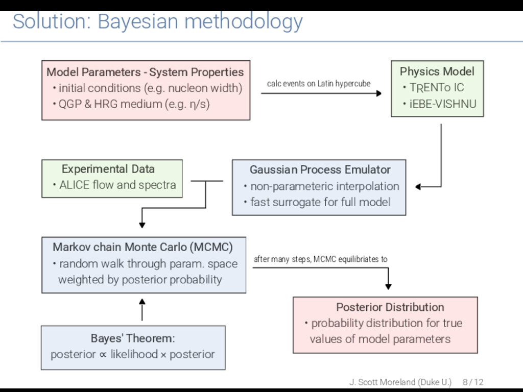
12. Solution: Bayesian methodology Model Parameters - System Properties • initial conditions (e.g. nucleon width) • QGP & HRG medium (e.g. η/s) Physics Model • TRENTo IC • iEBE-VISHNU Experimental Data • ALICE flow and spectra Gaussian Process Emulator • non-parameteric interpolation • fast surrogate for full model Markov chain Monte Carlo (MCMC) • random walk through param. space weighted by posterior probability Bayes' Theorem: posterior ∝ likelihood × posterior Posterior Distribution • probability distribution for true values of model parameters after many steps, MCMC equilibriates to calc events on Latin hypercube J. Scott Moreland (Duke U.) 8 / 12
13. Calibrating the model: before and after 100 101 102 103 Training data π± K± p¹ p Yields dN/dy 0.0 0.5 1.0 1.5 π± K± p¹ p Mean pT [GeV] 0.00 0.03 0.06 0.09 v2 v3 v4 Flow cumulants vn {2} 0 10 20 30 40 50 60 70 Centrality % 100 101 102 103 Posterior samples π± K± p¹ p 0 10 20 30 40 50 60 70 Centrality % 0.0 0.5 1.0 1.5 π± K± p¹ p 0 10 20 30 40 50 60 70 Centrality % 0.00 0.03 0.06 0.09 v2 v3 v4 Top: run model (×104 events) at each design point (×300 evals) Bottom: emulator predictions for 100 samples from the posterior J. Scott Moreland (Duke U.) 9 / 12
14. Calibrated to identified particles 100 130 160 norm -1.0 0.0 1.0 p 0.8 1.5 2.2 k 0.4 0.7 1.0 w [fm] 0.0 0.15 0.3 η/s min 0.0 1.0 2.0 η/s slope† 0.0 1.0 2.0 ζ/s norm 100 130 160 norm 0.14 0.15 0.16 Tsw [GeV] -1.0 0.0 1.0 p 0.8 1.5 2.2 k 0.4 0.7 1.0 w [fm] 0.0 0.15 0.3 η/s min 0.0 1.0 2.0 η/s slope† 0.0 1.0 2.0 ζ/s norm 0.14 0.15 0.16 Tsw [GeV] Calibrated to charged particles
15. Calibrated to identified particles 100 130 160 norm -1.0 0.0 1.0 p 0.8 1.5 2.2 k 0.4 0.7 1.0 w [fm] 0.0 0.15 0.3 η/s min 0.0 1.0 2.0 η/s slope† 0.0 1.0 2.0 ζ/s norm 100 130 160 norm 0.14 0.15 0.16 Tsw [GeV] -1.0 0.0 1.0 p 0.8 1.5 2.2 k 0.4 0.7 1.0 w [fm] 0.0 0.15 0.3 η/s min 0.0 1.0 2.0 η/s slope† 0.0 1.0 2.0 ζ/s norm 0.14 0.15 0.16 Tsw [GeV] Calibrated to charged particles -1.0 -0.5 0.0 0.5 1.0 p KLN EKRT WN Entropy deposition parameter Generalized mean parametrization: dS/dy ∝ Tp A +Tp B 2 1/p
16. Calibrated to identified particles 100 130 160 norm -1.0 0.0 1.0 p 0.8 1.5 2.2 k 0.4 0.7 1.0 w [fm] 0.0 0.15 0.3 η/s min 0.0 1.0 2.0 η/s slope† 0.0 1.0 2.0 ζ/s norm 100 130 160 norm 0.14 0.15 0.16 Tsw [GeV] -1.0 0.0 1.0 p 0.8 1.5 2.2 k 0.4 0.7 1.0 w [fm] 0.0 0.15 0.3 η/s min 0.0 1.0 2.0 η/s slope† 0.0 1.0 2.0 ζ/s norm 0.14 0.15 0.16 Tsw [GeV] Calibrated to charged particles 0.8 1.0 1.2 1.4 1.6 1.8 2.0 2.2 k Proton multiplicity fluctuations Random Gamma nucleon weights: P(γ | k) = kk Γ(k) γk−1e−kγ TA(x, y) = Npart,A i=1 γiTp(x − xi, y − yi)
17. Calibrated to identified particles 100 130 160 norm -1.0 0.0 1.0 p 0.8 1.5 2.2 k 0.4 0.7 1.0 w [fm] 0.0 0.15 0.3 η/s min 0.0 1.0 2.0 η/s slope† 0.0 1.0 2.0 ζ/s norm 100 130 160 norm 0.14 0.15 0.16 Tsw [GeV] -1.0 0.0 1.0 p 0.8 1.5 2.2 k 0.4 0.7 1.0 w [fm] 0.0 0.15 0.3 η/s min 0.0 1.0 2.0 η/s slope† 0.0 1.0 2.0 ζ/s norm 0.14 0.15 0.16 Tsw [GeV] Calibrated to charged particles 0.4 0.5 0.6 0.7 0.8 0.9 1.0 w [fm] Nucleon width Gaussian nucleon thickness: Tp(x, y) = 1 2πw2 e−(x2+y2)/(2w2)
18. Calibrated to identified particles 100 130 160 norm -1.0 0.0 1.0 p 0.8 1.5 2.2 k 0.4 0.7 1.0 w [fm] 0.0 0.15 0.3 η/s min 0.0 1.0 2.0 η/s slope† 0.0 1.0 2.0 ζ/s norm 100 130 160 norm 0.14 0.15 0.16 Tsw [GeV] -1.0 0.0 1.0 p 0.8 1.5 2.2 k 0.4 0.7 1.0 w [fm] 0.0 0.15 0.3 η/s min 0.0 1.0 2.0 η/s slope† 0.0 1.0 2.0 ζ/s norm 0.14 0.15 0.16 Tsw [GeV] Calibrated to charged particles 0.15 0.20 0.25 0.30 Temperature [GeV] 0.0 0.2 0.4 0.6 η/s KSS bound 1/4π Prior range Posterior median 90% CI Shear viscosity parametrization: (η/s)(T) = (η/s)min +(T−Tc)(η/s)slope
19. Running the model with high probability parameters Choose high probability model parameters from Bayesian posterior (right) Run full hybrid model using high probability parameters (bottom) Initial condition QGP medium norm 120. η/s min 0.08 p 0.0 η/s slope 0.85 GeV−1 k 1.5 ζ/s norm 1.25 w 0.43 fm Tsw 0.148 GeV 100 101 102 103 104 π± K± p¹ p Nch ×5 solid: identified dashed: charged Yields dN/dy, dNch /dη 0 10 20 30 40 50 60 70 Centrality % 0.8 1.0 1.2 Model/Exp 0.0 0.4 0.8 1.2 π± K± p¹ p Mean pT [GeV] 0 10 20 30 40 50 60 70 Centrality % 0.8 1.0 1.2 0.00 0.03 0.06 0.09 v2 v3 v4 Flow cumulants vn {2} 0 10 20 30 40 50 60 70 Centrality % 0.8 1.0 1.2 J. Scott Moreland (Duke U.) 11 / 12
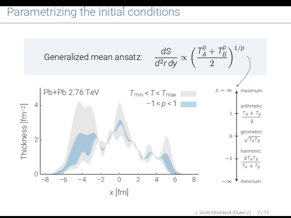
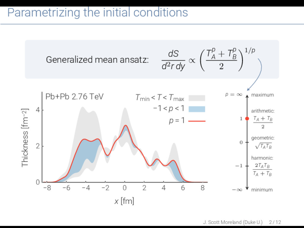
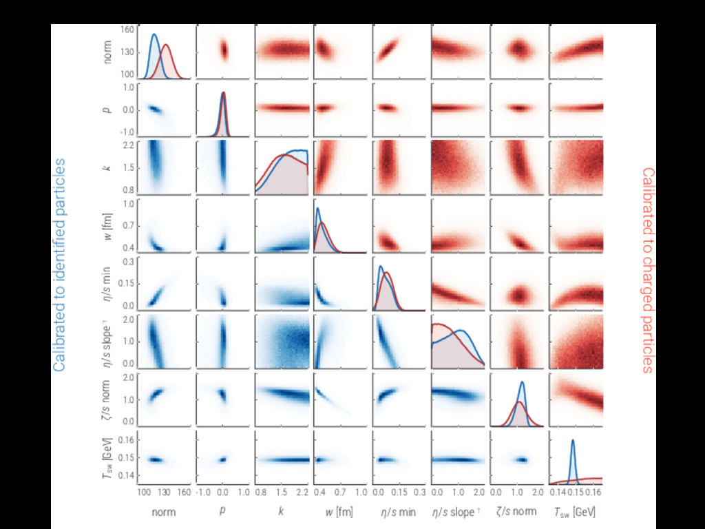
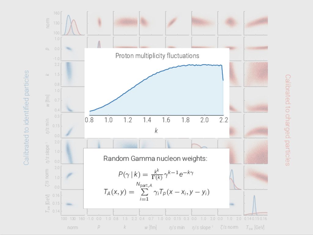
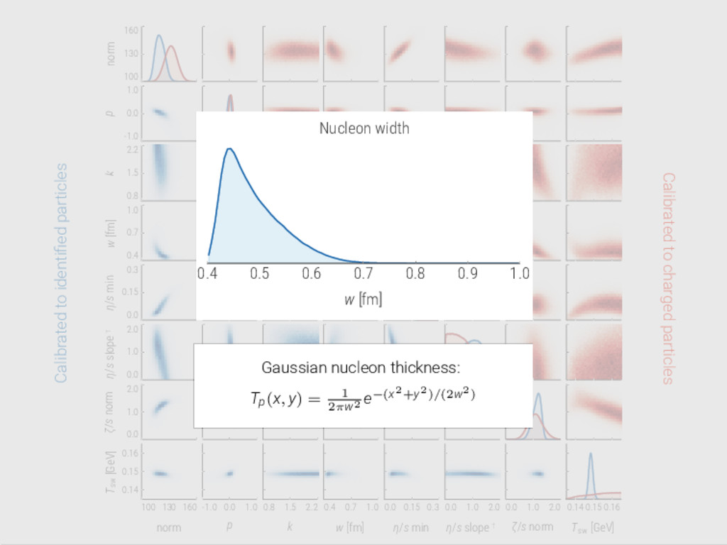
20. Conclusions Initial condition properties Yields, mean pT and flows impose strong constraints on IC. Entropy deposition mimicked by dS/dy ∼ √ TA TB Data strongly prefers small nucleon width w ≈ 0.4–0.6 fm! A+A collisions weakly sensitive to p+p mult. fluctuations Preferred initial conditions similar to EKRT, IP-Glasma Hydrodynamic transport properties First quantitative credibility interval on (η/s)(T)! Data prefer non-zero bulk viscosity Hydro-to-micro Tsw determined by relative species yields TRENTo is publicly available at qcd.phy.duke.edu/trento More in the pre-print arXiv:1605.03954
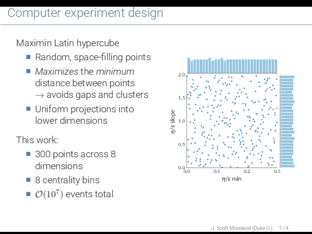
21. Computer experiment design Maximin Latin hypercube Random, space-filling points Maximizes the minimum distance between points → avoids gaps and clusters Uniform projections into lower dimensions This work: 300 points across 8 dimensions 8 centrality bins O(107) events total 0.0 0.1 0.2 0.3 η/s min 0.0 0.5 1.0 1.5 2.0 η/s slope J. Scott Moreland (Duke U.) 1 / 4
22. TRENTo 3D, work in progress... Extend to forward/backward rapidities while maintaining mid-rapidity result: s(x⊥, η) = s(x⊥, η = 0) · f(x⊥, η) Parametrize f(x⊥, η) by first few cumulants, mean std skewness kurtosis µ(x⊥) σ(x⊥) γ(x⊥) κ(x⊥) Reconstruct f(η) by F−1 cumulant generating function, F−1 exp(iµk − σ2 2 k2 + iγk3 − κk4) 1200 1600 2000 2400 dNch /dη 0—5% 900 1200 1500 1800 5—10% 600 900 1200 1500 10—20% 400 600 800 1000 20—30% 300 400 500 600 30—40% −3 0 3 η 200 300 400 dNch /dη 40—50% −3 0 3 η 80 120 160 200 50—60% −3 0 3 η 40 60 80 100 60—70% −3 0 3 η 20 30 40 50 70—80% −3 0 3 η 9 12 15 18 80—90% Pb+Pb
23. TRENTo 3D, work in progress... Extend to forward/backward rapidities while maintaining mid-rapidity result: s(x⊥, η) = s(x⊥, η = 0) · f(x⊥, η) Parametrize f(x⊥, η) by first few cumulants, mean std skewness kurtosis µ(x⊥) σ(x⊥) γ(x⊥) κ(x⊥) Reconstruct f(η) by F−1 cumulant generating function, F−1 exp(iµk − σ2 2 k2 + iγk3 − κk4) 40 60 dNch /dη 0—1% 30 40 50 60 1—5% 20 30 40 50 5—10% 20 30 40 10—20% −2 0 2 η 20 30 dNch /dη 20—30% −2 0 2 η 20 30 30—40% −2 0 2 η 8 12 16 20 40—60% −2 0 2 η 4 6 8 10 12 60—90% p+Pb
24. Comparing to the IP-Glasma model 0 2 4 6 8 10 12 14 Impact parameter b [fm] 0.0 0.1 0.2 0.3 0.4 0.5 0.6 εn ε2 ε3 TRENTO p = 0 ± 0. 1 IP-Glasma IP-Glasma: multi-stage dynamical model, simple analytic mapping unknown. Analyze effective mapping via eccentricity harmonics εn (left). Work ongoing: determine IP-Glasma effective mapping for direct comparison with TRENTo parametrization J. Scott Moreland (Duke U.) 3 / 4
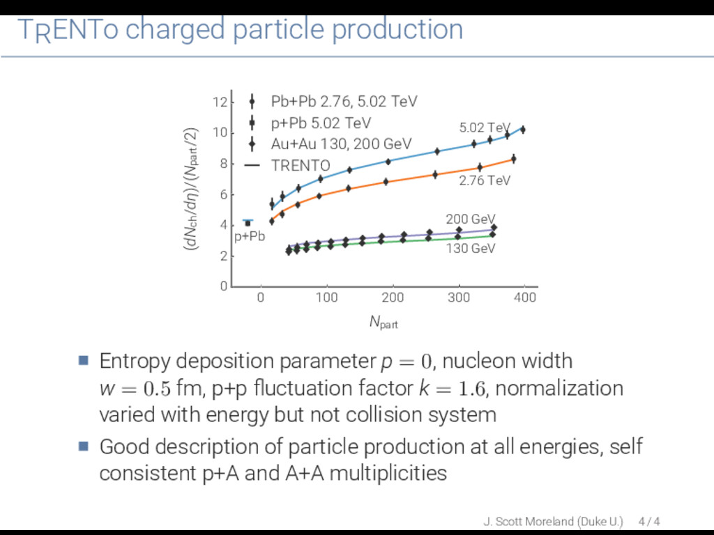
25. TRENTo charged particle production 0 100 200 300 400 Npart 0 2 4 6 8 10 12 (dNch /dη)/(Npart /2) p+Pb 5.02 TeV 2.76 TeV 200 GeV 130 GeV Pb+Pb 2.76, 5.02 TeV p+Pb 5.02 TeV Au+Au 130, 200 GeV TRENTO Entropy deposition parameter p = 0, nucleon width w = 0.5 fm, p+p fluctuation factor k = 1.6, normalization varied with energy but not collision system Good description of particle production at all energies, self consistent p+A and A+A multiplicities J. Scott Moreland (Duke U.) 4 / 4