Mathias Fuchs - How to measure the performance of a machine learning algorithm

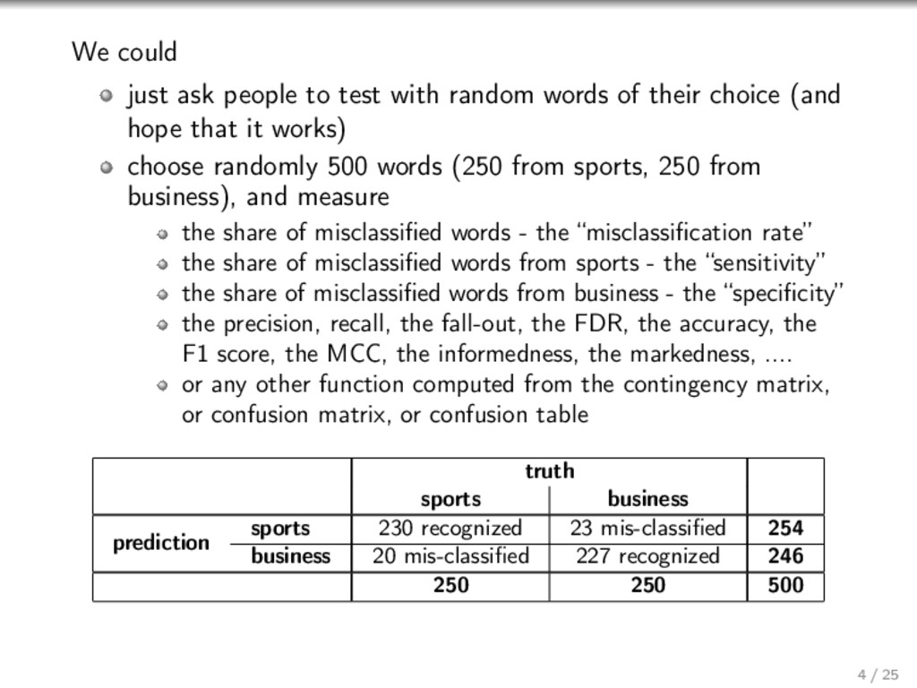
Machine learning has seen an impressing boom in the past years. In practice, every learning algorithm has to prove its worth by better classification/prediction performance than previous algorithms. However, obvious performance measures such as the misclassification rate and so on suffer a high variability across data-sets or even re-sampling iterations. Thus, it is a challenging problem to assess the performance reliably, and its importance has been given surprisingly little attention in literature and practice. I will talk about the usual performance measures such as misclassification rate, AUC or mean squared error etc. I will explain cross-validation and its pitfalls. Finally, I will show you a new method to estimate the variability of the performance estimators in a general and statistically correct way.

Transcript

1. How to measure a machine learning algorithm’s performance Mathias Fuchs Munich Datageeks Meetup 06 - 04 - 2014 1 / 25
2. Outline 1 What is the “performance” of a machine learning algorithm and why does one need to measure it? 2 Which are the main methods? which are the peculiarities of unbalanced datasets? 3 What is the variance of the performance measures, and how do we estimate it? 4 Benchmarking methods and statistical hypothesis tests 2 / 25
3. Example Simple text classification: classify the topic of user input words Is it good? Is it bad? Is it “better” than algorithm XYZ? 3 / 25
4. We could just ask people to test with random words of their choice (and hope that it works) choose randomly 500 words (250 from sports, 250 from business), and measure the share of misclassified words - the “misclassification rate” the share of misclassified words from sports - the “sensitivity” the share of misclassified words from business - the “specificity” the precision, recall, the fall-out, the FDR, the accuracy, the F1 score, the MCC, the informedness, the markedness, .... or any other function computed from the contingency matrix, or confusion matrix, or confusion table truth sports business sports 230 recognized 23 mis-classified 254 prediction business 20 mis-classified 227 recognized 246 250 250 500 4 / 25
5. t(table(truth, predictions)) ## truth ## predictions 0 1 ## 0 230 23 ## 1 20 227 5 / 25
6. Assuming that 450 words were correctly classified: binom.test(n = 500, x = 50) ## ## Exact binomial test ## ## data: 50 and 500 ## number of successes = 50, number of trials = 500, p-value ## 2.2e-16 ## alternative hypothesis: true probability of success is no ## 95 percent confidence interval: ## 0.07514 0.12971 ## sample estimates: ## probability of success ## 0.1 6 / 25
7. Thus, we could be quite sure that the “true” misclassification rate is between 8% and 13 %, and “quite sure” means that this method is guaranteed to yield an interval containing the true value with a probability of 95%. More generally, one could define a so-called loss function l(x, y) so that the parameter of interest (sensitivity, specificity, etc.) is the average loss function. truth <- c(rep(0, 250), rep(1, 250)) # simulated predictions predictions <- c( rbinom(250, 1, p =.1), rbinom(250, 1, p = .9) ) loss <- function(x) as.numeric(x[1] != x[2]) 7 / 25
8. observedLosses <- apply( rbind(truth, predictions), 2, loss ) t.test(observedLosses) ## ## One Sample t-test ## ## data: observedLosses ## t = 7.279, df = 499, p-value = 1.311e-12 ## alternative hypothesis: true mean is not equal to 0 ## 95 percent confidence interval: ## 0.07009 0.12191 ## sample estimates: ## mean of x ## 0.096 8 / 25
9. What if the classification algorithm returns predictions on a metric scale instead of binary values? Examples: naive Bayes classifier, logistic regression, ... Then, the measure of choice is the AUC ( = are under the curve) Each number defines a cut-off, thus, a false and a true positive rate. This is is strongly monotonous function, the ROC curve 9 / 25
10. Variance 10 / 25
11. Variance V(X) = E(X − E(X))2 = E(X2 − 2XE(X) + E(X)2) = E(X2) − 2E(X)2 + E(X)2 = E(X2) − E(X)2 Θ := true loss or true AUC; or differences thereof if two methods are to be compared. Θ: our estimator, calculated from the data. Take X := Θ V(Θ) = Θ2 − Θ2 The first term is always easy, the second is a little harder. 11 / 25
12. The normalized AUC is the probability that two random observations (x1, y1), (x2, y2) of different classes satisfy sign (y2 − y1) = sign (y2 − y1) The AUC is somewhat, but not extremely more difficult to handle than a loss defined by a loss function. Having calculated the AUC on some testing data, how do we set up a confidence interval? Short answer: Obtain an unbiased variance estimator on each quadruple of observations by multiplying the AUC on the first pair with that of the second pair and substracting the square of the AUC. Repeat for all quadrupels. The width of the confidence interval is the square root of the variance estimator, rescaled by a factor determined by the significance level. 12 / 25
13. Remark: If we want to compare two classification algorithms, there are two Θ and Θ , and V(Θ − Θ ) = V(Θ) + V(Θ ) − 2Cov(Θ, Θ ) 13 / 25
14. Back to loss functions. So far, we have supposed the training data to be fixed. What happens if we have to handle new training data every day? Example: we supply an image classification tool, and every customer comes up with his own classification task. Thus, we now put the classification algorithm under investigation, rather than just a resulting prediction rule. 14 / 25
15. Definition The conditional loss is the true loss of the prediction rule obtained by training on the training data (i.e. for one customer). Definition The unconditional loss is the true loss of the learning algorithm in general, for the “average” training data. For misclassification, it is equal to the misclassification loss if training and testing data are simultaneously and randomly drawn from the population. Even though these two viewpoints are quite different, the conditional one is a special case of the unconditional one, obtained by supposing the special case of zero training data size. 15 / 25
16. Does that seem complicated? Goal: to set up a confidence interval for the unconditional error rate. 16 / 25
17. Method 1 - using cross-validation Randomly divide the data into K subsets, K = 5. Do a loop 1, . . . , K. In each iteration, compute the observed losses when using the K-th part of the data as testing set, and the rest as training set. Compute the confidence interval as above from these observed losses. Thus, there are no overlaps within testing data; but many overlaps between testing and training data, and within training data. (Why is this better than vice versa?) If interested only in the best estimator for the loss, one may repeat the procedure for different splits, and average the results. CV is, more or less, the standard approach, at least for the loss function itself. Also works for AUC (to some degree). 17 / 25
18. What are the problems? 1 No one knows how to choose K. 2 The entire procedure depends on the random splits! 3 The observed losses are strongly correlated because of the said overlaps. This “tricks” our t-test into thinking they are so close together because of a strong “signal”. Thus, the t-test is severly wrong. 18 / 25
19. My thoughts 1 There is no universal solution for all classifiers. However, the impact of varying K is in most cases not very strong. Some theory exists for linear regression. 2 As far as the loss is concerned, the problem can be solved by repeating, repeating, repeating the procedure until the average converges. 3 This is the topic of our paper: 19 / 25
20. Mathias Fuchs, Roman Hornung, Riccardo De Bin, Anne-Laure Boulesteix A U-statistic estimator for the variance of resampling-based error estimators Technical Report Number 148, 2013 Department of Statistics University of Munich http://www.stat.uni-muenchen.de 20 / 25
21. Let n be the sample size, g = n − n/K the learning set size. Let Θ be the average of all observed losses, taken across all possible learning sets. Question: What is the variance of Θ? This is important: suppose we know – somehow – the variance v = V(Θ). Then, the confidence interval is [Θ ± √ vφ−1(1 − α/2)] Thus, how can one estimate this variance? 21 / 25
22. Method 2 - using leave-p-out-validation Theorem The best variance estimator is given by the following procedure: 1 Compute Θ as above. 2 For each pairs of learning sets (each of size g) and test observations, all disjoint, compute a prediction rule on each of the two learning sets and evaluate each on one of the two test observations. Multiply the two numbers. Repeat for many subsets of size 2g + 2 and average out. This gives an estimator for Θ2. 3 Then, v = Θ2 − Θ2 Proof. The variance is a U-statistic. 22 / 25
23. How often to “repeat, repeat, repeat, . . . ”? Theorem Let Φ be a function whose expectation value is to be re-sampled (such as the loss to compute Θ, or the product of two losses, to compute Θ2). Let −1 ≤ Φ ≤ 1, let T ∗ be a collection of N randomly drawn (fixed size) subsets of {1, . . . , n}. Let Φ(T ∗) be the result of evaluating on the sub-sample T ∗. Then the probability of approximation error at least δ > 0 is bounded by pr(|Φ(T ∗) − Φ(T )| ≥ δ) ≤ 2 exp −δ2N/2 . Rule of thumb: After 102d+1 iterations, you know d digits after the decimal point! For cheaters: check the t-test confidence interval calculated from the re-sampling iterations ... it will most likely tell you where the average will finally come to rest! 23 / 25
24. Theorem Then (Θ − Θ)v−1/2 converges in distribution to N(0, 1) as g remains fixed, n → ∞. Corollary The confidence interval [Θ ± √ vφ−1(1 − α/2)] is asymptotically exact (“valid”), as is the statistical hypothesis test of the null hypothesis Θ = 0. Therefore, the confidence interval from Method 2 is correct. 24 / 25
25. Thanks for your attention! www.biostats.de fuchs@ibe.med.uni-muenchen.de 25 / 25