AI Concepts - MCP Neurons

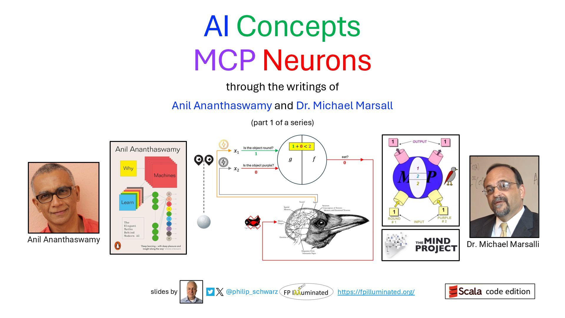
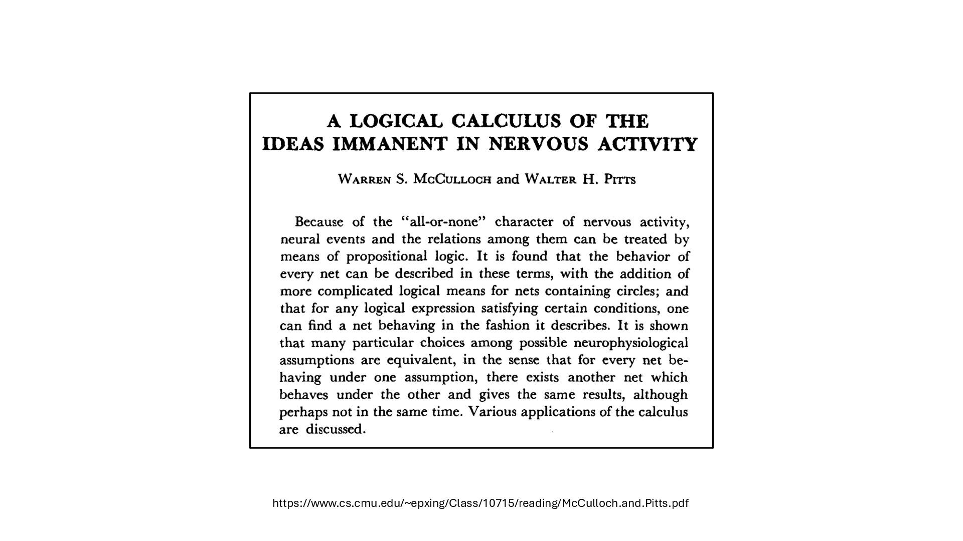
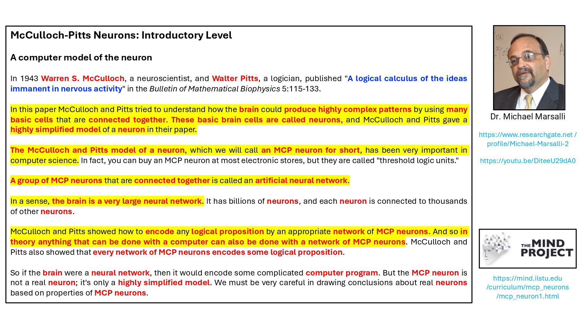
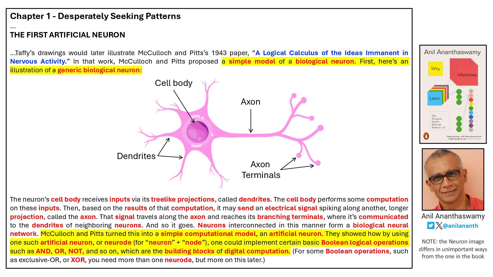
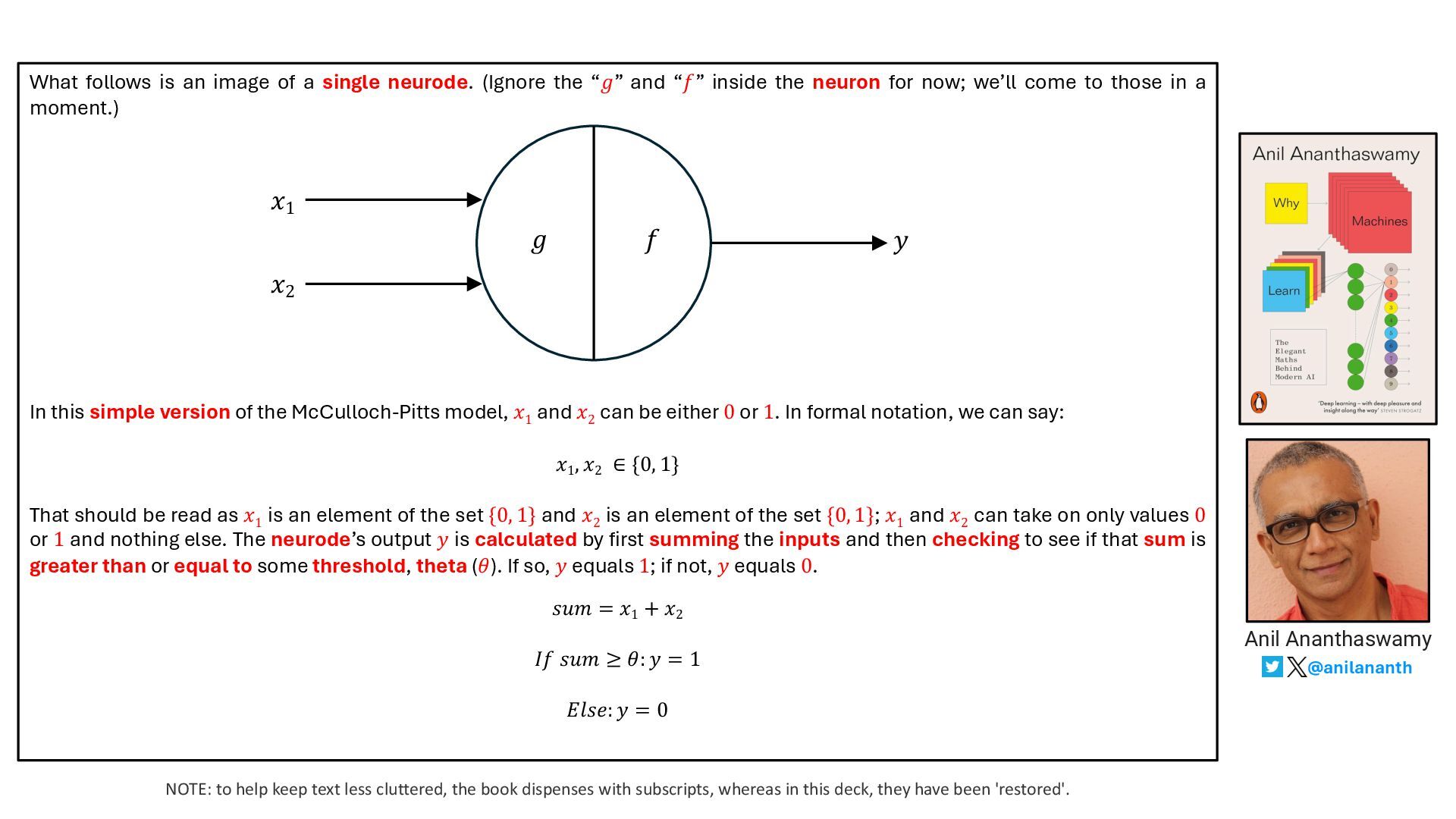
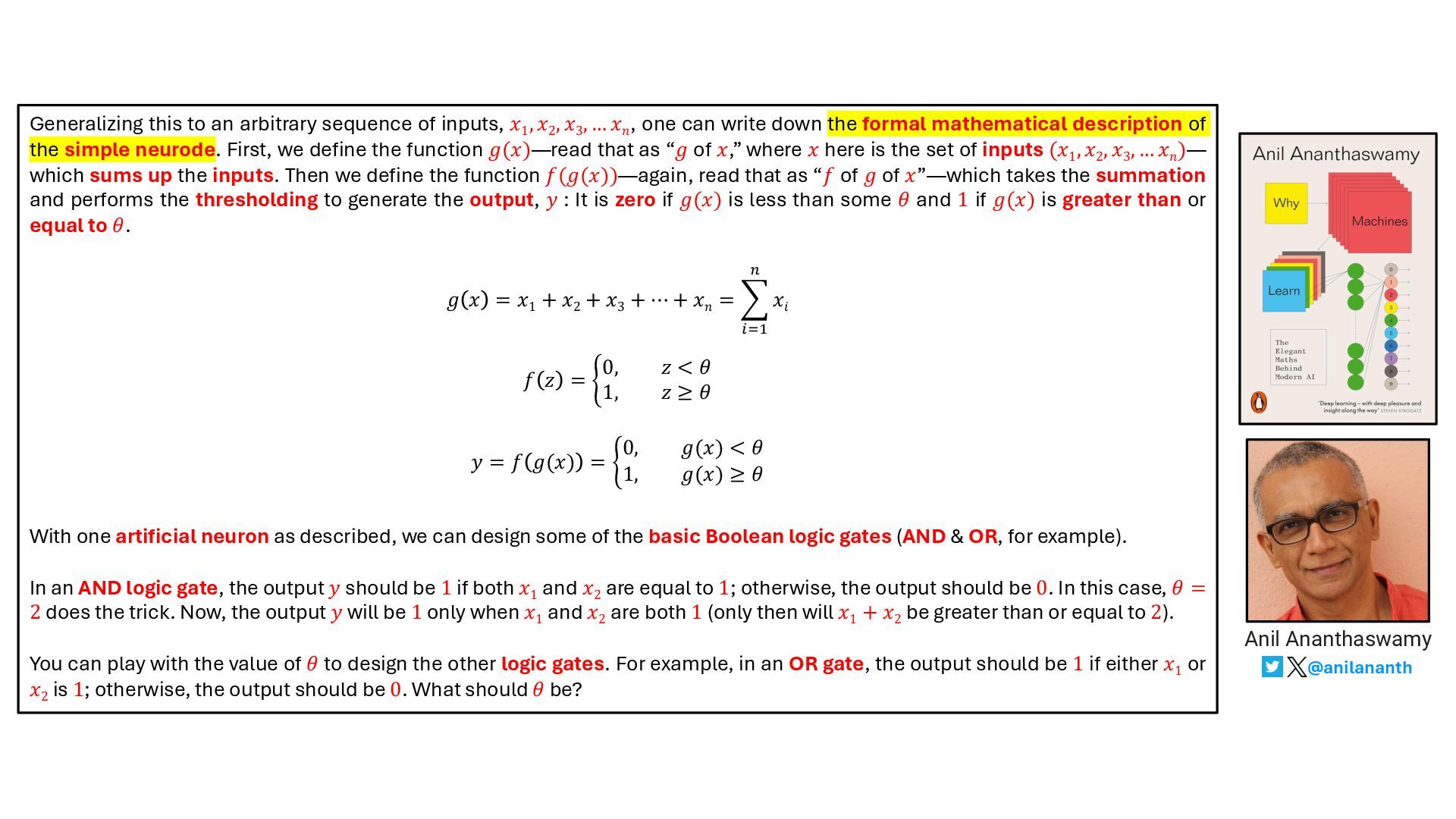
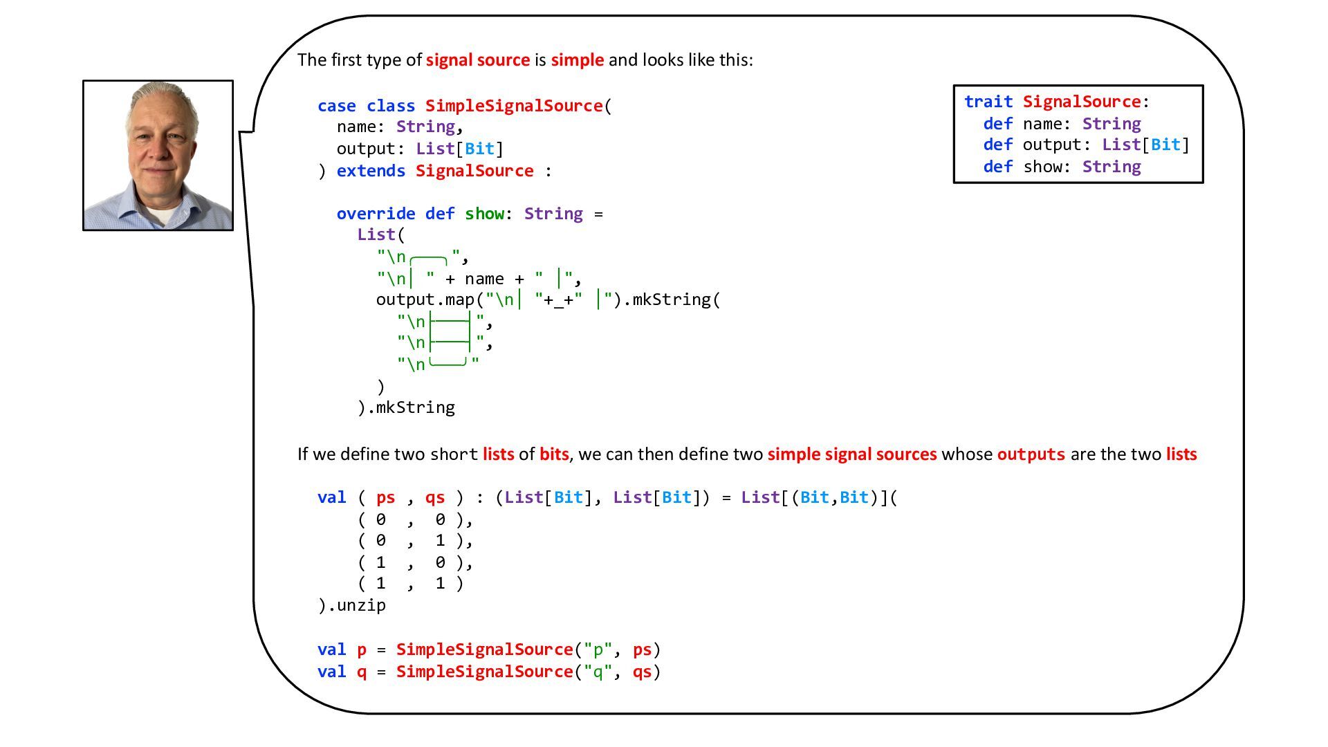
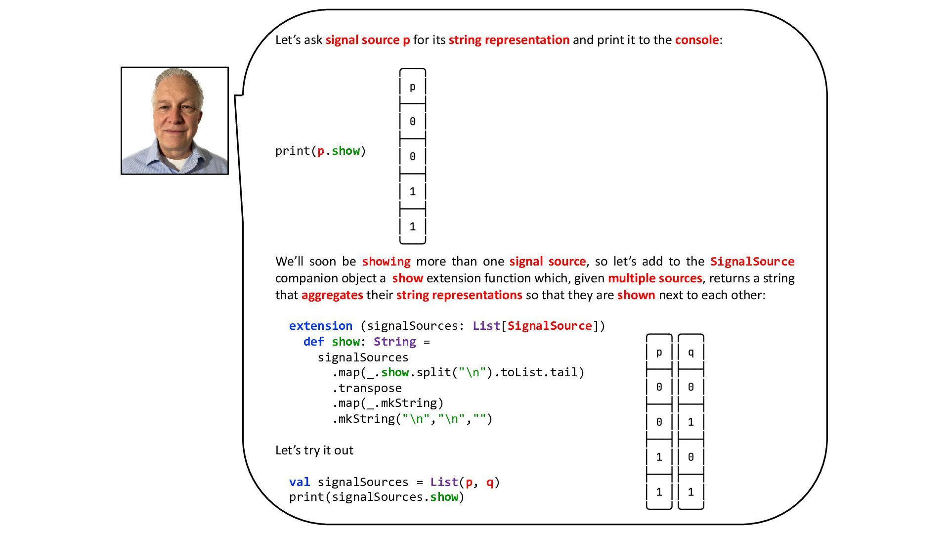
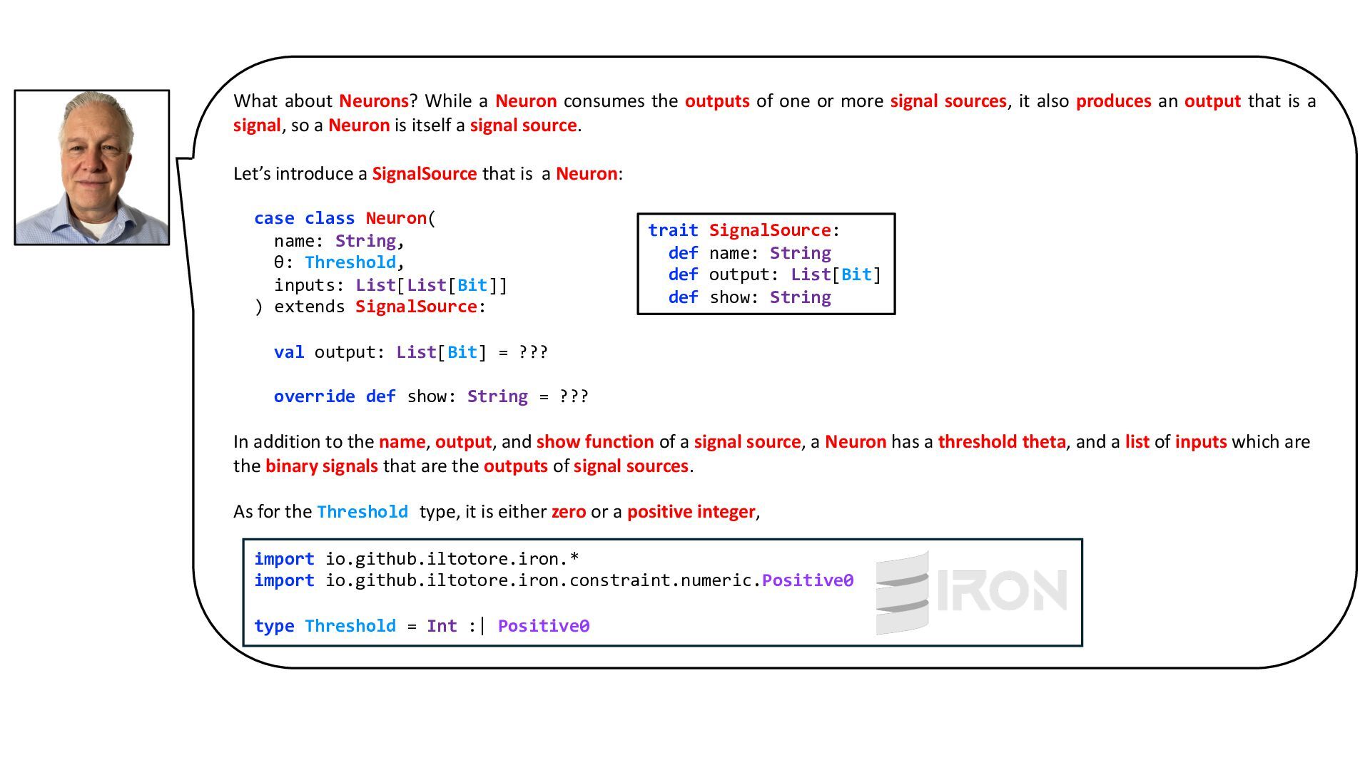
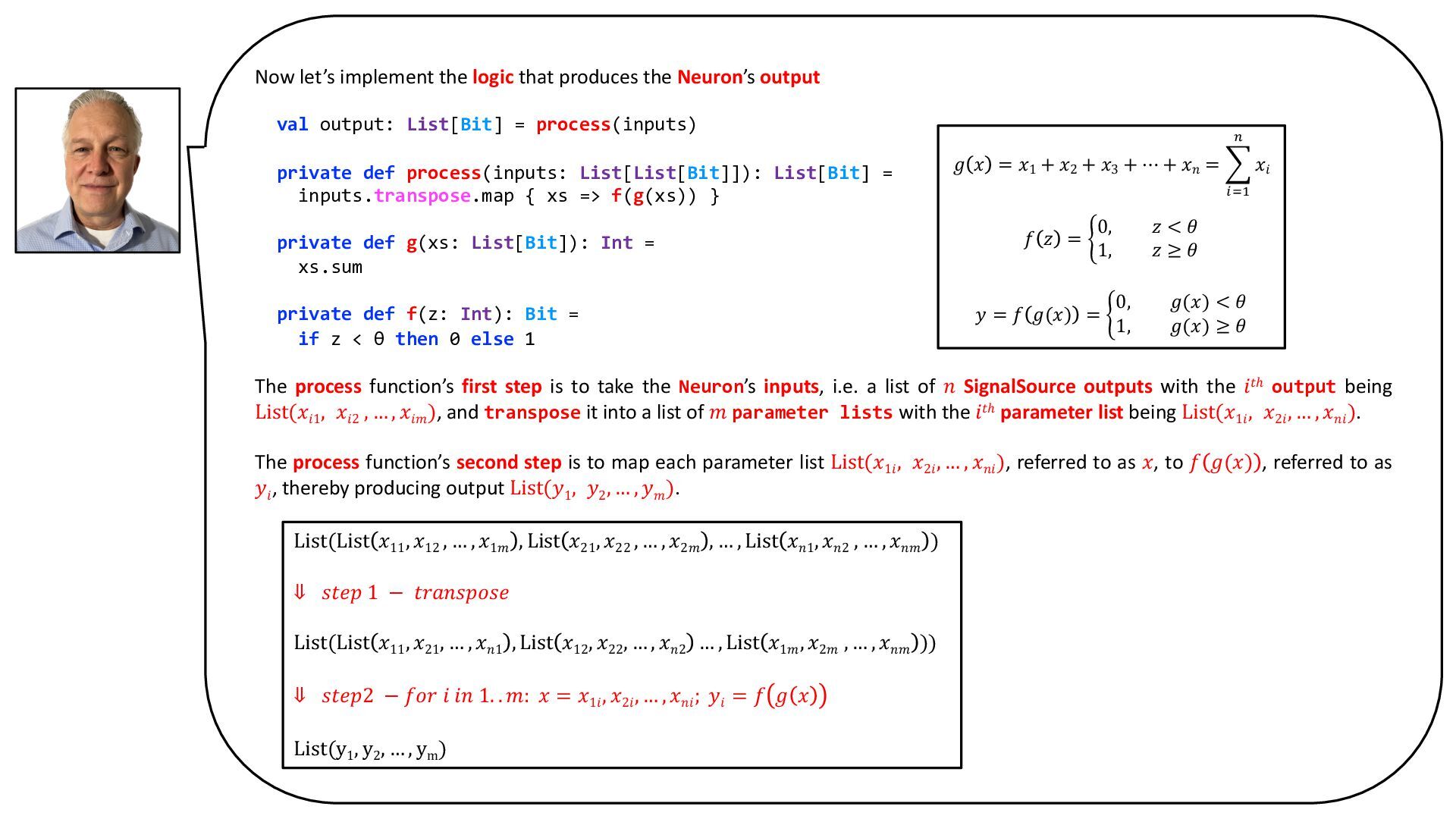
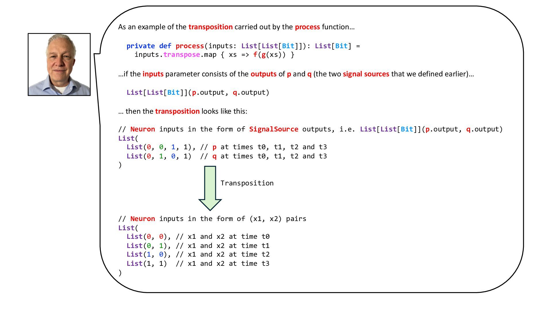
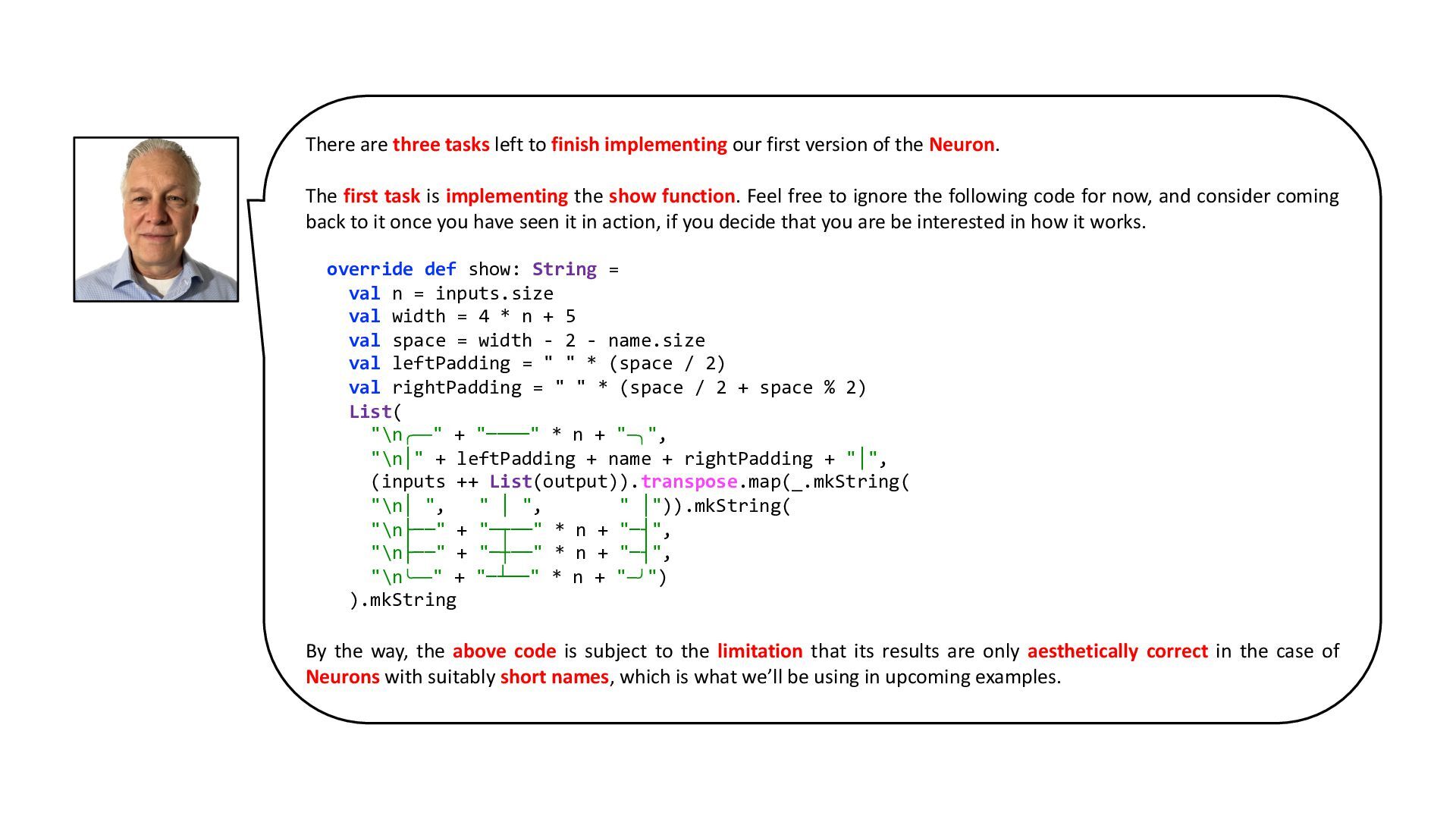
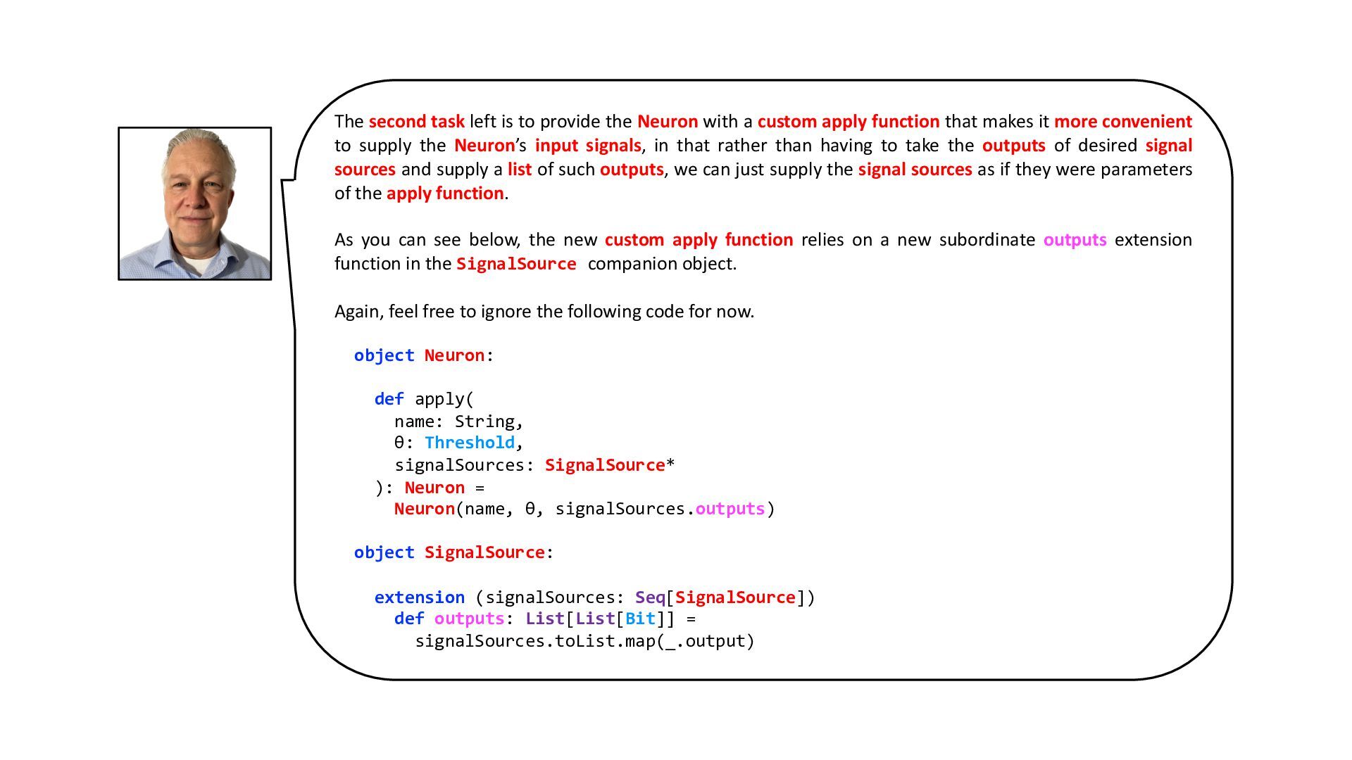
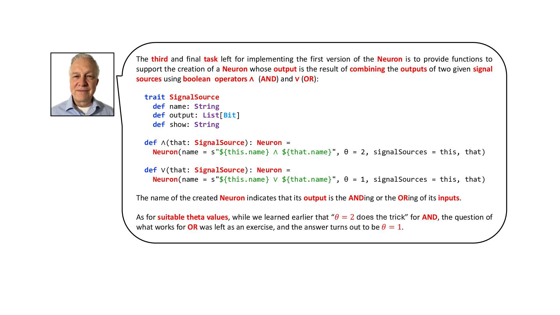
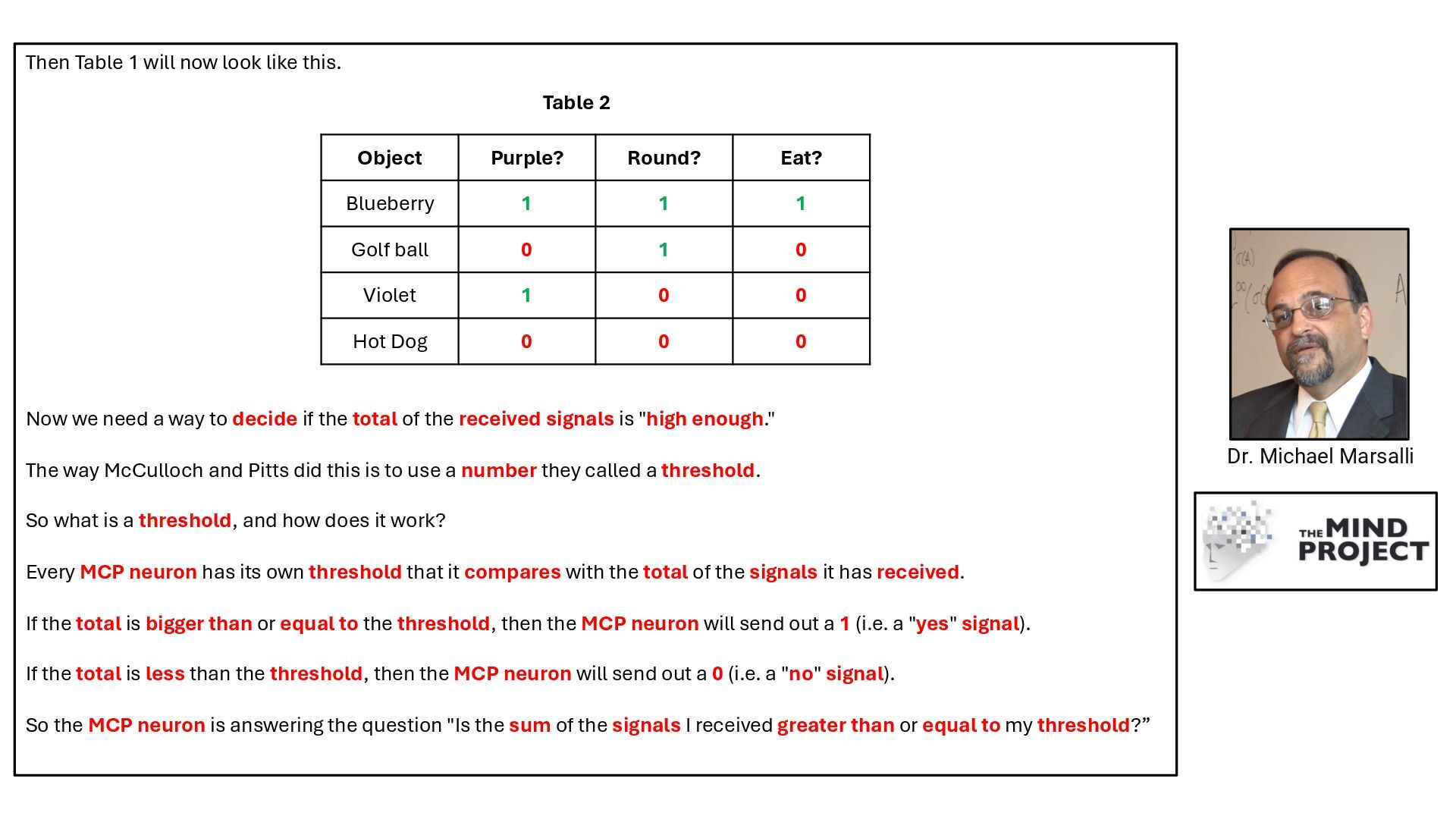
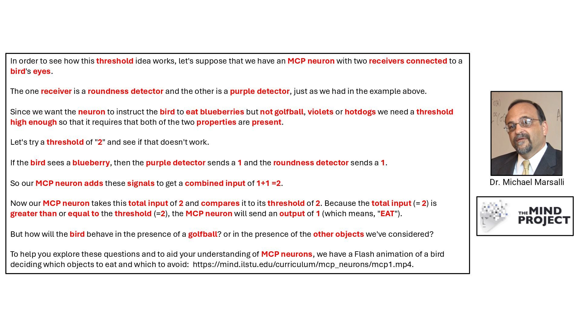
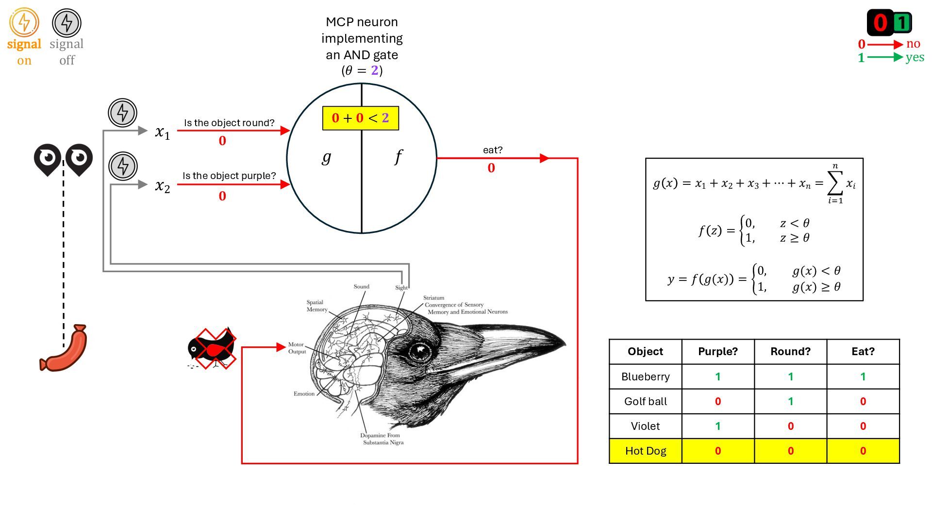
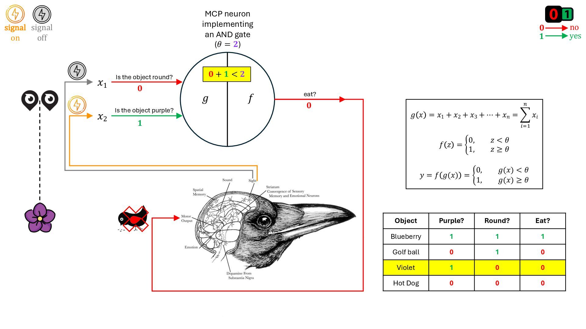
In this first deck in the series on AI concepts we look at the MCP Neuron.

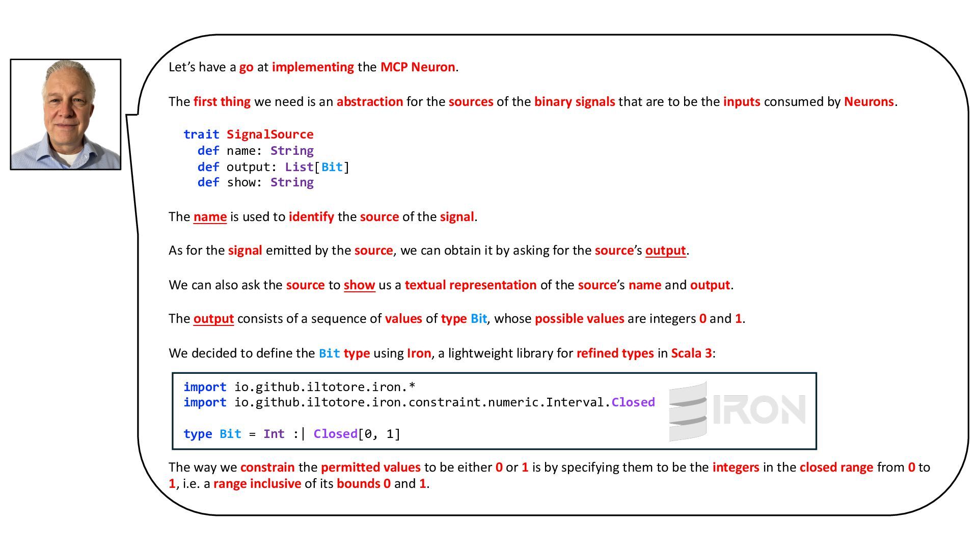
After learning its formal mathematical definition, we write a program that allows us to:
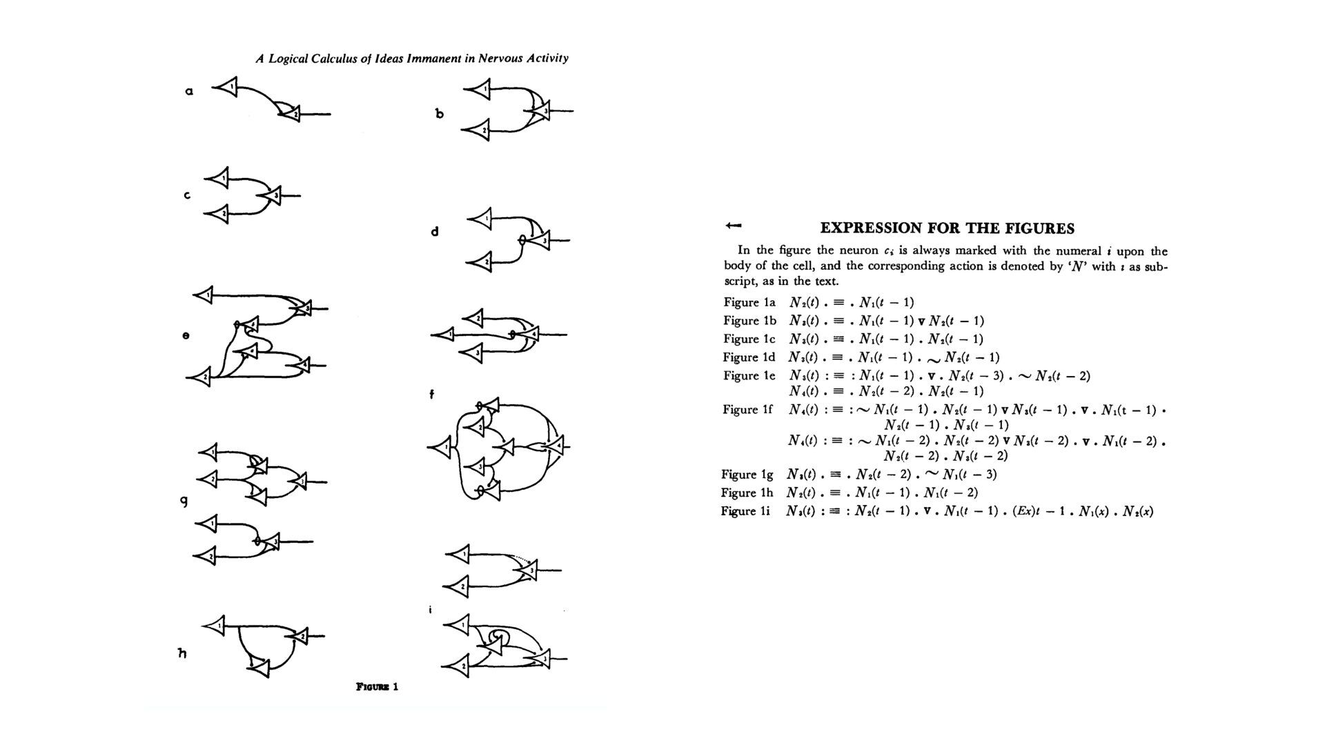
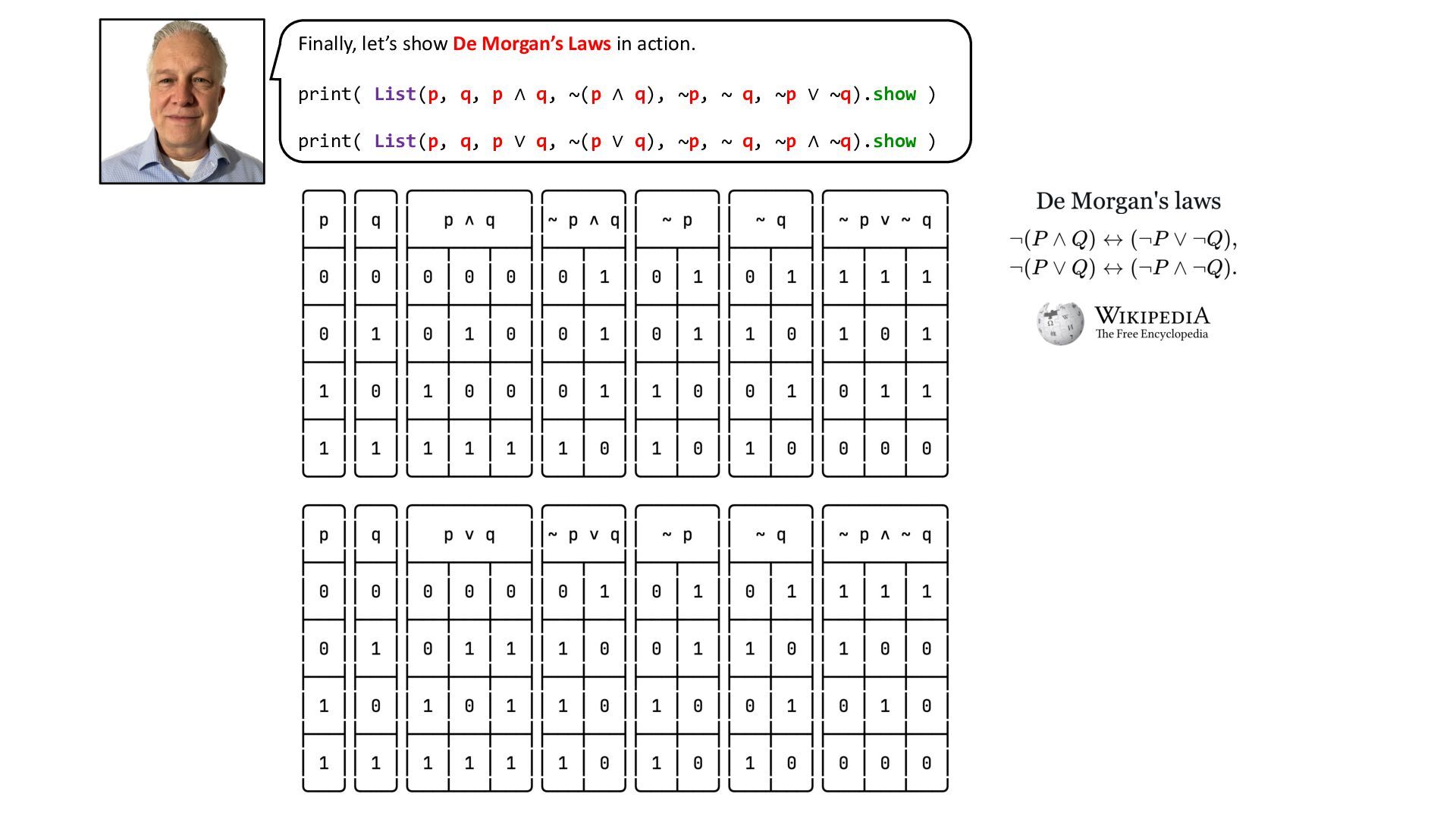
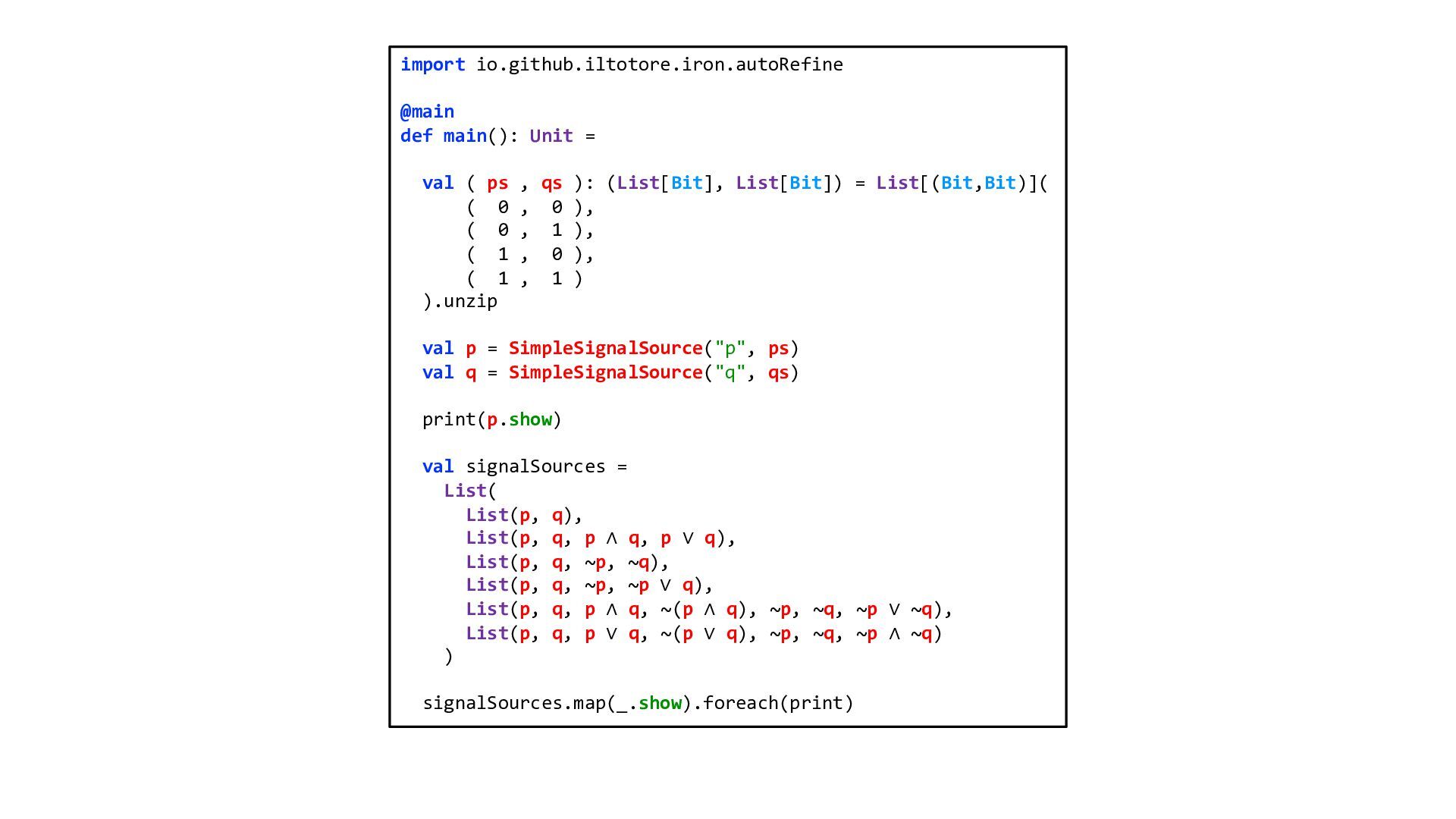
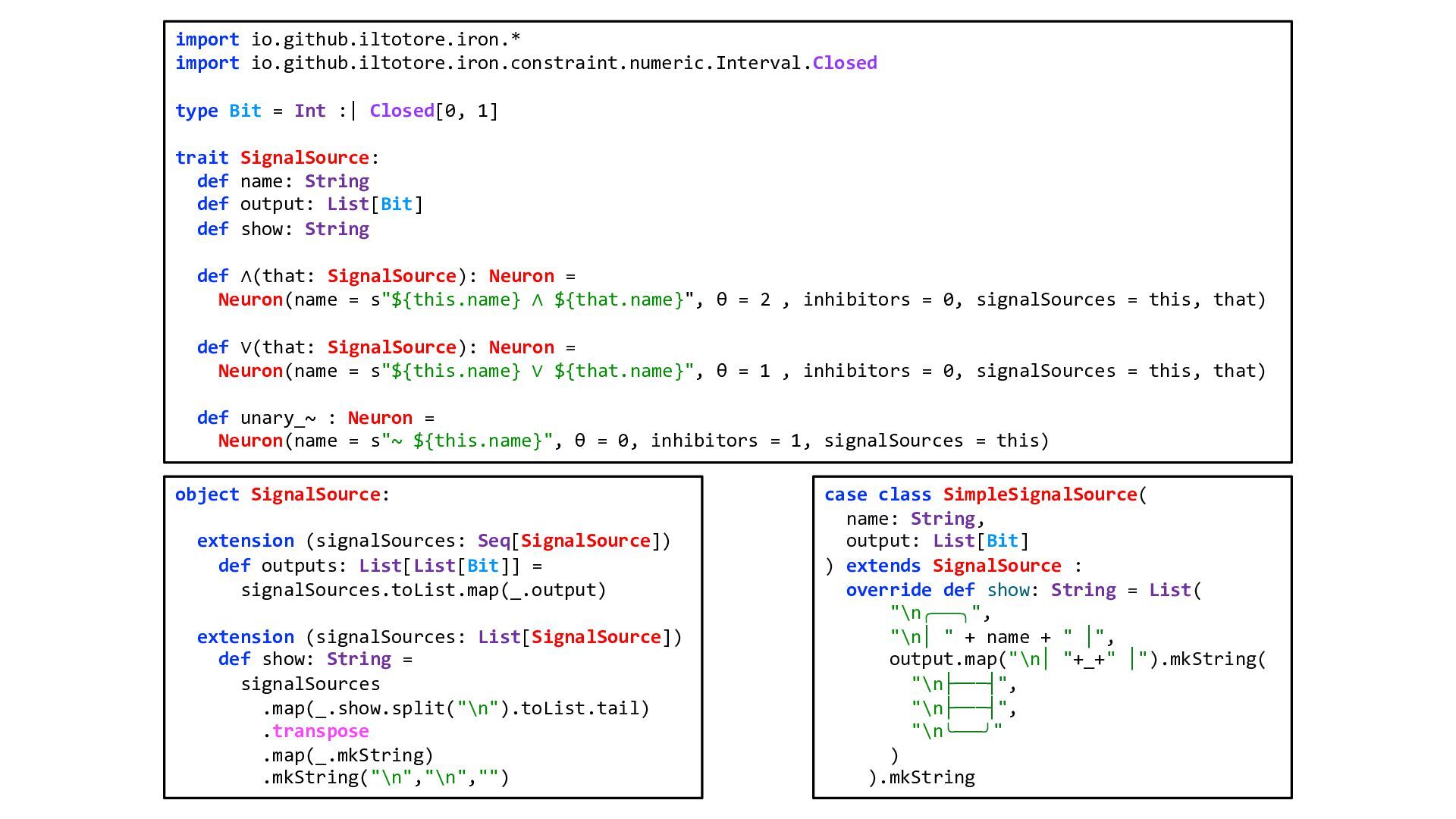
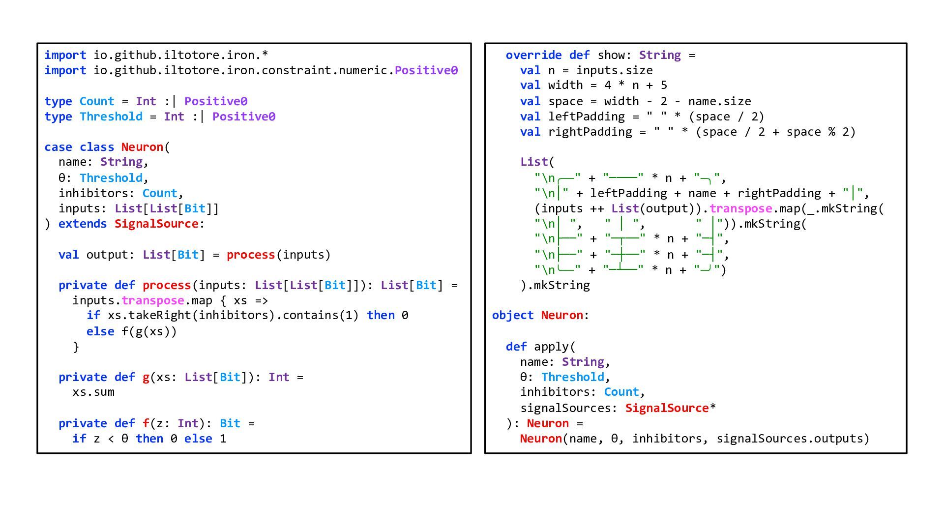
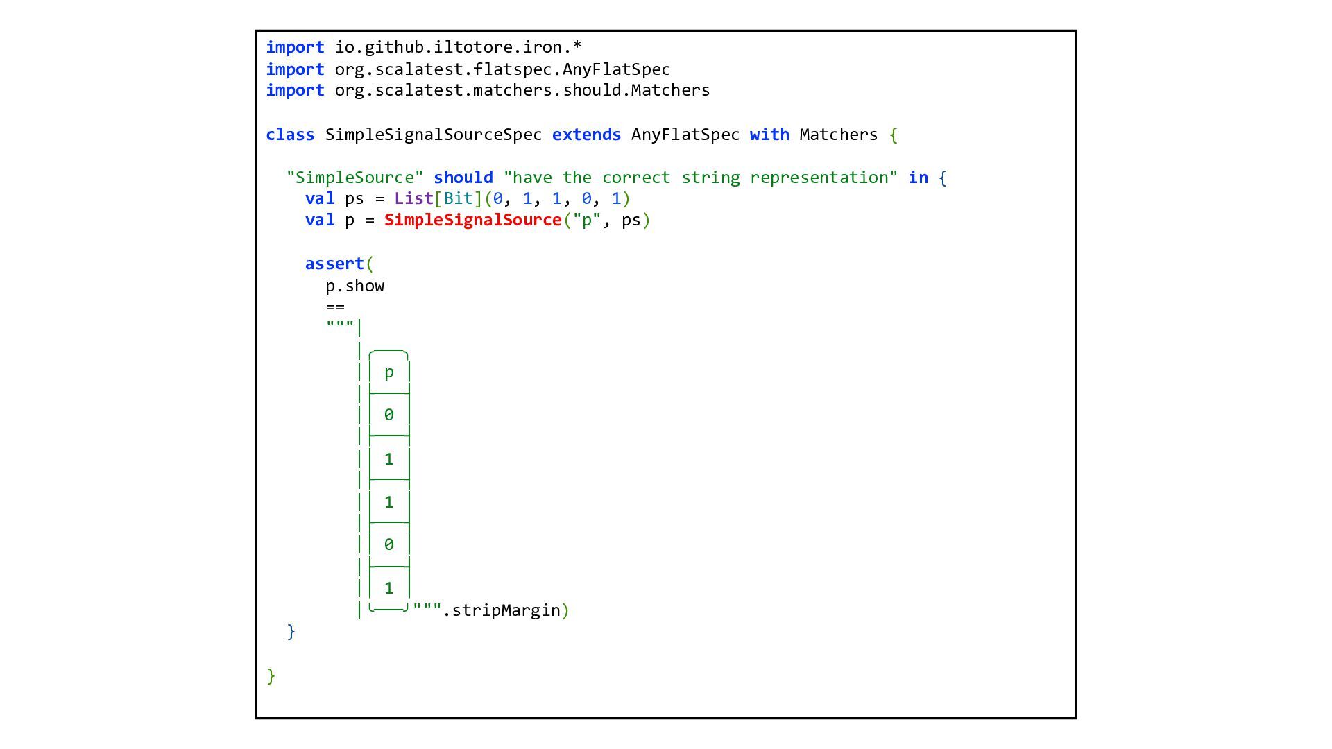
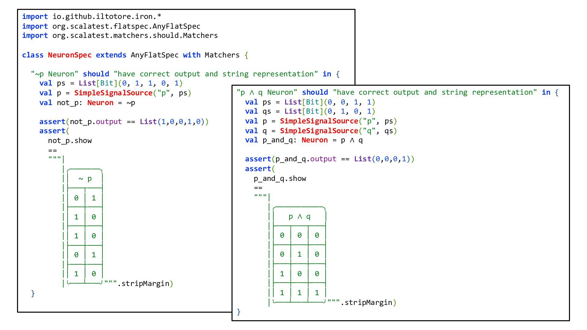
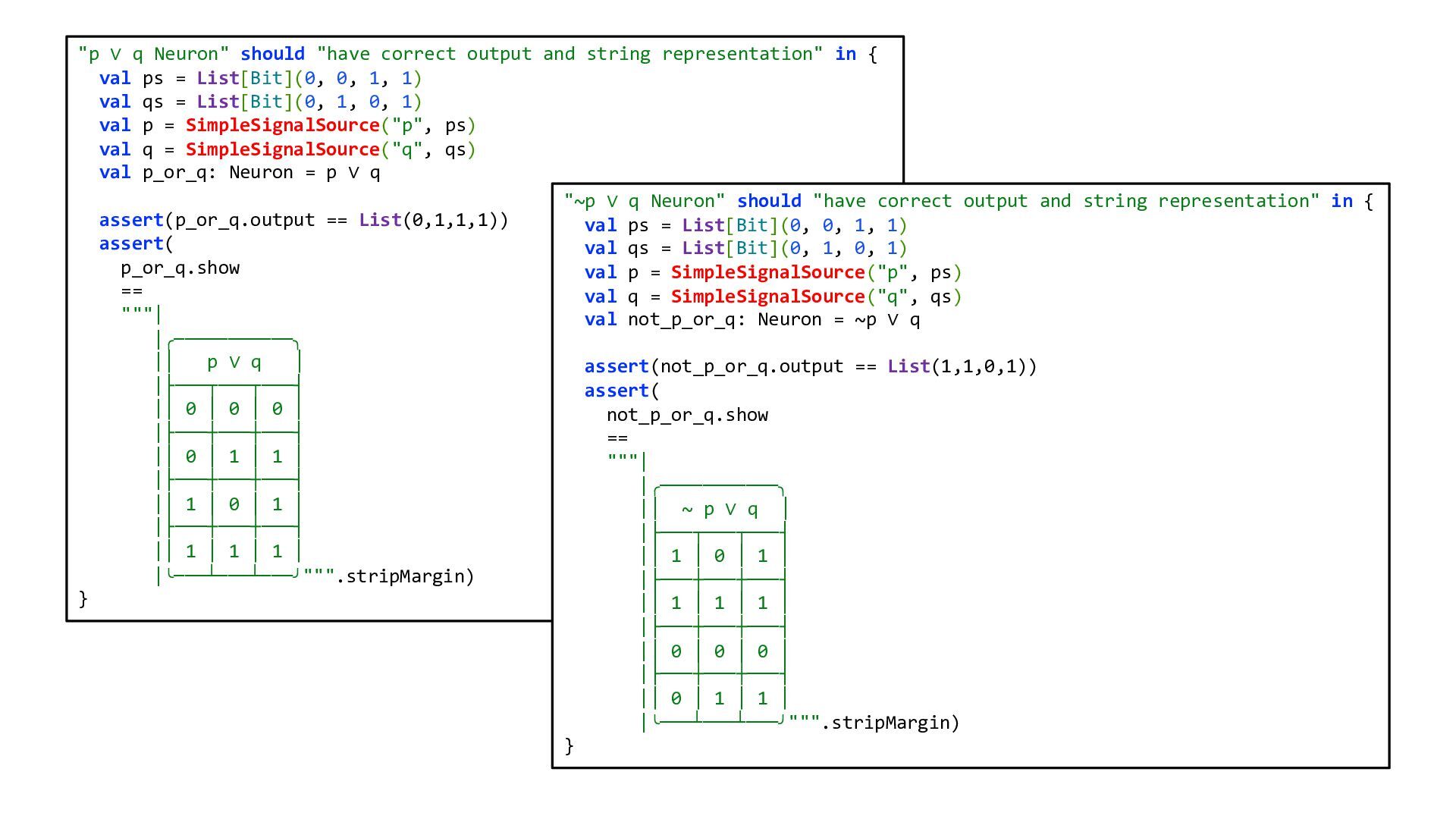
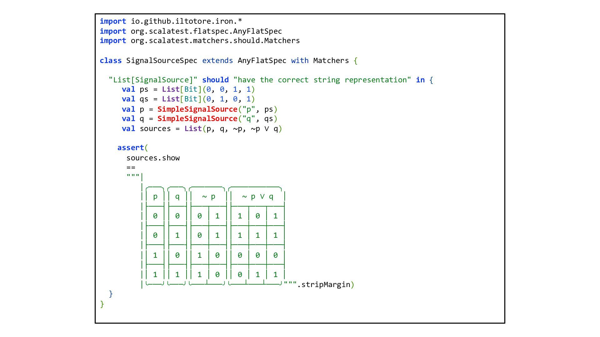
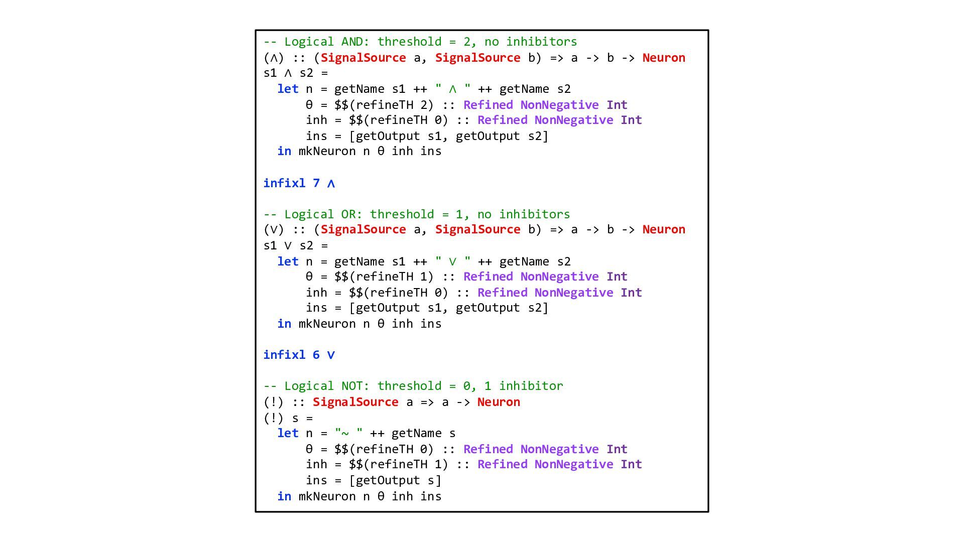
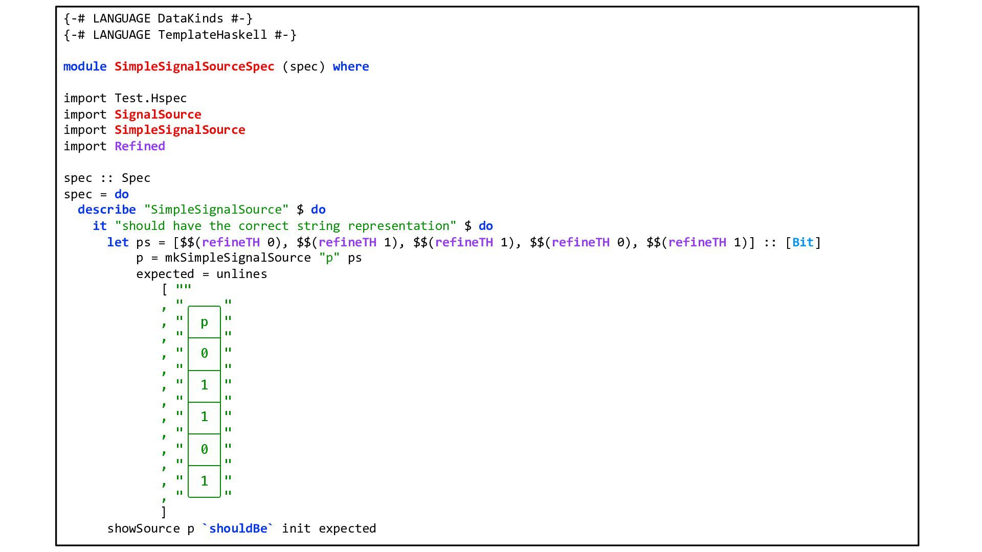
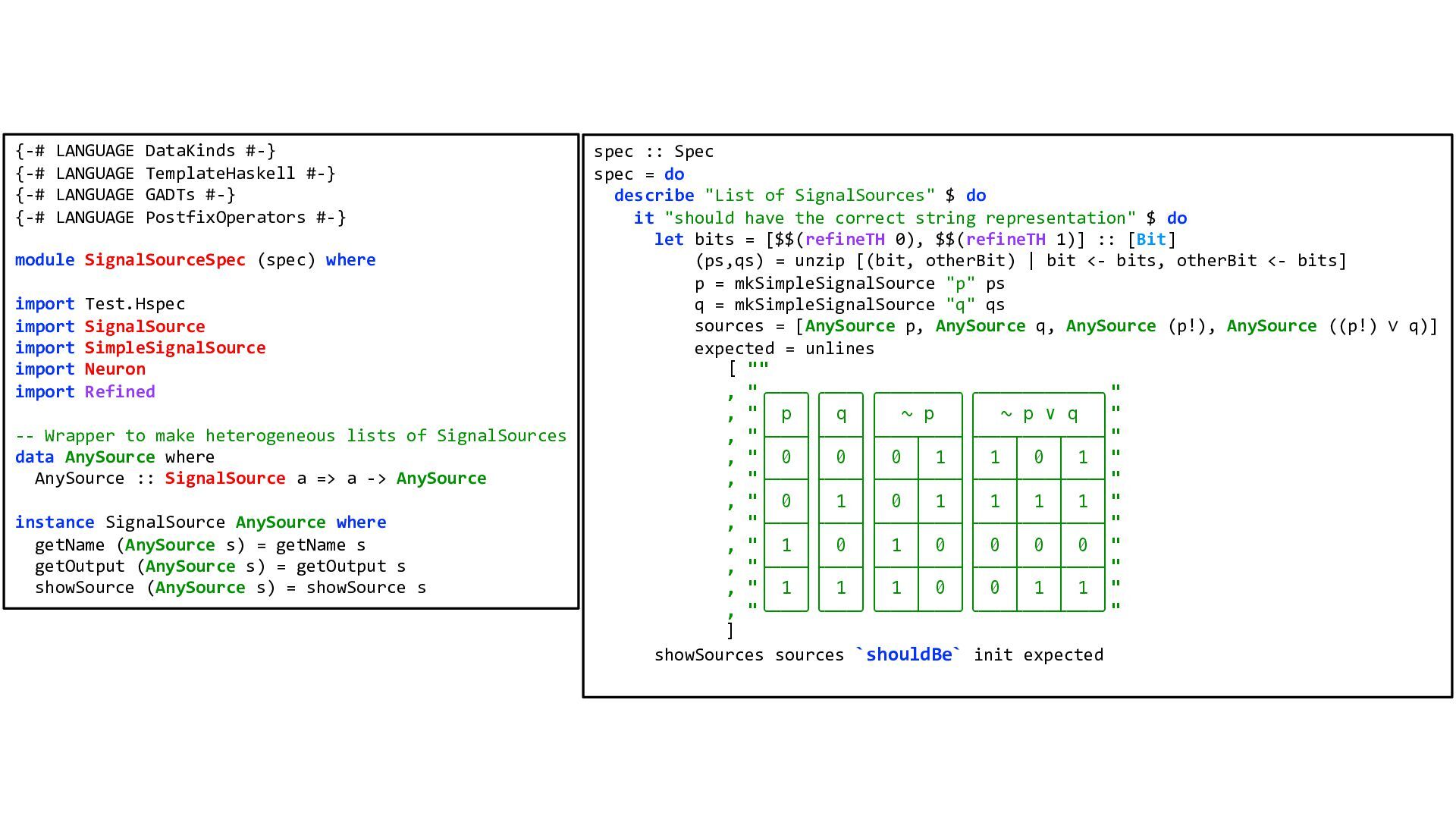
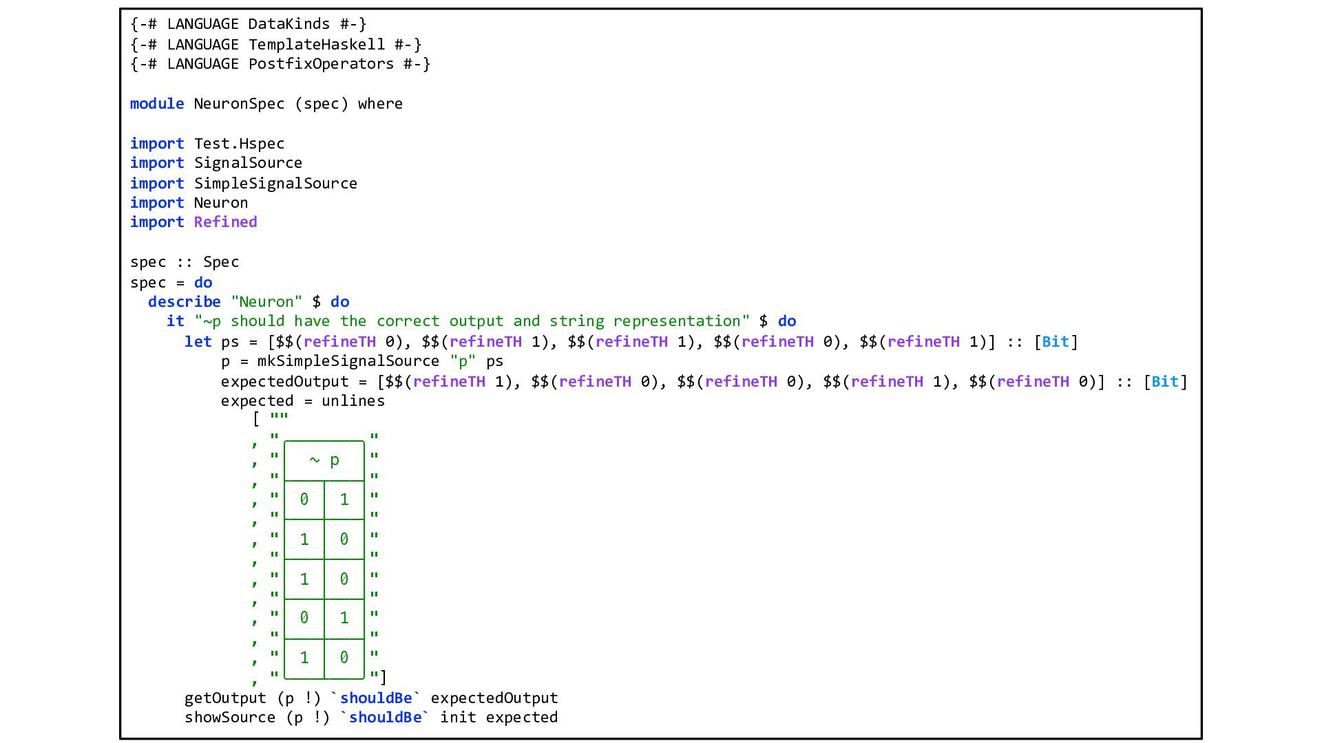
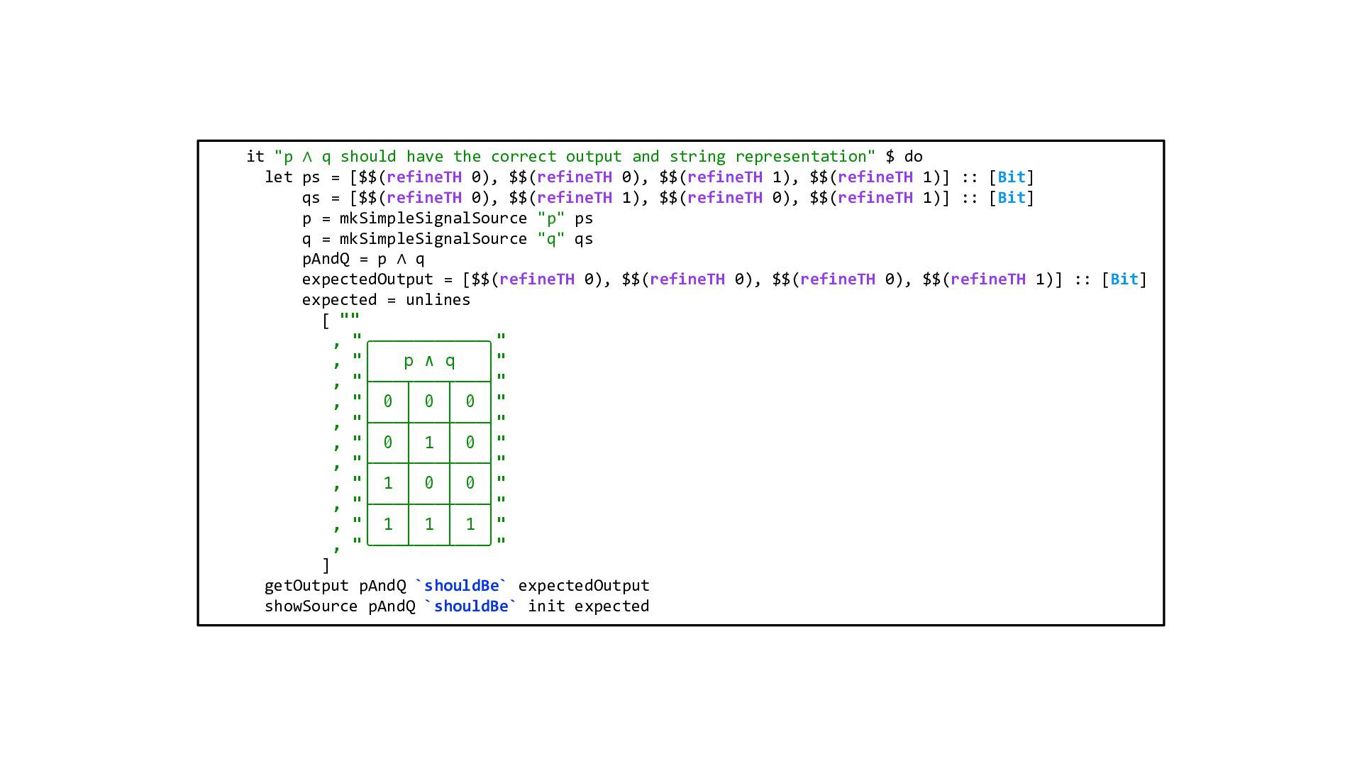
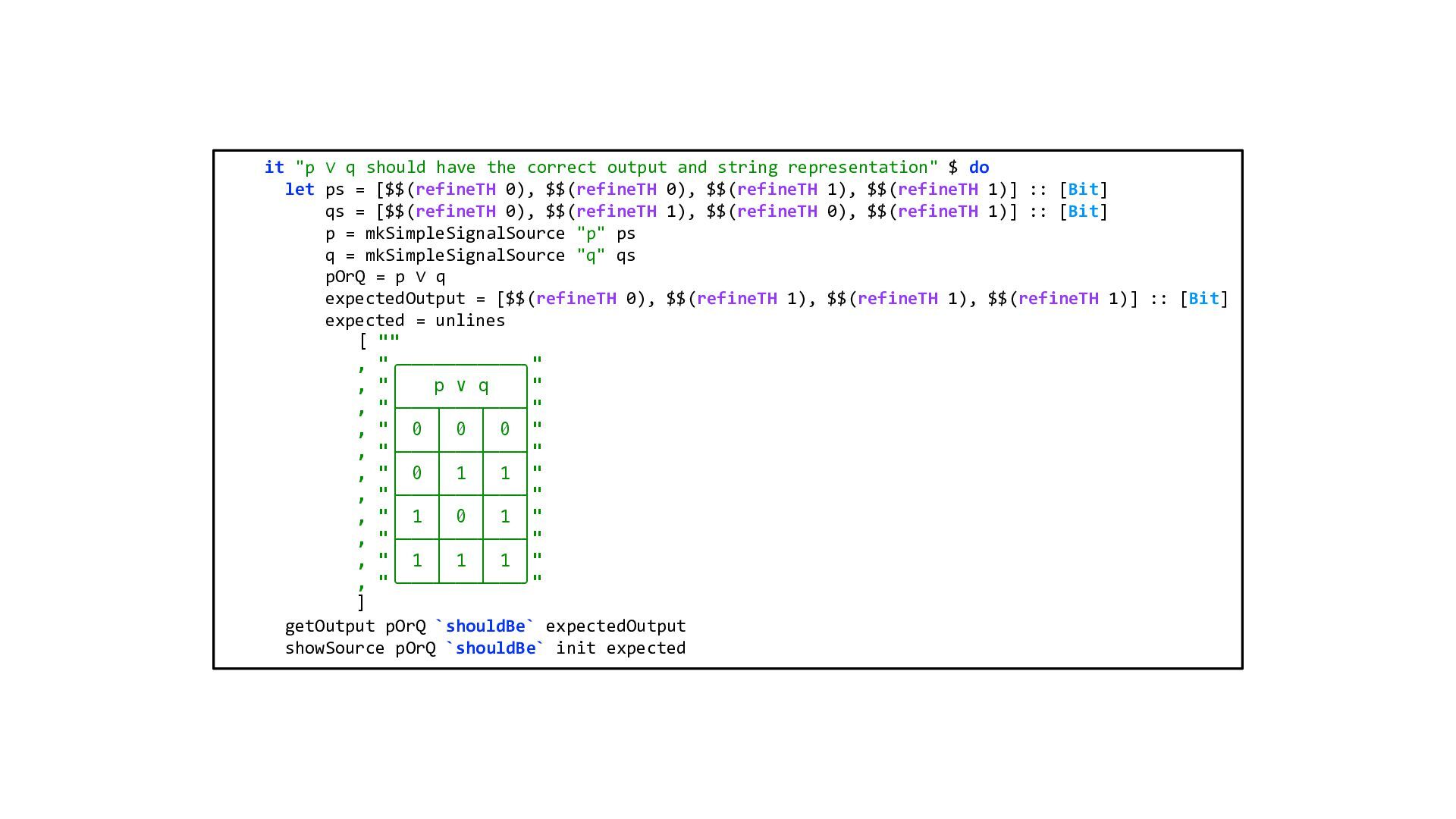
* Create simple MCP Neurons implementing key logical operators
* Combine such Neurons to create small neural nets implementing more complex logical propositions.

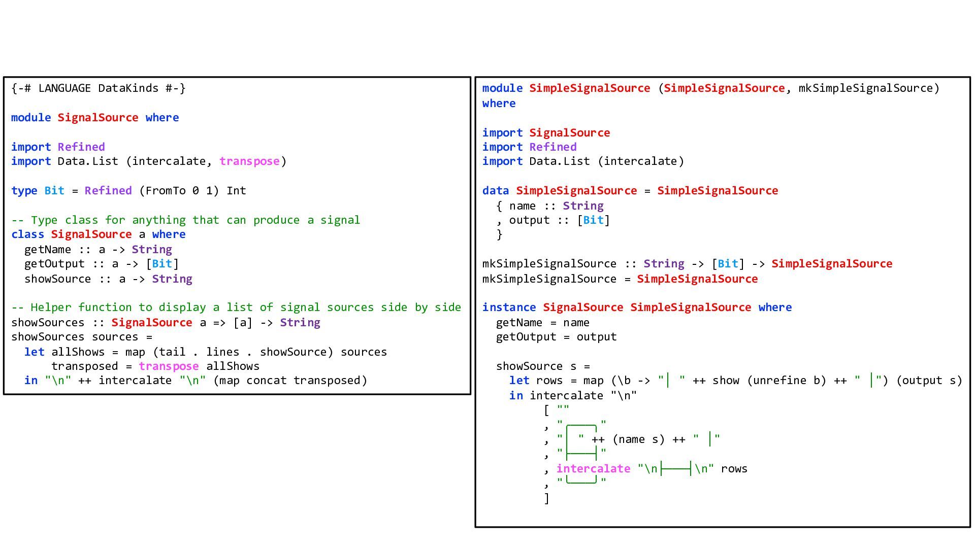
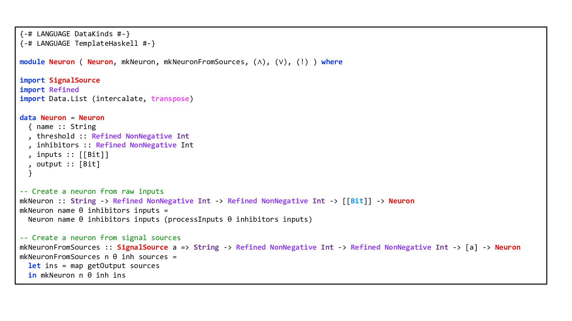
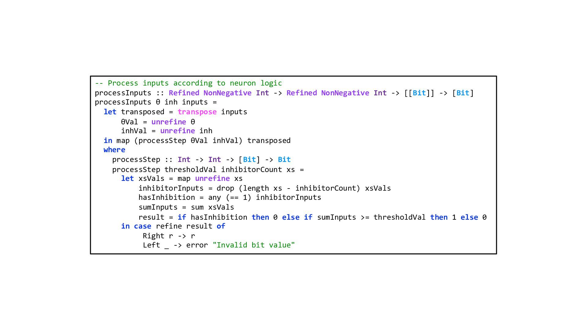
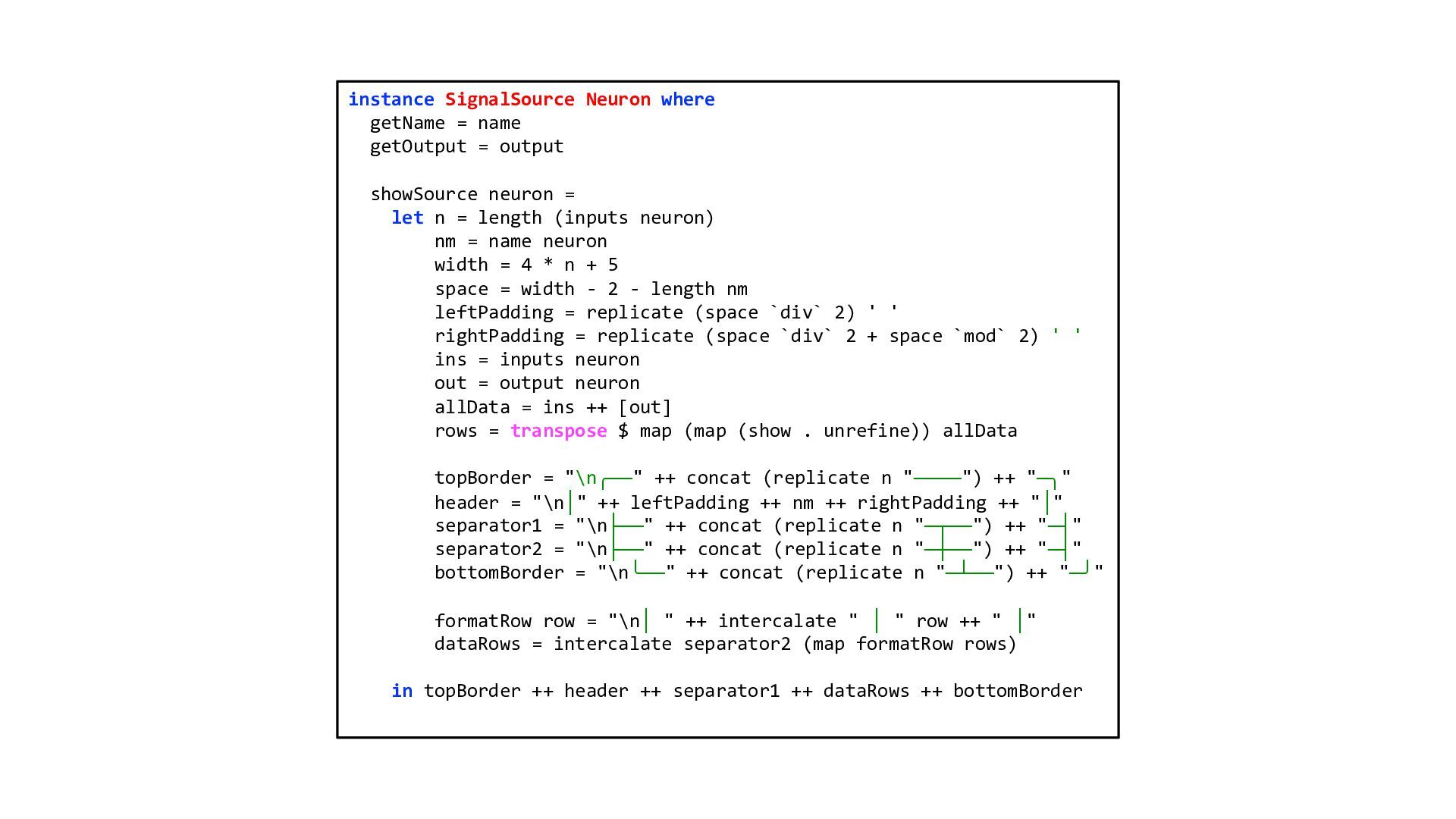
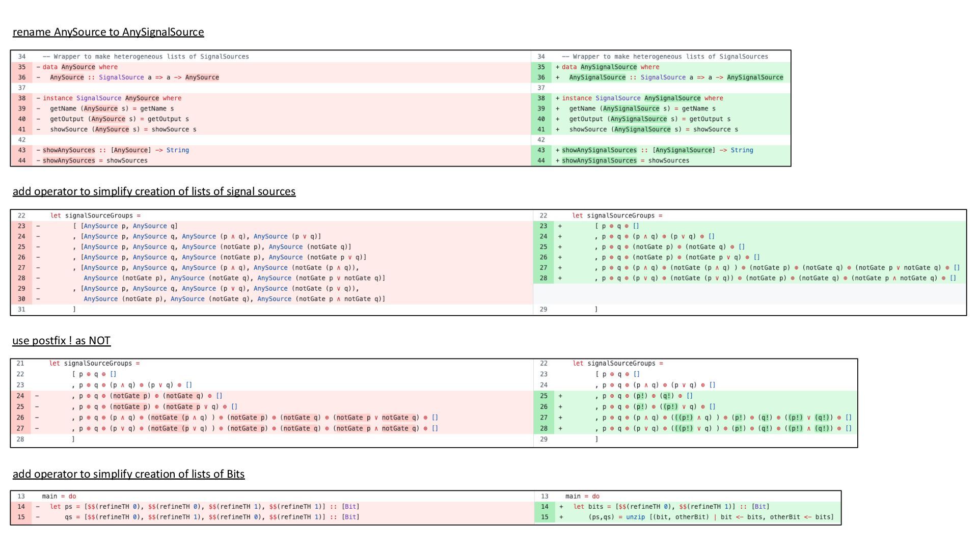
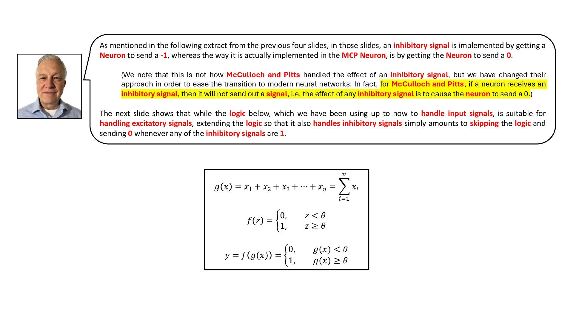
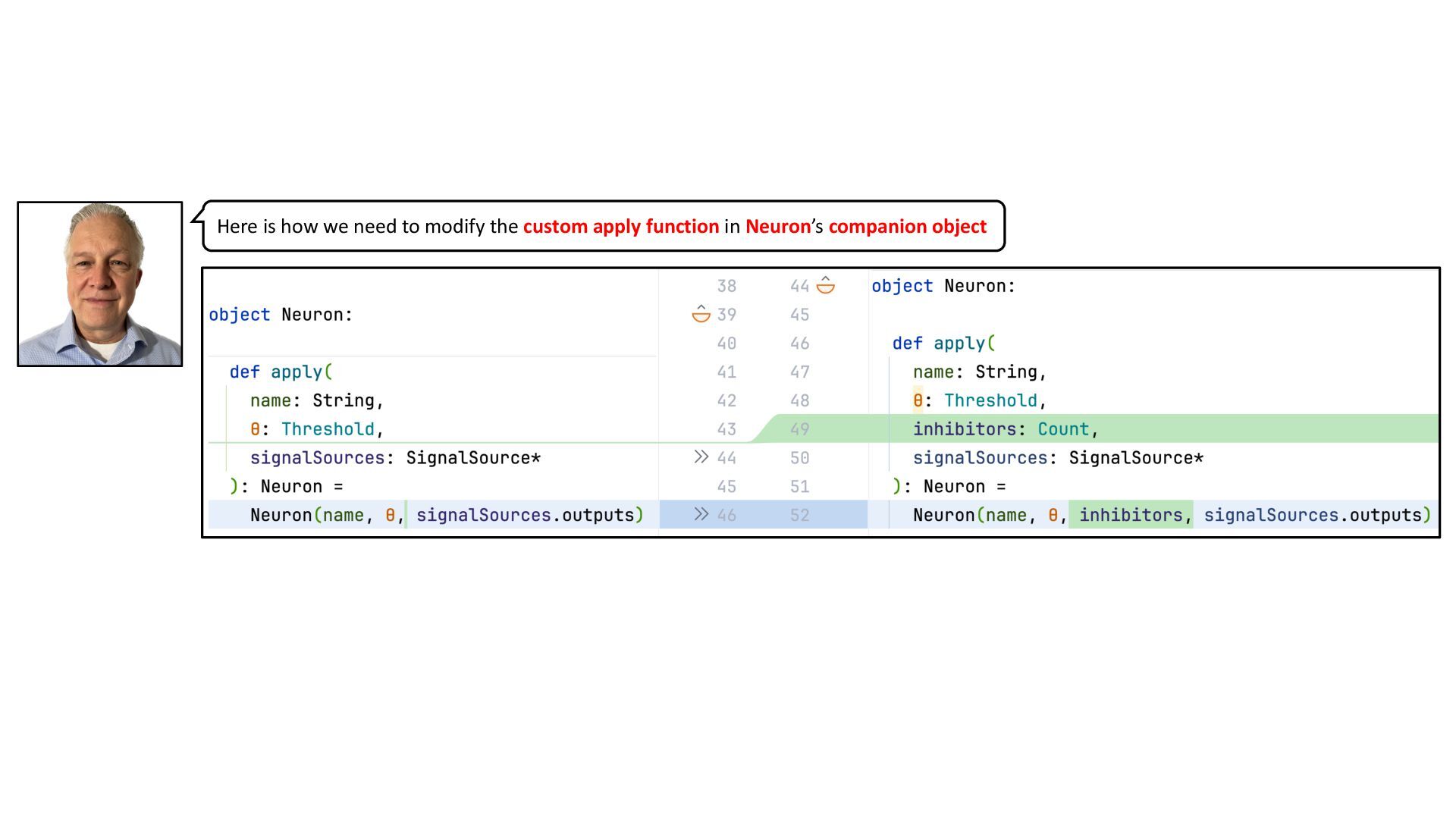
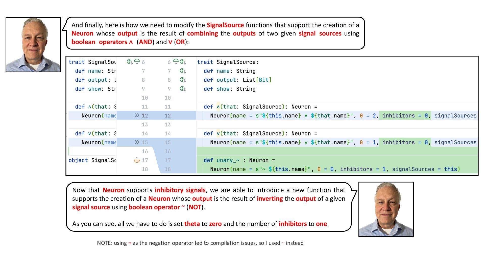
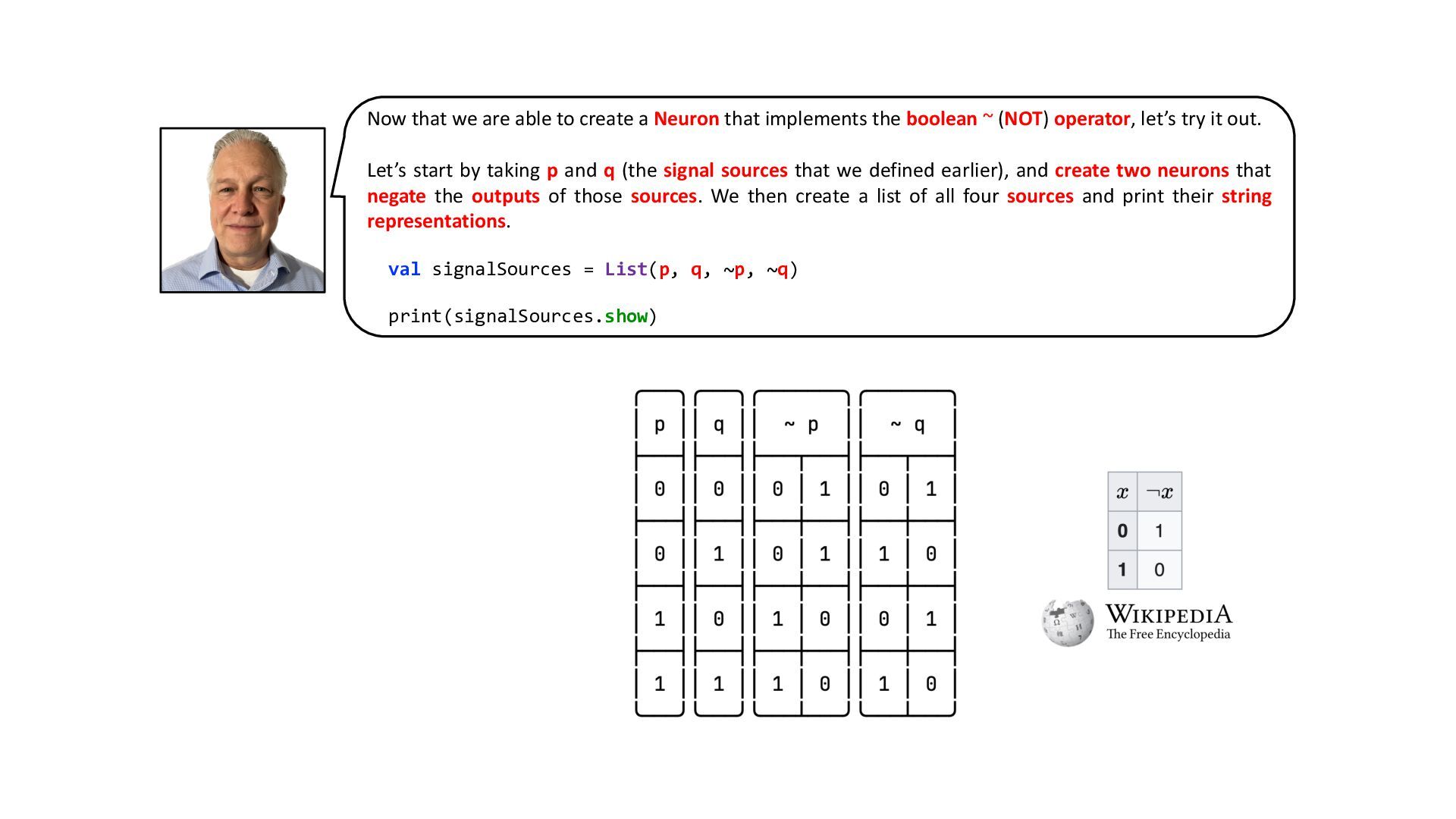
Keywords: "Artificial Intelligence","Neuron","Neurode","MCP Neuron", "Artificial Neuron", "Neural Net", "Warren McCulloch", "Walter Pitts", "propositional logic", "boolean logic", "AND", "OR", "NOT", "excitatory signal", "inhibitory signal", "Scala"

Transcript

1. AI Concepts MCP Neurons through the writings of Anil Ananthaswamy and Dr. Michael Marsall (part 1 of a series) Anil Ananthaswamy Dr. Michael Marsalli @philip_schwarz slides by https://fpilluminated.org/ code edition
2. In this first deck in the series on Artificial Intelligence concepts we look at the MCP Neuron. After learning its formal mathematical definition, we write a program that allows us to • create simple MCP Neurons implementing key logical operators • combine such Neurons to create small neural nets implementing more complex logical propositions While the code in this edition of the deck is in Scala, the above program is very simple, and so is easily understood by programmers familiar with any functional programming language. Depending on demand, future editions in other languages are very likely, so look out for them. @philip_schwarz
3. While in part 1 of this series we are going to cover the concept of the MCP Neuron, we are doing so partly because the paper that introduced it forms the roots of the subsequent concept of the Perceptron, which we’ll cover in part 2. We’ll get started with the MCP Neuron right after the next two slides, which provide some context in the form of a minimal introduction to the Perceptron.
4. https://computerhistory.org/blog/chm-releases-alexnet-source-code/ Cornell University psychologist Frank Rosenblatt developed the Perceptron Mark I, an electronic neural network designed to recognize images—like letters of the alphabet. He introduced it to the public in 1958.
5. According to Rosenblatt, the perceptron would be the “first device to think as the human brain” and such machines might even be sent to other planets as “mechanical space explorers.” None of this happened. The perceptron never lived up to the hype. Nonetheless, Rosenblatt’s work was seminal. Almost every lecturer on artificial intelligence (AI) today will harken back to the perceptron. And that’s justified. This moment in history—the arrival of large language models (LLMs) such as ChatGPT and its ilk and our response to it—which some have likened to what it must have felt like in the 1910s and ’20s, when physicists were confronted with the craziness of quantum mechanics, has its roots in research initiated by Rosenblatt. Anil Ananthaswamy @anilananth Academic interests Perceptron Rosenblatt is best known for the Perceptron, an electronic device which was constructed in accordance with biological principles and showed an ability to learn. Rosenblatt's perceptrons were initially simulated on an IBM 704 computer at Cornell Aeronautical Laboratory in 1957. When a triangle was held before the perceptron's eye, it would pick up the image and convey it along a random succession of lines to the response units, where the image was registered. Frank Rosenblatt
6. The next slide begins to introduce Warren McCulloch, Walter Pitts, and the paper in which they wrote about the MCP Neuron.
7. Chapter 1 - Desperately Seeking Patterns … THE FIRST ARTIFICIAL NEURON The perceptron’s roots lie in a 1943 paper by an unlikely combination of a philosophically minded neuroscientist in his mid- forties and a homeless teenager. Warren McCulloch was an American neurophysiologist trained in philosophy, psychology, and medicine. During the 1930s, he worked on neuroanatomy, creating maps of the connectivity of parts of monkey brains. While doing so, he also obsessed over the “logic of the brain.” By then, the work of mathematicians and philosophers like Alan Turing, Alfred North Whitehead, and Bertrand Russell was suggesting a deep connection between computation and logic. The statement “If P is true AND Q is true, then S is true” is an example of a logical proposition. The assertion was that all computation could be reduced to such logic. Given this way of thinking about computation, the question bothering McCulloch was this: If the brain is a computational device, as many think it is, how does it implement such logic? With these questions in mind, McCulloch moved in 1941 from Yale University to the University of Illinois, where he met a prodigiously talented teenager named Walter Pitts. The youngster, already an accomplished logician (“a protégé of the eminent mathematical logician Rudolf Carnap”), was attending seminars run by Ukrainian mathematical physicist Nicolas Rashevsky in Chicago. Pitts, however, was a “mixed-up adolescent, essentially a runaway from a family that could not appreciate his genius.” Dr. Michael Marsalli In 1943 Warren S. McCulloch, a neuroscientist, and Walter Pitts, a logician, published "A logical calculus of the ideas immanent in nervous activity" in the Bulletin of Mathematical Biophysics 5:115-133. Anil Ananthaswamy @anilananth
8. The next three slides show 1. Photos of Warren McCulloch and Walter Pitts 2. The abstract of their paper 3. The paper’s diagrams of sample nervous nets, the first four being fundamental building blocks: a) precession (identity) b) disjunction (OR) c) conjunction (AND) d) negated conjunction 4. Temporal Propositional Expressions (TPEs) corresponding to the diagrams As for the diagrams and TPEs, they are only there to provide you with a flavour of what you can expect if you decide to take a look at the paper. You don’t need to make any sense of them in order to follow this deck.
9. Warren McCulloch Walter Pitts
10. https://www.cs.cmu.edu/~epxing/Class/10715/reading/McCulloch.and.Pitts.pdf
12. The next slide continues to introduce Warren McCulloch, Walter Pitts, and the paper in which they wrote about the MCP Neuron.
13. Dr. Michael Marsalli https://www.researchgate.net / profile/Michael-Marsalli-2 https://youtu.be/DiteeU29dA0 McCulloch-Pitts Neurons: Introductory Level A computer model of the neuron In 1943 Warren S. McCulloch, a neuroscientist, and Walter Pitts, a logician, published "A logical calculus of the ideas immanent in nervous activity" in the Bulletin of Mathematical Biophysics 5:115-133. In this paper McCulloch and Pitts tried to understand how the brain could produce highly complex patterns by using many basic cells that are connected together. These basic brain cells are called neurons, and McCulloch and Pitts gave a highly simplified model of a neuron in their paper. The McCulloch and Pitts model of a neuron, which we will call an MCP neuron for short, has been very important in computer science. In fact, you can buy an MCP neuron at most electronic stores, but they are called "threshold logic units." A group of MCP neurons that are connected together is called an artificial neural network. In a sense, the brain is a very large neural network. It has billions of neurons, and each neuron is connected to thousands of other neurons. McCulloch and Pitts showed how to encode any logical proposition by an appropriate network of MCP neurons. And so in theory anything that can be done with a computer can also be done with a network of MCP neurons. McCulloch and Pitts also showed that every network of MCP neurons encodes some logical proposition. So if the brain were a neural network, then it would encode some complicated computer program. But the MCP neuron is not a real neuron; it's only a highly simplified model. We must be very careful in drawing conclusions about real neurons based on properties of MCP neurons. https://mind.ilstu.edu /curriculum/mcp_neurons /mcp_neuron1.html
14. With those introductory slides out of the way, let’s get to the meat of this deck. The next three slides provide a formal mathematical definition of the simple neurode (MCP Neuron). After that, we turn to implementing the MCP Neuron in Scala.
15. Dendrites Cell body Axon Axon Terminals Chapter 1 - Desperately Seeking Patterns … THE FIRST ARTIFICIAL NEURON …Taffy’s drawings would later illustrate McCulloch and Pitts’s 1943 paper, “A Logical Calculus of the Ideas Immanent in Nervous Activity.” In that work, McCulloch and Pitts proposed a simple model of a biological neuron. First, here’s an illustration of a generic biological neuron: The neuron’s cell body receives inputs via its treelike projections, called dendrites. The cell body performs some computation on these inputs. Then, based on the results of that computation, it may send an electrical signal spiking along another, longer projection, called the axon. That signal travels along the axon and reaches its branching terminals, where it’s communicated to the dendrites of neighboring neurons. And so it goes. Neurons interconnected in this manner form a biological neural network. McCulloch and Pitts turned this into a simple computational model, an artificial neuron. They showed how by using one such artificial neuron, or neurode (for “neuron” + “node”), one could implement certain basic Boolean logical operations such as AND, OR, NOT, and so on, which are the building blocks of digital computation. (For some Boolean operations, such as exclusive-OR, or XOR, you need more than one neurode, but more on this later.) Anil Ananthaswamy @anilananth NOTE: the Neuron image differs in unimportant ways from the one in the book
16. What follows is an image of a single neurode. (Ignore the “𝑔” and “𝑓” inside the neuron for now; we’ll come to those in a moment.) In this simple version of the McCulloch-Pitts model, 𝑥1 and 𝑥2 can be either 0 or 1. In formal notation, we can say: 𝑥1 , 𝑥2 ∈ {0, 1} That should be read as 𝑥1 is an element of the set {0, 1} and 𝑥2 is an element of the set {0, 1}; 𝑥1 and 𝑥2 can take on only values 0 or 1 and nothing else. The neurode’s output 𝑦 is calculated by first summing the inputs and then checking to see if that sum is greater than or equal to some threshold, theta (𝜃). If so, 𝑦 equals 1; if not, 𝑦 equals 0. 𝑠𝑢𝑚 = 𝑥1 + 𝑥2 𝐼𝑓 𝑠𝑢𝑚 ≥ 𝜃: 𝑦 = 1 𝐸𝑙𝑠𝑒: 𝑦 = 0 𝑔 𝑓 𝑥1 𝑥2 𝑦 Anil Ananthaswamy @anilananth NOTE: to help keep text less cluttered, the book dispenses with subscripts, whereas in this deck, they have been 'restored'.
17. Generalizing this to an arbitrary sequence of inputs, 𝑥1 , 𝑥2 , 𝑥3 , … 𝑥𝑛 , one can write down the formal mathematical description of the simple neurode. First, we define the function 𝑔(𝑥)—read that as “𝑔 of 𝑥,” where 𝑥 here is the set of inputs (𝑥1 , 𝑥2 , 𝑥3 , … 𝑥𝑛 )— which sums up the inputs. Then we define the function 𝑓(𝑔(𝑥))—again, read that as “𝑓 of 𝑔 of 𝑥”—which takes the summation and performs the thresholding to generate the output, 𝑦 : It is zero if 𝑔(𝑥) is less than some 𝜃 and 1 if 𝑔(𝑥) is greater than or equal to 𝜃. 𝑔 𝑥 = 𝑥1 + 𝑥2 + 𝑥3 + ⋯ + 𝑥𝑛 = < !"# $ 𝑥𝑖 𝑓 𝑧 = > 0, 𝑧 < 𝜃 1, 𝑧 ≥ 𝜃 𝑦 = 𝑓 𝑔(𝑥) = > 0, 𝑔(𝑥) < 𝜃 1, 𝑔(𝑥) ≥ 𝜃 With one artificial neuron as described, we can design some of the basic Boolean logic gates (AND & OR, for example). In an AND logic gate, the output 𝑦 should be 1 if both 𝑥1 and 𝑥2 are equal to 1; otherwise, the output should be 0. In this case, 𝜃 = 2 does the trick. Now, the output 𝑦 will be 1 only when 𝑥1 and 𝑥2 are both 1 (only then will 𝑥1 + 𝑥2 be greater than or equal to 2). You can play with the value of 𝜃 to design the other logic gates. For example, in an OR gate, the output should be 1 if either 𝑥1 or 𝑥2 is 1; otherwise, the output should be 0. What should 𝜃 be? Anil Ananthaswamy @anilananth
18. Let’s have a go at implementing the MCP Neuron. The first thing we need is an abstraction for the sources of the binary signals that are to be the inputs consumed by Neurons. trait SignalSource: def name: String def output: List[Bit] def show: String The name is used to identify the source of the signal. As for the signal emitted by the source, we can obtain it by asking for the source’s output. We can also ask the source to show us a textual representation of the source’s name and output. The output consists of a sequence of values of type Bit, whose possible values are integers 0 and 1. We decided to define the Bit type using Iron, a lightweight library for refined types in Scala 3: import io.github.iltotore.iron.* import io.github.iltotore.iron.constraint.numeric.Interval.Closed type Bit = Int :| Closed[0, 1] The way we constrain the permitted values to be either 0 or 1 is by specifying them to be the integers in the closed range from 0 to 1, i.e. a range inclusive of its bounds 0 and 1.
19. The first type of signal source is simple and looks like this: case class SimpleSignalSource( name: String, output: List[Bit] ) extends SignalSource : override def show: String = List( "\n╭───╮", "\n│ " + name + " │", output.map("\n│ "+_+" │").mkString( "\n├───┤", "\n├───┤", "\n╰───╯" ) ).mkString If we define two short lists of bits, we can then define two simple signal sources whose outputs are the two lists val ( ps , qs ) : (List[Bit], List[Bit]) = List[(Bit,Bit)]( ( 0 , 0 ), ( 0 , 1 ), ( 1 , 0 ), ( 1 , 1 ) ).unzip val p = SimpleSignalSource("p", ps) val q = SimpleSignalSource("q", qs) trait SignalSource: def name: String def output: List[Bit] def show: String
20. Let’s ask signal source p for its string representation and print it to the console: print(p.show) We’ll soon be showing more than one signal source, so let’s add to the SignalSource companion object a show extension function which, given multiple sources, returns a string that aggregates their string representations so that they are shown next to each other: extension (signalSources: List[SignalSource]) def show: String = signalSources .map(_.show.split("\n").toList.tail) .transpose .map(_.mkString) .mkString("\n","\n","") Let’s try it out val signalSources = List(p, q) print(signalSources.show)
21. What about Neurons? While a Neuron consumes the outputs of one or more signal sources, it also produces an output that is a signal, so a Neuron is itself a signal source. Let’s introduce a SignalSource that is a Neuron: case class Neuron( name: String, θ: Threshold, inputs: List[List[Bit]] ) extends SignalSource: val output: List[Bit] = ??? override def show: String = ??? In addition to the name, output, and show function of a signal source, a Neuron has a threshold theta, and a list of inputs which are the binary signals that are the outputs of signal sources. As for the Threshold type, it is either zero or a positive integer, import io.github.iltotore.iron.* import io.github.iltotore.iron.constraint.numeric.Positive0 type Threshold = Int :| Positive0 trait SignalSource: def name: String def output: List[Bit] def show: String
22. Now let’s implement the logic that produces the Neuron’s output val output: List[Bit] = process(inputs) private def process(inputs: List[List[Bit]]): List[Bit] = inputs.transpose.map { xs => f(g(xs)) } private def g(xs: List[Bit]): Int = xs.sum private def f(z: Int): Bit = if z < θ then 0 else 1 The process function’s first step is to take the Neuron’s inputs, i.e. a list of 𝑛 SignalSource outputs with the 𝑖𝑡ℎ output being List(𝑥𝑖1 , 𝑥𝑖2 , … , 𝑥𝑖𝑚 ), and transpose it into a list of 𝑚 parameter lists with the 𝑖𝑡ℎ parameter list being List(𝑥1𝑖 , 𝑥2𝑖 , … , 𝑥𝑛𝑖 ). The process function’s second step is to map each parameter list List(𝑥1𝑖 , 𝑥2𝑖 , … , 𝑥𝑛𝑖 ), referred to as 𝑥, to 𝑓 𝑔(𝑥) , referred to as 𝑦𝑖 , thereby producing output List(𝑦1 , 𝑦2 , … , 𝑦𝑚 ). 𝑔 𝑥 = 𝑥1 + 𝑥2 + 𝑥3 + ⋯ + 𝑥𝑛 = & )*+ , 𝑥𝑖 𝑓 𝑧 = ) 0, 𝑧 < 𝜃 1, 𝑧 ≥ 𝜃 𝑦 = 𝑓 𝑔(𝑥) = ) 0, 𝑔(𝑥) < 𝜃 1, 𝑔(𝑥) ≥ 𝜃 List(List 𝑥11 , 𝑥12 , … , 𝑥1𝑚 , List 𝑥21 , 𝑥22 , … , 𝑥2𝑚 , … , List 𝑥𝑛1 , 𝑥𝑛2 , … , 𝑥𝑛𝑚 ) ⇓ 𝑠𝑡𝑒𝑝 1 − 𝑡𝑟𝑎𝑛𝑠𝑝𝑜𝑠𝑒 List(List 𝑥11 , 𝑥21 , … , 𝑥𝑛1 , List 𝑥12 , 𝑥22 , … , 𝑥𝑛2 … , List 𝑥1𝑚 , 𝑥2𝑚 , … , 𝑥𝑛𝑚 )) ⇓ 𝑠𝑡𝑒𝑝2 − 𝑓𝑜𝑟 𝑖 𝑖𝑛 1. . 𝑚: 𝑥 = 𝑥1𝑖 , 𝑥2𝑖 , … , 𝑥𝑛𝑖 ; 𝑦𝑖 = 𝑓 𝑔 𝑥 List(y1 , y2 , … , ym )
23. As an example of the transposition carried out by the process function… private def process(inputs: List[List[Bit]]): List[Bit] = inputs.transpose.map { xs => f(g(xs)) } …if the inputs parameter consists of the outputs of p and q (the two signal sources that we defined earlier)… List[List[Bit]](p.output, q.output) … then the transposition looks like this: // Neuron inputs in the form of SignalSource outputs, i.e. List[List[Bit]](p.output, q.output) List( List(0, 0, 1, 1), // p at times t0, t1, t2 and t3 List(0, 1, 0, 1) // q at times t0, t1, t2 and t3 ) Transposition // Neuron inputs in the form of (x1, x2) pairs List( List(0, 0), // x1 and x2 at time t0 List(0, 1), // x1 and x2 at time t1 List(1, 0), // x1 and x2 at time t2 List(1, 1) // x1 and x2 at time t3 )
24. There are three tasks left to finish implementing our first version of the Neuron. The first task is implementing the show function. Feel free to ignore the following code for now, and consider coming back to it once you have seen it in action, if you decide that you are be interested in how it works. override def show: String = val n = inputs.size val width = 4 * n + 5 val space = width - 2 - name.size val leftPadding = " " * (space / 2) val rightPadding = " " * (space / 2 + space % 2) List( "\n╭──" + "────" * n + "─╮", "\n│" + leftPadding + name + rightPadding + "│", (inputs ++ List(output)).transpose.map(_.mkString( "\n│ ", " │ ", " │")).mkString( "\n├──" + "─┬──" * n + "─┤", "\n├──" + "─┼──" * n + "─┤", "\n╰──" + "─┴──" * n + "─╯") ).mkString By the way, the above code is subject to the limitation that its results are only aesthetically correct in the case of Neurons with suitably short names, which is what we’ll be using in upcoming examples.
25. The second task left is to provide the Neuron with a custom apply function that makes it more convenient to supply the Neuron’s input signals, in that rather than having to take the outputs of desired signal sources and supply a list of such outputs, we can just supply the signal sources as if they were parameters of the apply function. As you can see below, the new custom apply function relies on a new subordinate outputs extension function in the SignalSource companion object. Again, feel free to ignore the following code for now. object Neuron: def apply( name: String, θ: Threshold, signalSources: SignalSource* ): Neuron = Neuron(name, θ, signalSources.outputs) object SignalSource: extension (signalSources: Seq[SignalSource]) def outputs: List[List[Bit]] = signalSources.toList.map(_.output)
26. The third and final task left for implementing the first version of the Neuron is to provide functions to support the creation of a Neuron whose output is the result of combining the outputs of two given signal sources using boolean operators ∧ (AND) and ∨ (OR): trait SignalSource: def name: String def output: List[Bit] def show: String def ∧(that: SignalSource): Neuron = Neuron(name = s"${this.name} ∧ ${that.name}", θ = 2, signalSources = this, that) def ∨(that: SignalSource): Neuron = Neuron(name = s"${this.name} ∨ ${that.name}", θ = 1, signalSources = this, that) The name of the created Neuron indicates that its output is the ANDing or the ORing of its inputs. As for suitable theta values, while we learned earlier that “𝜃 = 2 does the trick” for AND, the question of what works for OR was left as an exercise, and the answer turns out to be 𝜃 = 1.
27. It is finally time to create a couple of sample Neurons, ask for their string representations, and print the latter to the console. Let’s take p and q (the two signal sources that we defined earlier), and create two neurons, one that ANDs the outputs of the two sources, and one that ORs them. We can then create a list of all four signal sources and print their string representations. val signalSources = List(p, q, p ∧ q, p ∨ q) print(signalSources.show) It works nicely! In this case it seems a bit superfluous to explicitly display signal sources p and q because their outputs already get implicitly displayed as a result of displaying p ∨ q and p ∧ q, but once examples get more complex, it can help to have all intermediate signal sources and neurons displayed.
28. Our Neuron examples p ∧ q and p ∨ q are abstract because so are their input signals p and q. If you could do with a less abstract example of a Neuron, the next four slides provide one involving a bird, a blueberry, a violet, a golf ball and a hot dog. Feel free to skip the example, but don’t be put off by the number of slides, as they make for light reading. The subsequent four slides are my visualisation of the example and can be understood even if you skip the previous four.
29. Some MCP neuron examples In order to understand MCP neurons, let's look at an example. Suppose there is a neuron in a bird's brain that has two receivers, which are connected somehow to the bird's eyes. If the bird sees a round object, a signal is sent to the first receiver. But if any other shape is seen, no signal is sent. So the first receiver is a roundness detector. If the bird sees a purple object, a signal is sent to the second receiver of the neuron. But if the object is any other color, then no signal is sent. So the second receiver is a purple detector. Notice that for either receiver there is a question that can be answered "yes" or "no," and a signal is only sent if the answer is "yes." The first receiver corresponds to the question "Is the object round?" The second receiver corresponds to the question "Is the object purple?" We would like to produce an MCP neuron that will tell the bird to eat a blueberry, but to avoid eating red berries or purple violets. In other words, we want the MCP neuron to send an "eat" signal if the object is both round and purple, but the MCP neuron will send no signal if the object is either not round or not purple, or neither round nor purple. So the bird will only eat an object if the MCP neuron sends a signal. If no signal is sent, then the bird will not eat the object. Dr. Michael Marsalli
30. Here is a table that summarizes how the MCP neuron would work in several cases. Notice that all the signals sent to the MCP neuron and the signal that it sends out are all "yes" or "no" signals. This "all or nothing" feature is one of the assumptions that McCulloch and Pitts made about the workings of a real neuron. They also assumed that somehow a real neuron "adds" the signals from all its receivers, and it decides whether to send out a "yes" or "no" signal based on the total of the signals it receives. If the total of the received signals is high enough, the neuron sends out a "yes" signal; otherwise, the neuron sends a "no" signal. In order to "add" the signals that the MCP neuron is receiving, we will use the number 1 for a "yes" and the number 0 for a "no." Object Purple? Round? Eat? Blueberry Yes Yes Yes Golf ball No Yes No Violet Yes No No Hot Dog No No No Table 1 Dr. Michael Marsalli
31. Then Table 1 will now look like this. Now we need a way to decide if the total of the received signals is "high enough." The way McCulloch and Pitts did this is to use a number they called a threshold. So what is a threshold, and how does it work? Every MCP neuron has its own threshold that it compares with the total of the signals it has received. If the total is bigger than or equal to the threshold, then the MCP neuron will send out a 1 (i.e. a "yes" signal). If the total is less than the threshold, then the MCP neuron will send out a 0 (i.e. a "no" signal). So the MCP neuron is answering the question "Is the sum of the signals I received greater than or equal to my threshold?” Object Purple? Round? Eat? Blueberry 1 1 1 Golf ball 0 1 0 Violet 1 0 0 Hot Dog 0 0 0 Table 2 Dr. Michael Marsalli
32. In order to see how this threshold idea works, let's suppose that we have an MCP neuron with two receivers connected to a bird's eyes. The one receiver is a roundness detector and the other is a purple detector, just as we had in the example above. Since we want the neuron to instruct the bird to eat blueberries but not golfball, violets or hotdogs we need a threshold high enough so that it requires that both of the two properties are present. Let's try a threshold of "2" and see if that doesn't work. If the bird sees a blueberry, then the purple detector sends a 1 and the roundness detector sends a 1. So our MCP neuron adds these signals to get a combined input of 1+1 =2. Now our MCP neuron takes this total input of 2 and compares it to its threshold of 2. Because the total input (= 2) is greater than or equal to the threshold (=2), the MCP neuron will send an output of 1 (which means, "EAT"). But how will the bird behave in the presence of a golfball? or in the presence of the other objects we've considered? To help you explore these questions and to aid your understanding of MCP neurons, we have a Flash animation of a bird deciding which objects to eat and which to avoid: https://mind.ilstu.edu/curriculum/mcp_neurons/mcp1.mp4. Dr. Michael Marsalli
33. 𝟎 𝑔 𝑓 𝑥1 𝑥2 𝑔 𝑥 = 𝑥1 + 𝑥2 + 𝑥3 + ⋯ + 𝑥𝑛 = & )*+ , 𝑥𝑖 𝑓 𝑧 = ) 0, 𝑧 < 𝜃 1, 𝑧 ≥ 𝜃 𝑦 = 𝑓 𝑔(𝑥) = ) 0, 𝑔(𝑥) < 𝜃 1, 𝑔(𝑥) ≥ 𝜃 Object Purple? Round? Eat? Blueberry 1 1 1 Golf ball 0 1 0 Violet 1 0 0 Hot Dog 0 0 0 𝟎 𝟎 Is the object round? Is the object purple? MCP neuron implementing an AND gate (𝜃 = 𝟐) 𝟎 + 𝟎 < 𝟐 𝟎 no 𝟏 yes signal on signal off eat?
34. 𝟎 𝑔 𝑓 𝑥1 𝑥2 𝑔 𝑥 = 𝑥1 + 𝑥2 + 𝑥3 + ⋯ + 𝑥𝑛 = & )*+ , 𝑥𝑖 𝑓 𝑧 = ) 0, 𝑧 < 𝜃 1, 𝑧 ≥ 𝜃 𝑦 = 𝑓 𝑔(𝑥) = ) 0, 𝑔(𝑥) < 𝜃 1, 𝑔(𝑥) ≥ 𝜃 Object Purple? Round? Eat? Blueberry 1 1 1 Golf ball 0 1 0 Violet 1 0 0 Hot Dog 0 0 0 Is the object purple? 𝟏 Is the object round? MCP neuron implementing an AND gate (𝜃 = 𝟐) 𝟎 + 𝟏 < 𝟐 𝟎 no 𝟏 yes signal on signal off eat? 𝟎
35. 𝟏 𝑔 𝑓 𝑥1 𝑥2 𝑔 𝑥 = 𝑥1 + 𝑥2 + 𝑥3 + ⋯ + 𝑥𝑛 = & )*+ , 𝑥𝑖 𝑓 𝑧 = ) 0, 𝑧 < 𝜃 1, 𝑧 ≥ 𝜃 𝑦 = 𝑓 𝑔(𝑥) = ) 0, 𝑔(𝑥) < 𝜃 1, 𝑔(𝑥) ≥ 𝜃 Object Purple? Round? Eat? Blueberry 1 1 1 Golf ball 0 1 0 Violet 1 0 0 Hot Dog 0 0 0 Is the object round? 𝟎 Is the object purple? MCP neuron implementing an AND gate (𝜃 = 𝟐) 𝟏 + 𝟎 < 𝟐 𝟎 no 𝟏 yes signal on signal off eat? 𝟎
36. 𝟏 𝑔 𝑓 𝑥1 𝑥2 MCP neuron implementing an AND gate (𝜃 = 𝟐) 𝑔 𝑥 = 𝑥1 + 𝑥2 + 𝑥3 + ⋯ + 𝑥𝑛 = & )*+ , 𝑥𝑖 𝑓 𝑧 = ) 0, 𝑧 < 𝜃 1, 𝑧 ≥ 𝜃 𝑦 = 𝑓 𝑔(𝑥) = ) 0, 𝑔(𝑥) < 𝜃 1, 𝑔(𝑥) ≥ 𝜃 Object Purple? Round? Eat? Blueberry 1 1 1 Golf ball 0 1 0 Violet 1 0 0 Hot Dog 0 0 0 eat? Is the object round? Is the object purple? 𝟏 𝟏 + 𝟏 ≥ 𝟐 𝟎 no 𝟏 yes signal on signal off 𝟏
37. For what it is worth, here is our original abstract example of an ANDing Neuron, repackaged as the Neuron used by a bird to determine if it is seeing a blueberry that it should eat: val purple = SimpleSignalSource("prpl", ps) val round = SimpleSignalSource("rnd", qs) val eat = purple ∧ round print(eat.show)
38. At some earlier point I said “There are three tasks left to finish implementing the first version of the Neuron”. The reason why I spoke of a first version is that there is one aspect of the MCP Neuron that we have not covered yet, and covering which will unveil a second, fuller version of the Neuron, and will lead us to modifying our Neuron implementation slightly. While the modification will be small, its benefits will be considerable. What is missing from our current notion of the Neuron is that up to now we have only considered input signals that are excitatory, whereas a Neuron can also receive input signals that are inhibitory. While the excerpt below merely introduces the subject of inhibitory signals, the following four slides explain it in full. The simple MCP model can be extended. You can increase the number of inputs. You can let inputs be “inhibitory,” meaning 𝑥1 or 𝑥2 can be multiplied by −1. If one of the inputs to the neurode is inhibitory and you set the threshold appropriately, then the neurode will always output a 1, regardless of the value of all the other inputs. This allows you to build more complex logic. As does interconnecting multiple neurodes such that the output of one neurode serves as the input to another. Anil Ananthaswamy @anilananth
39. Excitatory and inhibitory signals So far we have only considered signals coming from the bird's receivers that are added to the other signals coming from the other receivers. These types of signals are called excitatory because they excite the neuron toward possibly sending its own signal. The more excitatory signals a neuron receives, the closer the total will be to the neuron's threshold, and so the closer the neuron will be to sending its signal. So as the neuron receives more and more excitatory signals, it gets more and more excited, until the threshold is reached, and the neuron sends out its own signal. But there is another kind of signal that has the opposite effect on a neuron. These other signals are called inhibitory signals, and they have the effect of inhibiting the neuron from sending a signal. When a neuron receives an inhibitory signal, it becomes less excited, and so it takes more excitatory signals to reach the neuron's threshold. In effect, inhibitory signals subtract from the total of the excitatory signals, making the neuron more relaxed, and moving the neuron away from its threshold. MCP neurons with an inhibitory signal Now let's look at an example of an MCP neuron with an inhibitory signal. Let's consider a a particular type of bird, say a robin. Now the robin, which has red feathers on its breast, is safe around any red objects, including red creatures such as a cardinal. Suppose our robin's brain has a neuron with two receivers connected to the robin's eyes. Normally our robin will flee from any other creature it sees. If the robin sees another creature, an excitatory signal will be sent to the first receiver, which will try to cause the bird to flee. So the first receiver is a creature detector, and it excites our bird to fleeing. However, if the creature that the robin sees has red on it, an inhibitory signal will be sent to the second receiver, which will prevent the bird from fleeing. So the second receiver is a red detector, and it inhibits our bird from fleeing. Dr. Michael Marsalli
40. Suppose our robin sees a black cat. What would happen? The creature detector would send an excitatory signal to the neuron, and the red detector would send no signal. So the bird would flee. Suppose our robin sees a cardinal. The creature detector would send an excitatory signal to the neuron, and the red detector would send an inhibitory signal. So the bird would not flee, because the inhibitory signal would "cancel" the excitatory signal. Here is a table that summarizes how this MCP neuron with the excitatory and inhibitory signals would work in several cases. Now we'll see how these new ideas of excitatory and inhibitory signals work when the MCP neuron compares these signals to its threshold. As before, we'll use a 1 if an excitatory signal is sent, and a 0 if no excitatory signal is sent. But now we'll use a - 1 when an inhibitory signal is sent, and a 0 if no inhibitory signal is sent. Because we are using a -1 for an inhibitory signal, when we add an inhibitory signal to the total of all signals received, the effect of the inhibitory signal on the total is to subtract a 1. (Recall that adding a -1 is the same as subtracting a 1.) So when an MCP neuron computes the total effect of its signals, it will add a 1 to the total for each of the excitatory signals and add a -1 to the total for each of its inhibitory signals. If the total of excitatory signals and inhibitory signals is greater than or equal to the threshold, then the MCP neuron will send a 1. If the total of excitatory signals and inhibitory signals is less than the threshold, then the MCP neuron will send a 0. Object Creature? Red? Flee? Black Cat Yes No Yes Male Cardinal Yes Yes No Hot Dog No Yes No Table 4 Dr. Michael Marsalli
41. (We note that this is not how McCulloch and Pitts handled the effect of an inhibitory signal, but we have changed their approach in order to ease the transition to modern neural networks. In fact, for McCulloch and Pitts, if a neuron receives an inhibitory signal, then it will not send out a signal, i.e. the effect of any inhibitory signal is to cause the neuron to send a 0.) Let's look at an example. Suppose we have an MCP neuron connected to a creature detector that sends an excitatory signal and a red detector that sends an inhibitory signal. Let's also suppose the threshold is 1. We could have chosen another number for the threshold. Now for each object in Table 4, we can compute the total of the signals by adding a 1 for each excitatory signal and a -1 for each inhibitory signal. Then we compare the total to the threshold. If the robin sees a black cat, then the creature detector, which is excitatory, sends a 1, because the cat is a creature. The red detector, which is inhibitory, sends a 0 , because the cat is not red. Because there is one excitatory signal and no inhibitory signal, the total is 1 + 0 = 1 We compare this total of 1 to the threshold. Because the total of 1 is equal to the threshold of 1, the MCP neuron will send a 1, and so the robin will flee. If the robin sees a male cardinal, then the creature detector, which is excitatory, sends a 1, because the cardinal is a creature. The red detector, which is inhibitory, sends a -1, because the cardinal is red. Because there is one excitatory signal and one inhibitory signal, the total is 1 + -1 = 0. We compare this total of 0 to the threshold. Because 0 is less than the threshold of 1, the MCP neuron will send a 0, and so the robin will not flee. If the robin sees a hot dog, then the creature detector, which is excitatory, sends a 0, because the hot dog is not a creature. The red detector, which is inhibitory, sends a -1, because the hot dog is red. Because there is no excitatory signal and one inhibitory signal, the total is 0 + -1 = -1. We compare this total of -1 to the threshold. Because -1 is less than the threshold of 1 , the MCP neuron will send a 0, and so the robin will not flee. Dr. Michael Marsalli
42. We can summarize how this MCP neuron works in the table below. Dr. Michael Marsalli Object Creature? Red? Inhibitory Total Greater than or equal to threshold of 1? Flee? Black Cat 1 0 1 Yes 1 Male Cardinal 1 -1 0 No 0 Hot Dog 0 -1 -1 No 0 Table 5
43. As mentioned in the following extract from the previous four slides, in those slides, an inhibitory signal is implemented by getting a Neuron to send a -1, whereas the way it is actually implemented in the MCP Neuron, is by getting the Neuron to send a 0. (We note that this is not how McCulloch and Pitts handled the effect of an inhibitory signal, but we have changed their approach in order to ease the transition to modern neural networks. In fact, for McCulloch and Pitts, if a neuron receives an inhibitory signal, then it will not send out a signal, i.e. the effect of any inhibitory signal is to cause the neuron to send a 0.) The next slide shows that while the logic below, which we have been using up to now to handle input signals, is suitable for handling excitatory signals, extending the logic so that it also handles inhibitory signals simply amounts to skipping the logic and sending 0 whenever any of the inhibitory signals are 1. 𝑔 𝑥 = 𝑥1 + 𝑥2 + 𝑥3 + ⋯ + 𝑥𝑛 = & !"# $ 𝑥𝑖 𝑓 𝑧 = ) 0, 𝑧 < 𝜃 1, 𝑧 ≥ 𝜃 𝑦 = 𝑓 𝑔(𝑥) = ) 0, 𝑔(𝑥) < 𝜃 1, 𝑔(𝑥) ≥ 𝜃
45. In the next few slides we are going to see how we need to change our program in order to model inhibitory signals.
46. Here is how we need to modify the Neuron case class 1. A Neuron is given a new attribute, called inhibitors, which indicates how many of the Neuron’s inputs are inhibitory. Its type will ensures that its values are either zero or a positive integer. 2. An inhibitors value of N indicates that the last N inputs of the Neuron are inhibitory. 3. The behaviour of the process function changes as follows: if the Neuron has one or more inhibitory inputs, and the value of any of them is 1, then the function returns 0, otherwise the function computes its result the same way that it did before.
47. Here is how we need to modify the custom apply function in Neuron’s companion object
48. Now that Neuron supports inhibitory signals, we are able to introduce a new function that supports the creation of a Neuron whose output is the result of inverting the output of a given signal source using boolean operator ~ (NOT). As you can see, all we have to do is set theta to zero and the number of inhibitors to one. And finally, here is how we need to modify the SignalSource functions that support the creation of a Neuron whose output is the result of combining the outputs of two given signal sources using boolean operators ∧ (AND) and ∨ (OR): NOTE: using ¬ as the negation operator led to compilation issues, so I used ~ instead
49. Now that we are able to create a Neuron that implements the boolean ~ (NOT) operator, let’s try it out. Let’s start by taking p and q (the signal sources that we defined earlier), and create two neurons that negate the outputs of those sources. We then create a list of all four sources and print their string representations. val signalSources = List(p, q, ~p, ~q) print(signalSources.show)
50. Next, let’s use the boolean negation operator to implement the boolean conditional operator. In propositional logic, the way we compute p → q, i.e. if p then q, is by computing ~p ∨ q. val signalSources = List(p, q, ~p, ~p ∨ q) print(signalSources.show)
51. Finally, let’s show De Morgan’s Laws in action. print( List(p, q, p ∧ q, ~(p ∧ q), ~p, ~ q, ~p ∨ ~q).show ) print( List(p, q, p ∨ q, ~(p ∨ q), ~p, ~ q, ~p ∧ ~q).show )
52. The next three slides recap all the code that we have discussed. The four subsequent slides contain some test code.
53. import io.github.iltotore.iron.autoRefine @main def main(): Unit = val ( ps , qs ): (List[Bit], List[Bit]) = List[(Bit,Bit)]( ( 0 , 0 ), ( 0 , 1 ), ( 1 , 0 ), ( 1 , 1 ) ).unzip val p = SimpleSignalSource("p", ps) val q = SimpleSignalSource("q", qs) print(p.show) val signalSources = List( List(p, q), List(p, q, p ∧ q, p ∨ q), List(p, q, ~p, ~q), List(p, q, ~p, ~p ∨ q), List(p, q, p ∧ q, ~(p ∧ q), ~p, ~q, ~p ∨ ~q), List(p, q, p ∨ q, ~(p ∨ q), ~p, ~q, ~p ∧ ~q) ) signalSources.map(_.show).foreach(print)
54. import io.github.iltotore.iron.* import io.github.iltotore.iron.constraint.numeric.Interval.Closed type Bit = Int :| Closed[0, 1] trait SignalSource: def name: String def output: List[Bit] def show: String def ∧(that: SignalSource): Neuron = Neuron(name = s"${this.name} ∧ ${that.name}", θ = 2 , inhibitors = 0, signalSources = this, that) def ∨(that: SignalSource): Neuron = Neuron(name = s"${this.name} ∨ ${that.name}", θ = 1 , inhibitors = 0, signalSources = this, that) def unary_~ : Neuron = Neuron(name = s"~ ${this.name}", θ = 0, inhibitors = 1, signalSources = this) object SignalSource: extension (signalSources: Seq[SignalSource]) def outputs: List[List[Bit]] = signalSources.toList.map(_.output) extension (signalSources: List[SignalSource]) def show: String = signalSources .map(_.show.split("\n").toList.tail) .transpose .map(_.mkString) .mkString("\n","\n","") case class SimpleSignalSource( name: String, output: List[Bit] ) extends SignalSource : override def show: String = List( "\n╭───╮", "\n│ " + name + " │", output.map("\n│ "+_+" │").mkString( "\n├───┤", "\n├───┤", "\n╰───╯" ) ).mkString
55. import io.github.iltotore.iron.* import io.github.iltotore.iron.constraint.numeric.Positive0 type Count = Int :| Positive0 type Threshold = Int :| Positive0 case class Neuron( name: String, θ: Threshold, inhibitors: Count, inputs: List[List[Bit]] ) extends SignalSource: val output: List[Bit] = process(inputs) private def process(inputs: List[List[Bit]]): List[Bit] = inputs.transpose.map { xs => if xs.takeRight(inhibitors).contains(1) then 0 else f(g(xs)) } private def g(xs: List[Bit]): Int = xs.sum private def f(z: Int): Bit = if z < θ then 0 else 1 override def show: String = val n = inputs.size val width = 4 * n + 5 val space = width - 2 - name.size val leftPadding = " " * (space / 2) val rightPadding = " " * (space / 2 + space % 2) List( "\n╭──" + "────" * n + "─╮", "\n│" + leftPadding + name + rightPadding + "│", (inputs ++ List(output)).transpose.map(_.mkString( "\n│ ", " │ ", " │")).mkString( "\n├──" + "─┬──" * n + "─┤", "\n├──" + "─┼──" * n + "─┤", "\n╰──" + "─┴──" * n + "─╯") ).mkString object Neuron: def apply( name: String, θ: Threshold, inhibitors: Count, signalSources: SignalSource* ): Neuron = Neuron(name, θ, inhibitors, signalSources.outputs)
56. import io.github.iltotore.iron.* import org.scalatest.flatspec.AnyFlatSpec import org.scalatest.matchers.should.Matchers class SimpleSignalSourceSpec extends AnyFlatSpec with Matchers { "SimpleSource" should "have the correct string representation" in { val ps = List[Bit](0, 1, 1, 0, 1) val p = SimpleSignalSource("p", ps) assert( p.show == """| |╭───╮ |│ p │ |├───┤ |│ 0 │ |├───┤ |│ 1 │ |├───┤ |│ 1 │ |├───┤ |│ 0 │ |├───┤ |│ 1 │ |╰───╯""".stripMargin) } }
57. import io.github.iltotore.iron.* import org.scalatest.flatspec.AnyFlatSpec import org.scalatest.matchers.should.Matchers class NeuronSpec extends AnyFlatSpec with Matchers { "~p Neuron" should "have correct output and string representation" in { val ps = List[Bit](0, 1, 1, 0, 1) val p = SimpleSignalSource("p", ps) val not_p: Neuron = ~p assert(not_p.output == List(1,0,0,1,0)) assert( not_p.show == """| |╭───────╮ |│ ~ p │ |├───┬───┤ |│ 0 │ 1 │ |├───┼───┤ |│ 1 │ 0 │ |├───┼───┤ |│ 1 │ 0 │ |├───┼───┤ |│ 0 │ 1 │ |├───┼───┤ |│ 1 │ 0 │ |╰───┴───╯""".stripMargin) } "p ∧ q Neuron" should "have correct output and string representation" in { val ps = List[Bit](0, 0, 1, 1) val qs = List[Bit](0, 1, 0, 1) val p = SimpleSignalSource("p", ps) val q = SimpleSignalSource("q", qs) val p_and_q: Neuron = p ∧ q assert(p_and_q.output == List(0,0,0,1)) assert( p_and_q.show == """| |╭───────────╮ |│ p ∧ q │ |├───┬───┬───┤ |│ 0 │ 0 │ 0 │ |├───┼───┼───┤ |│ 0 │ 1 │ 0 │ |├───┼───┼───┤ |│ 1 │ 0 │ 0 │ |├───┼───┼───┤ |│ 1 │ 1 │ 1 │ |╰───┴───┴───╯""".stripMargin) }
58. "p ∨ q Neuron" should "have correct output and string representation" in { val ps = List[Bit](0, 0, 1, 1) val qs = List[Bit](0, 1, 0, 1) val p = SimpleSignalSource("p", ps) val q = SimpleSignalSource("q", qs) val p_or_q: Neuron = p ∨ q assert(p_or_q.output == List(0,1,1,1)) assert( p_or_q.show == """| |╭───────────╮ |│ p ∨ q │ |├───┬───┬───┤ |│ 0 │ 0 │ 0 │ |├───┼───┼───┤ |│ 0 │ 1 │ 1 │ |├───┼───┼───┤ |│ 1 │ 0 │ 1 │ |├───┼───┼───┤ |│ 1 │ 1 │ 1 │ |╰───┴───┴───╯""".stripMargin) } "~p ∨ q Neuron" should "have correct output and string representation" in { val ps = List[Bit](0, 0, 1, 1) val qs = List[Bit](0, 1, 0, 1) val p = SimpleSignalSource("p", ps) val q = SimpleSignalSource("q", qs) val not_p_or_q: Neuron = ~p ∨ q assert(not_p_or_q.output == List(1,1,0,1)) assert( not_p_or_q.show == """| |╭───────────╮ |│ ~ p ∨ q │ |├───┬───┬───┤ |│ 1 │ 0 │ 1 │ |├───┼───┼───┤ |│ 1 │ 1 │ 1 │ |├───┼───┼───┤ |│ 0 │ 0 │ 0 │ |├───┼───┼───┤ |│ 0 │ 1 │ 1 │ |╰───┴───┴───╯""".stripMargin) }
59. import io.github.iltotore.iron.* import org.scalatest.flatspec.AnyFlatSpec import org.scalatest.matchers.should.Matchers class SignalSourceSpec extends AnyFlatSpec with Matchers { "List[SignalSource]" should "have the correct string representation" in { val ps = List[Bit](0, 0, 1, 1) val qs = List[Bit](0, 1, 0, 1) val p = SimpleSignalSource("p", ps) val q = SimpleSignalSource("q", qs) val sources = List(p, q, ~p, ~p ∨ q) assert( sources.show == """| |╭───╮╭───╮╭───────╮╭───────────╮ |│ p ││ q ││ ~ p ││ ~ p ∨ q │ |├───┤├───┤├───┬───┤├───┬───┬───┤ |│ 0 ││ 0 ││ 0 │ 1 ││ 1 │ 0 │ 1 │ |├───┤├───┤├───┼───┤├───┼───┼───┤ |│ 0 ││ 1 ││ 0 │ 1 ││ 1 │ 1 │ 1 │ |├───┤├───┤├───┼───┤├───┼───┼───┤ |│ 1 ││ 0 ││ 1 │ 0 ││ 0 │ 0 │ 0 │ |├───┤├───┤├───┼───┤├───┼───┼───┤ |│ 1 ││ 1 ││ 1 │ 0 ││ 0 │ 1 │ 1 │ |╰───╯╰───╯╰───┴───╯╰───┴───┴───╯""".stripMargin) } }
60. That’s all for part 1. I hope you liked it. The next slide is the last one and sets the scene for part 2. See you there.
61. All this was amazing, and yet limited. The McCulloch-Pitts (MCP) neuron is a unit of computation, and you can use combinations of it to create any type of Boolean logic. Given that all digital computation at its most basic is a sequence of such logical operations, you can essentially mix and match MCP neurons to carry out any computation. This was an extraordinary statement to make in 1943. The mathematical roots of McCulloch and Pitts’s paper were apparent. The paper had only three references—Carnap’s The Logical Syntax of Language; David Hilbert and Wilhelm Ackermann’s Foundations of Theoretical Logic; and Whitehead and Russell’s Principia Mathematica—and none of them had to do with biology. There was no doubting the rigorous results derived in the McCulloch-Pitts paper. And yet, the upshot was simply a machine that could compute, not learn. In particular, the value of 𝜃 had to be hand- engineered; the neuron couldn’t examine the data and figure out 𝜃. Anil Ananthaswamy @anilananth