Upgrade to Pro — share decks privately, control downloads, hide ads and more …

Michelle Fullwood - A gentle introduction to deep learning with TensorFlow

Michelle Fullwood - A gentle introduction to deep learning with TensorFlow

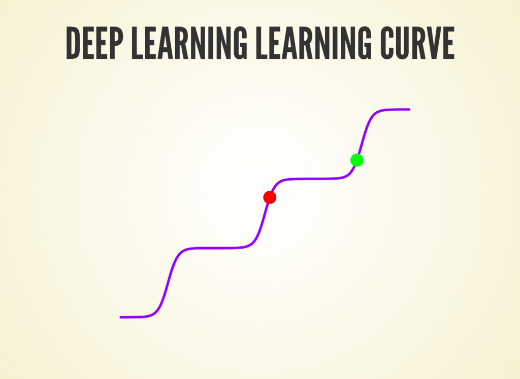
Deep learning's explosion of spectacular results over the past few years may make it appear esoteric and daunting, but in reality, if you are familiar with traditional machine learning, you're more than ready to start exploring deep learning. This talk aims to gently bridge the divide by demonstrating how deep learning operates on core machine learning concepts and getting attendees started coding deep neural networks using Google's TensorFlow library.

https://us.pycon.org/2017/schedule/presentation/2/
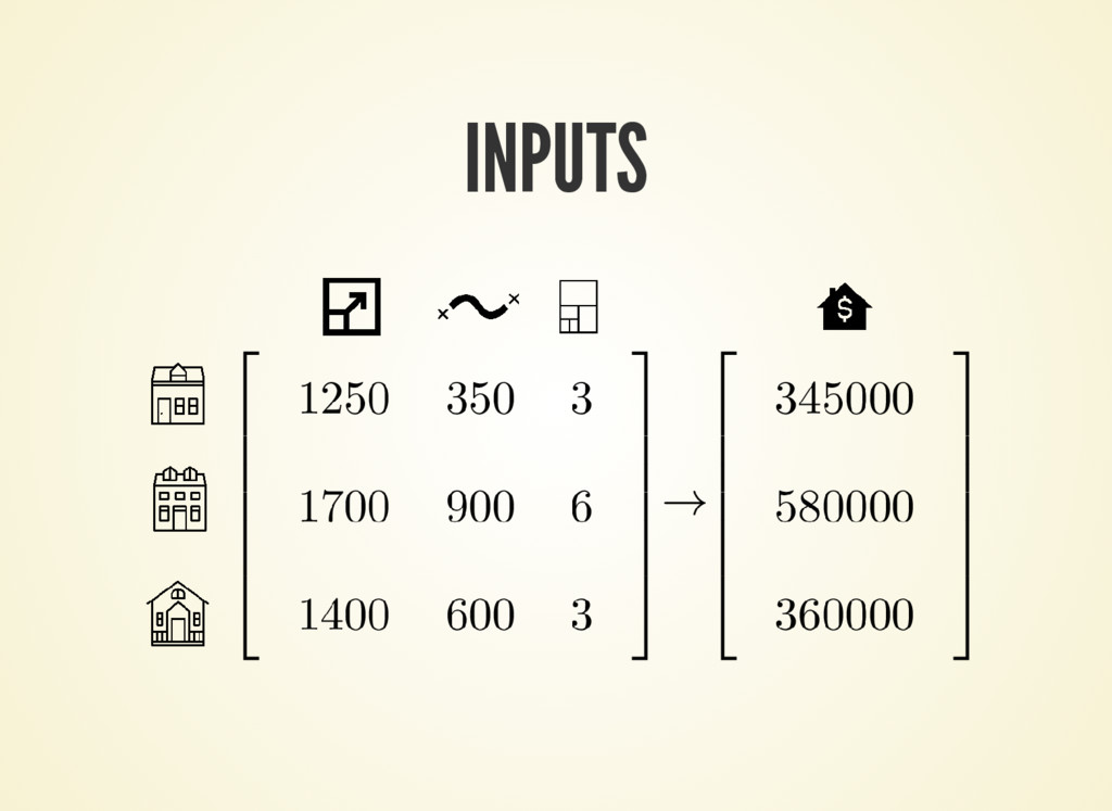
PyCon 2017

May 21, 2017
Tweet

More Decks by PyCon 2017

Other Decks in Programming

Transcript

  1. A GENTLE INTRODUCTION TO DEEP LEARNING WITH TENSORFLOW Michelle Fullwood

    @michelleful Slides: michelleful.github.io/PyCon2017
  2. TARGET (Deep) Feed-forward neural networks How they're constructed Why they

    work How to train and optimize them Image source: Fjodor van Veen (2016) Neural Network Zoo
  3. TENSORFLOW Popular deep learning toolkit From Google Brain, Apache-licensed Python

    API, makes calls to C++ back- end Works on CPUs and GPUs
  4. INPUTS X_train = np.array([ [1250, 350, 3], [1700, 900, 6],

    [1400, 600, 3] ]) Y_train = np.array([345000, 580000, 360000])
  5. MODEL Multiply each feature by a weight and add them

    up. Add an intercept to get our nal estimate.
  6. MODEL - OPERATIONS def model(X, weights, intercept): return X.dot(weights) +

    intercept Y_hat = model(X_train, weights, intercept)
  7. OPTIMIZATION - GRADIENT CALCULATION Goal: = + + + b

    y ^ w 0 x 0 w 1 x 1 w 2 x 2 ϵ = (y − y ^) 2 , ∂ϵ ∂w i ∂ϵ ∂b
  8. OPTIMIZATION - GRADIENT CALCULATION = + + + b y

    ^ w 0 x 0 w 1 x 1 w 2 x 2 = ∂y ^ ∂w 0 x 0
  9. OPTIMIZATION - GRADIENT CALCULATION = ∂y ^ ∂w 0 x

    0 = −2(y − ) dϵ dy ^ y ^ = −2(y − ) ∂ϵ ∂w 0 y ^ x 0
  10. OPTIMIZATION - GRADIENT CALCULATION = + + + b ⋅

    1 y ^ w 0 x 0 w 1 x 1 w 2 x 2 = −2(y − ) ⋅ 1 ∂ϵ ∂b y ^
  11. OPTIMIZATION - GRADIENT CALCULATION delta_y = y - y_hat gradient_weights

    = -2 * delta_y * weights gradient_intercept = -2 * delta_y * 1
  12. OPTIMIZATION - PARAMETER UPDATE learning_rate = 0.05 weights = weights

    - \ learning_rate * gradient_weights intercept = intercept - \ learning_rate * gradient_intercept
  13. TRAINING def training_round(x, y, weights, intercept, alpha=learning_rate): # calculate our

    estimate y_hat = model(x, weights, intercept) # calculate error delta_y = y - y_hat # calculate gradients gradient_weights = -2 * delta_y * weights gradient_intercept = -2 * delta_y # update parameters weights = weights - alpha * gradient_weights intercept = intercept - alpha * gradient_intercept return weights, intercept
  14. TRAINING NUM_EPOCHS = 100 def train(X, Y): # initialize parameters

    weights = np.random.randn(3) intercept = 0 # training rounds for i in range(NUM_EPOCHS): for (x, y) in zip(X, Y): weights, intercept = training_round(x, y, weights, intercept)
  15. TESTING def test(X_test, Y_test, weights, intercept): Y_predicted = model(X_test, weights,

    intercept) error = cost(Y_predicted, Y_test) return np.sqrt(np.mean(error)) >>> test(X_test, Y_test, final_weights, final_intercept) 6052.79
  16. Uh, wasn't this supposed to be a talk about neural

    networks? Why are we talking about linear regression?
  17. INPUTS → PLACEHOLDERS import tensorflow as tf X = tf.placeholder(tf.float32,

    [None, 3]) Y = tf.placeholder(tf.float32, [None, 1])
  18. PARAMETERS → VARIABLES # create tf.Variable(s) W = tf.get_variable("weights", [3,

    1], initializer=tf.random_normal_initializer()) b = tf.get_variable("intercept", [1], initializer=tf.constant_initializer(0))
  19. TRAINING with tf.Session() as sess: # initialize variables sess.run(tf.global_variables_initializer()) #

    train for _ in range(NUM_EPOCHS): for (X_batch, Y_batch) in get_minibatches( X_train, Y_train, BATCH_SIZE): sess.run(optimizer, feed_dict={ X: X_batch, Y: Y_batch })
  20. TRAINING with tf.Session() as sess: # initialize variables sess.run(tf.global_variables_initializer()) #

    train for _ in range(NUM_EPOCHS): for (X_batch, Y_batch) in get_minibatches( X_train, Y_train, BATCH_SIZE): sess.run(optimizer, feed_dict={ X: X_batch, Y: Y_batch })
  21. TRAINING with tf.Session() as sess: # initialize variables sess.run(tf.global_variables_initializer()) #

    train for _ in range(NUM_EPOCHS): for (X_batch, Y_batch) in get_minibatches( X_train, Y_train, BATCH_SIZE): sess.run(optimizer, feed_dict={ X: X_batch, Y: Y_batch })
  22. TRAINING with tf.Session() as sess: # initialize variables sess.run(tf.global_variables_initializer()) #

    train for _ in range(NUM_EPOCHS): for (X_batch, Y_batch) in get_minibatches( X_train, Y_train, BATCH_SIZE): sess.run(optimizer, feed_dict={ X: X_batch, Y: Y_batch })
  23. # Placeholders X = tf.placeholder(tf.float32, [None, 3]) Y = tf.placeholder(tf.float32,

    [None, 1]) # Parameters/Variables W = tf.get_variable("weights", [3, 1], initializer=tf.random_normal_initializer()) b = tf.get_variable("intercept", [1], initializer=tf.constant_initializer(0)) # Operations Y_hat = tf.matmul(X, W) + b # Cost function cost = tf.reduce_mean(tf.square(Y_hat - Y)) # Optimization optimizer = tf.train.GradientDescentOptimizer (learning_rate).minimize(cost) # ------------------------------------------------ # Train with tf.Session() as sess: # initialize variables sess.run(tf.global_variables_initializer()) # run training rounds for _ in range(NUM_EPOCHS): for X_batch, Y_batch in get_minibatches( X_train, Y_train, BATCH_SIZE): sess.run(optimizer, feed_dict={X: X_batch, Y: Y_batch})
  24. FORWARD PROPAGATION def training_round(x, y, weights, intercept, alpha=learning_rate): # calculate

    our estimate y_hat = model(x, weights, intercept) # calculate error delta_y = y - y_hat # calculate gradients gradient_weights = -2 * delta_y * weights gradient_intercept = -2 * delta_y # update parameters weights = weights - alpha * gradient_weights intercept = intercept - alpha * gradient_intercept return weights, intercept
  25. BACKPROPAGATION def training_round(x, y, weights, intercept, alpha=learning_rate): # calculate our

    estimate y_hat = model(x, weights, intercept) # calculate error delta_y = y - y_hat # calculate gradients gradient_weights = -2 * delta_y * weights gradient_intercept = -2 * delta_y # update parameters weights = weights - alpha * gradient_weights intercept = intercept - alpha * gradient_intercept return weights, intercept
  26. VARIABLE UPDATE def training_round(x, y, weights, intercept, alpha=learning_rate): # calculate

    our estimate y_hat = model(x, weights, intercept) # calculate error delta_y = y - y_hat # calculate gradients gradient_weights = -2 * delta_y * weights gradient_intercept = -2 * delta_y # update parameters weights = weights - alpha * gradient_weights intercept = intercept - alpha * gradient_intercept return weights, intercept
  27. TESTING with tf.Session() as sess: # train # ... (code

    from above) # test Y_predicted = sess.run(model, feed_dict = {X: X_test}) squared_error = tf.reduce_mean( tf.square(Y_test, Y_predicted)) >>> np.sqrt(squared_error) 5967.39
  28. BINARY LOGISTIC REGRESSION - MODEL Take a weighted sum of

    the features and add a bias term to get the logit. Convert the logit to a probability via the logistic-sigmoid function.
  29. PLACEHOLDERS # X = vector length 784 (= 28 x

    28 pixels) # Y = one-hot vectors # digit 0 = [1, 0, 0, 0, 0, 0, 0, 0, 0, 0] X = tf.placeholder(tf.float32, [None, 28*28]) Y = tf.placeholder(tf.float32, [None, 10])
  30. TRAINING with tf.Session() as sess: sess.run(tf.global_variables_initializer()) for i in range(NUM_EPOCHS):

    for (X_batch, Y_batch) in get_minibatches( X_train, Y_train, BATCH_SIZE): sess.run(optimizer, feed_dict={X: X_batch, Y: Y_batch})
  31. TESTING predict = tf.argmax(Y_logits, 1) with tf.Session() as sess: #

    training code from above predictions = sess.run(predict, feed_dict={X: X_test}) accuracy = tf.reduce_mean(np.mean( np.argmax(Y_test, axis=1) == predictions) >>> accuracy 0.925
  32. ADDING ANOTHER LAYER - VARIABLES HIDDEN_NODES = 128 W1 =

    tf.get_variable("weights1", [784, HIDDEN_NODES], initializer=tf.random_normal_initializer()) b1 = tf.get_variable("bias1", [HIDDEN_NODES], initializer=tf.constant_initializer(0)) W2 = tf.get_variable("weights2", [HIDDEN_NODES, 10], initializer=tf.random_normal_initializer()) b2 = tf.get_variable("bias2", [10], initializer=tf.constant_initializer(0))
  33. ADDING ANOTHER LAYER - OPERATIONS hidden = tf.matmul(X, W1) +

    b1 y_logits = tf.matmul(hidden, W2) + b2
  34. PROBLEM A linear transformation of a linear transformation is still

    a linear transformation! We need to add non-linearity to the system.
  35. UNIVERSAL APPROXIMATION THEOREM A feedforward network with a single hidden

    layer containing a nite number of neurons can approximate (basically) any interesting function
  36. WHY GO DEEP? 3 reasons: Deeper networks are more powerful

    Narrower networks are less prone to over tting