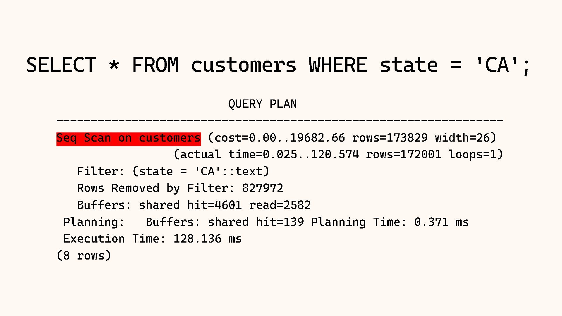
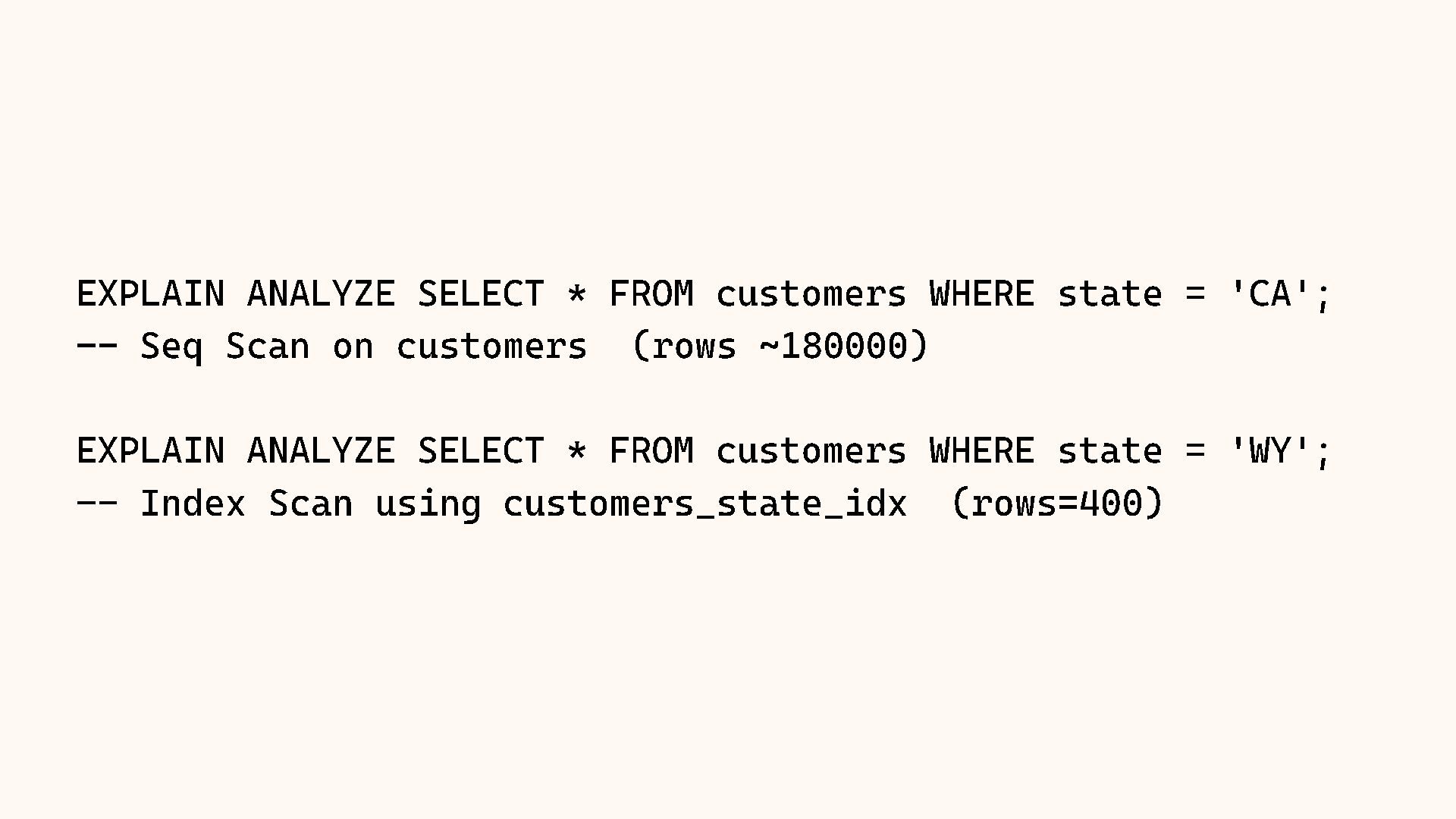
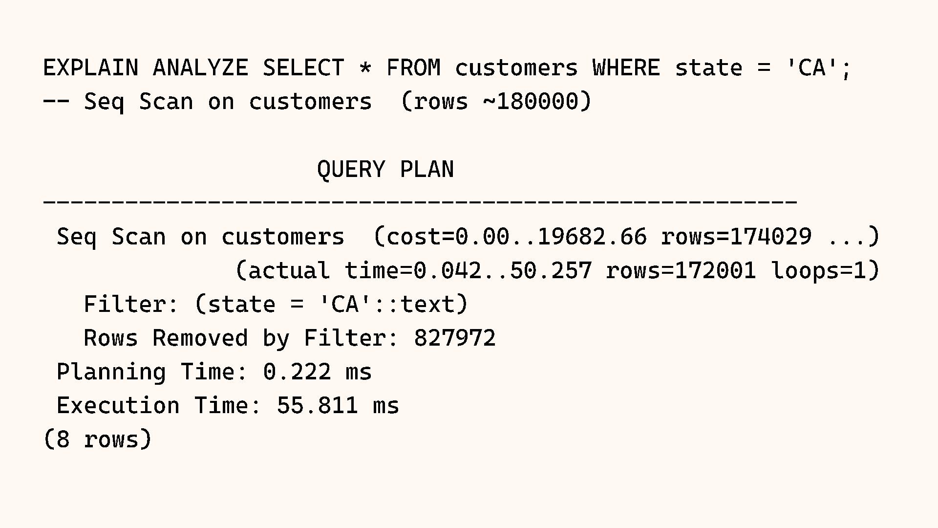
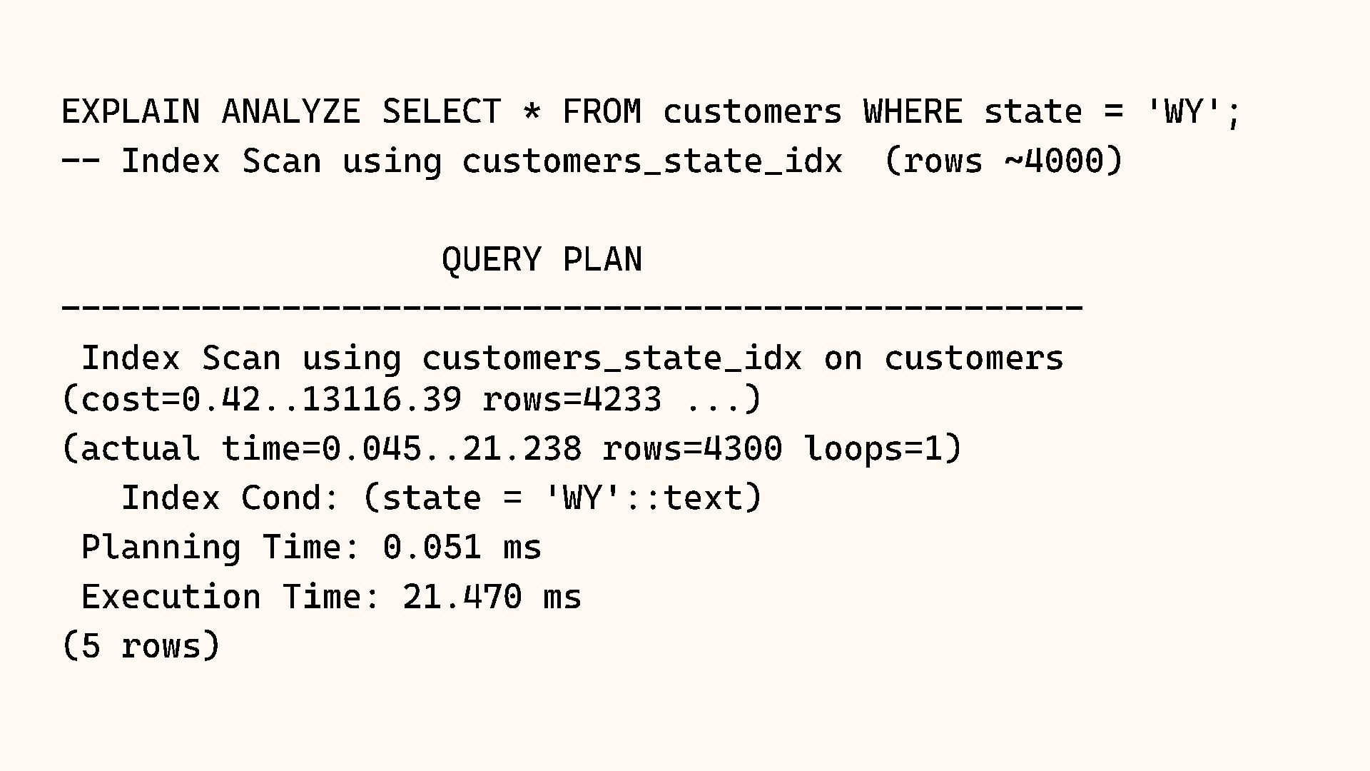
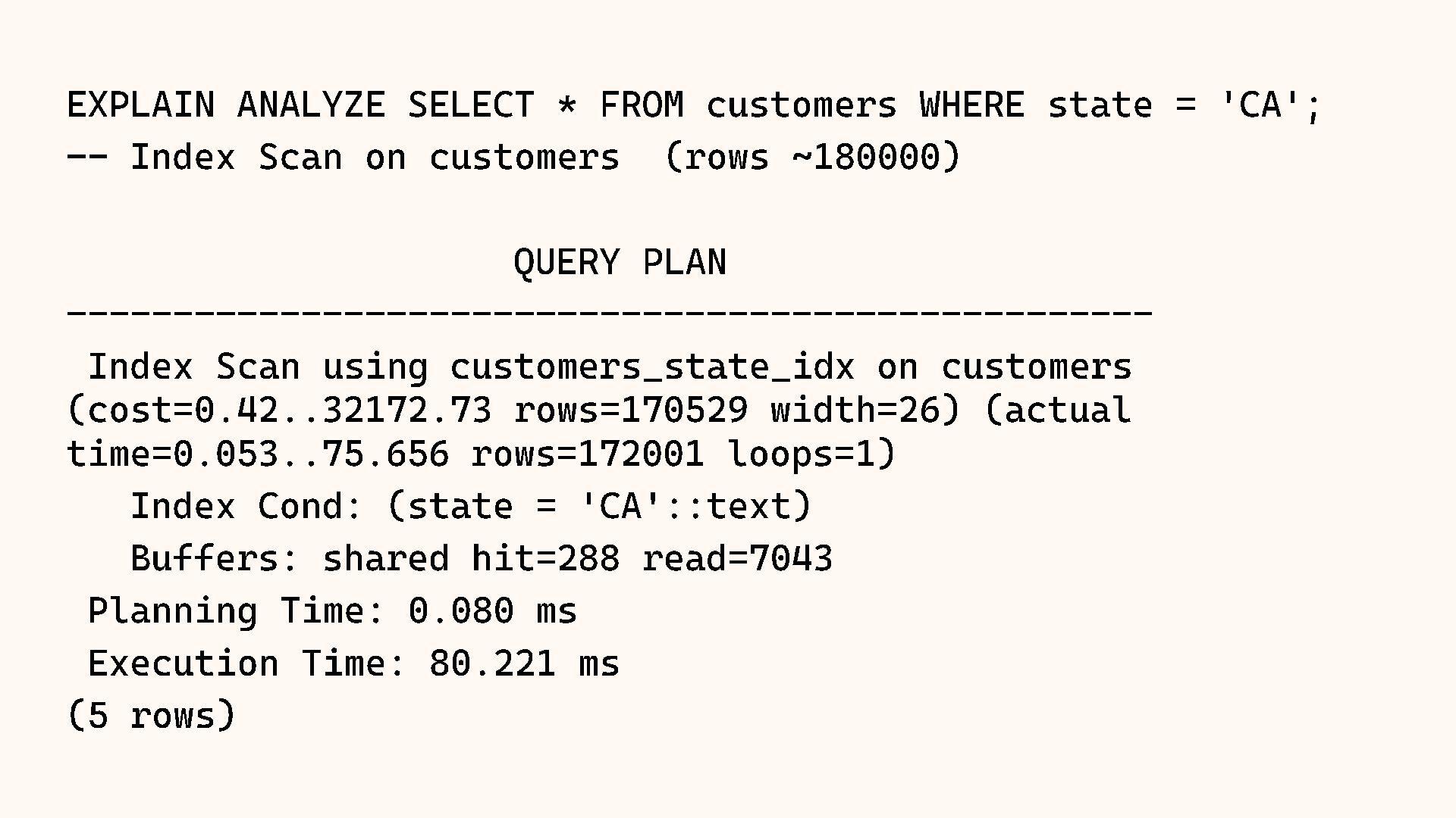
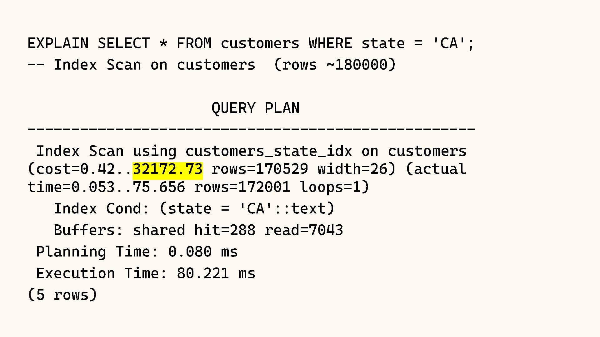
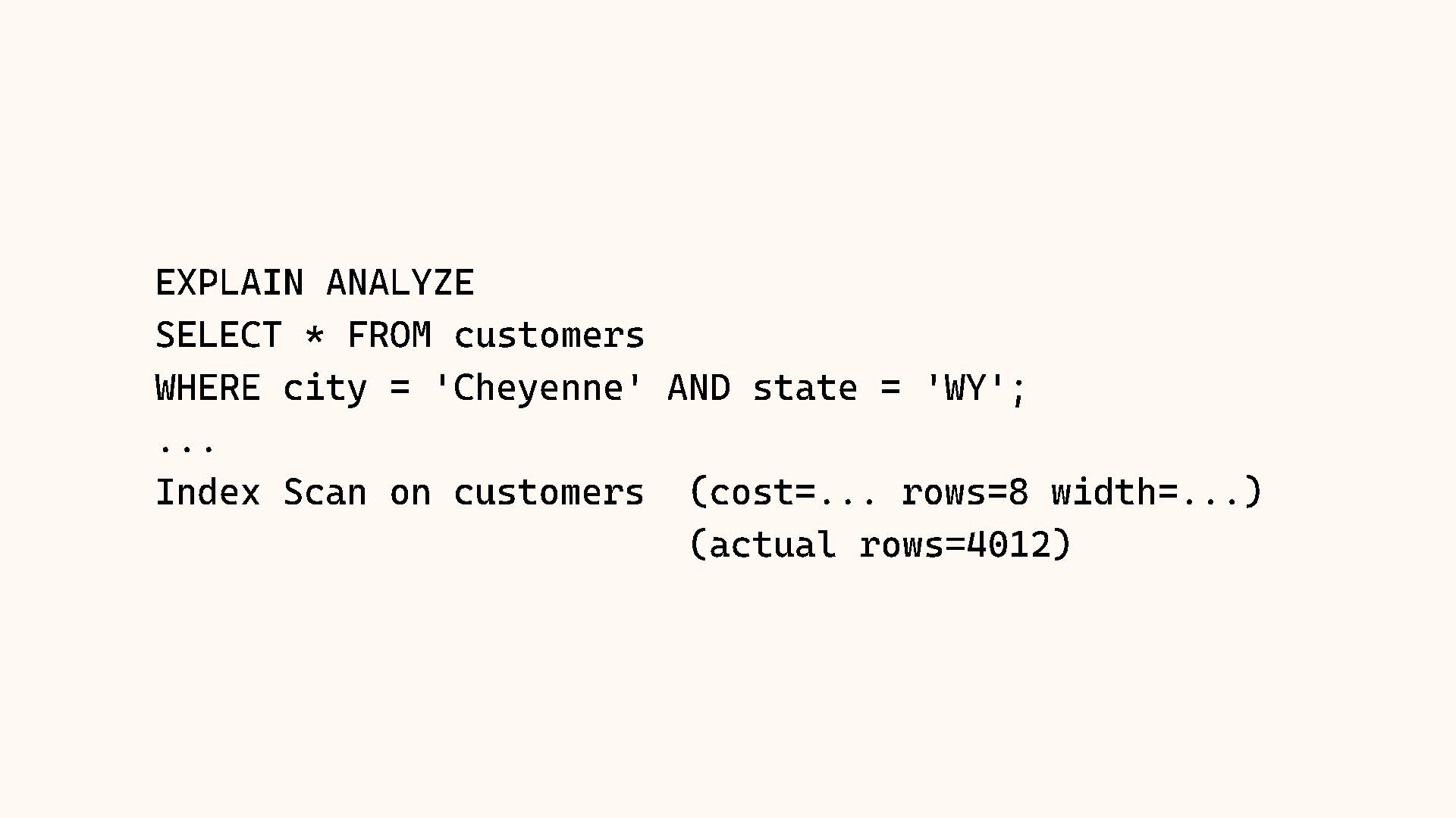
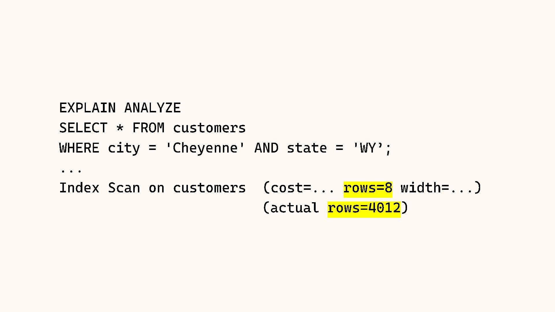
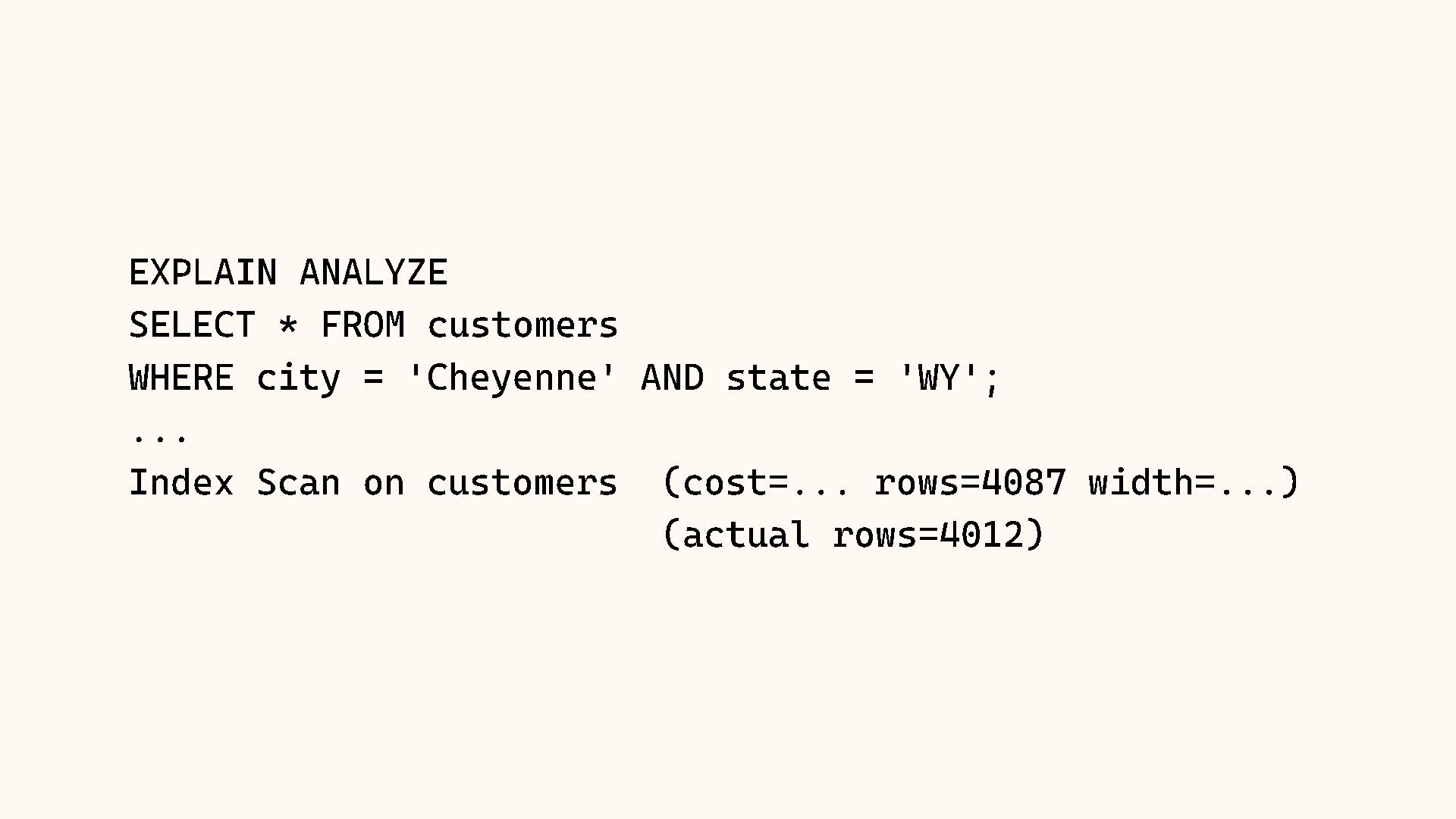
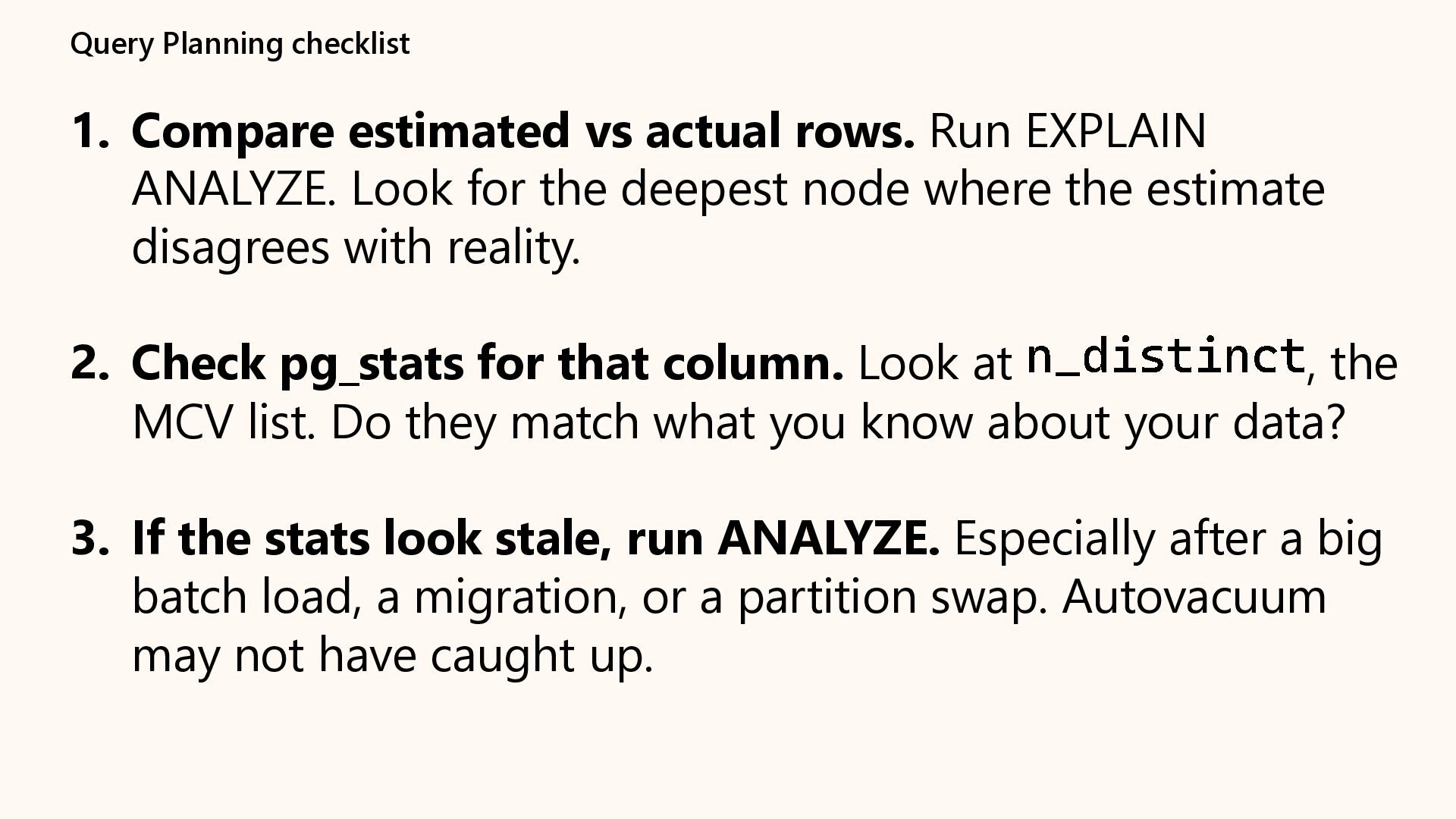
Why does Postgres sometimes choose a Sequential Scan over an Index Scan, even when it seems slower? The answer almost always lies in the statistics. The query planner relies on a mathematical model of your data distribution to make decisions, and when that model is wrong, performance suffers.
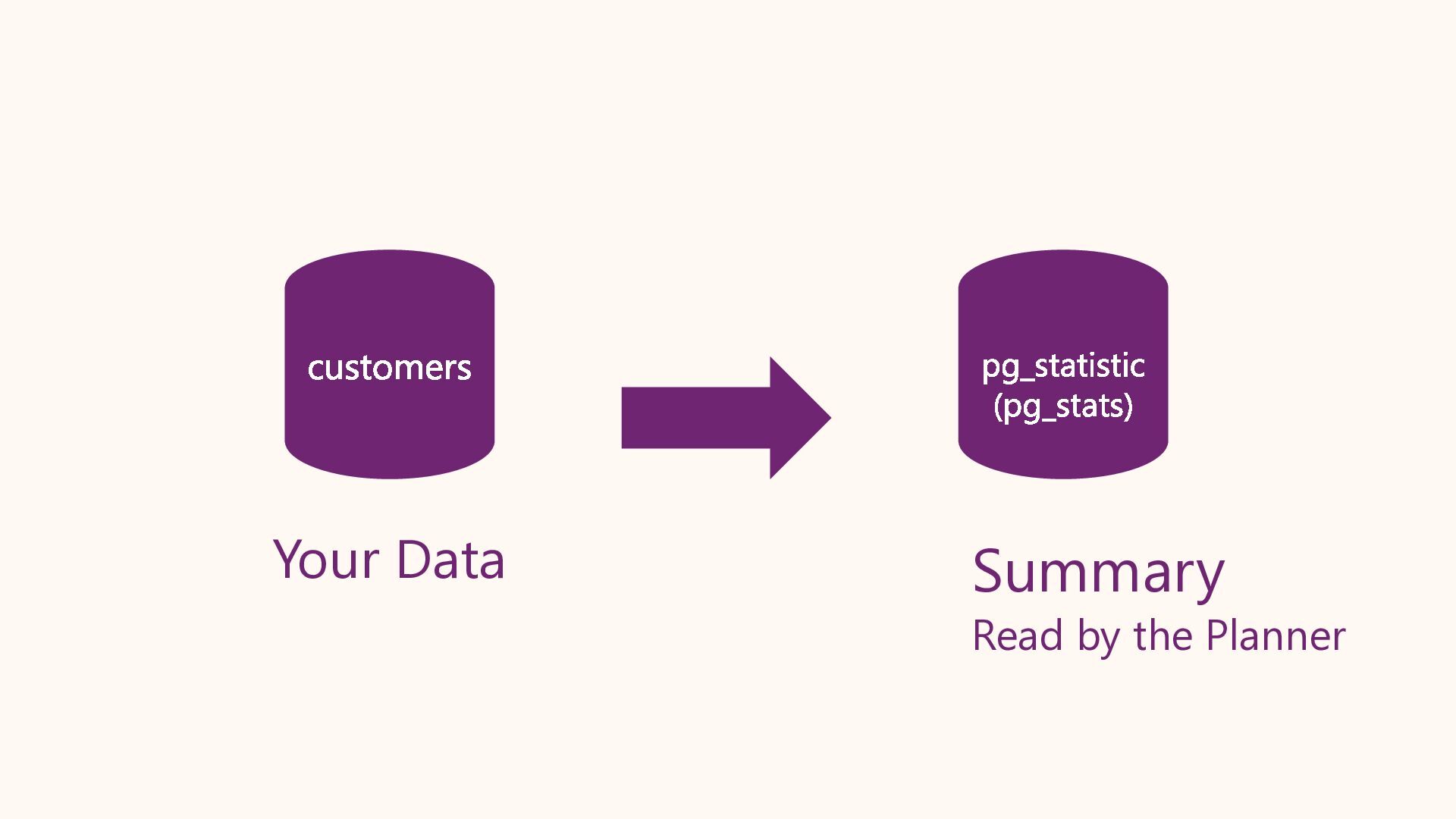
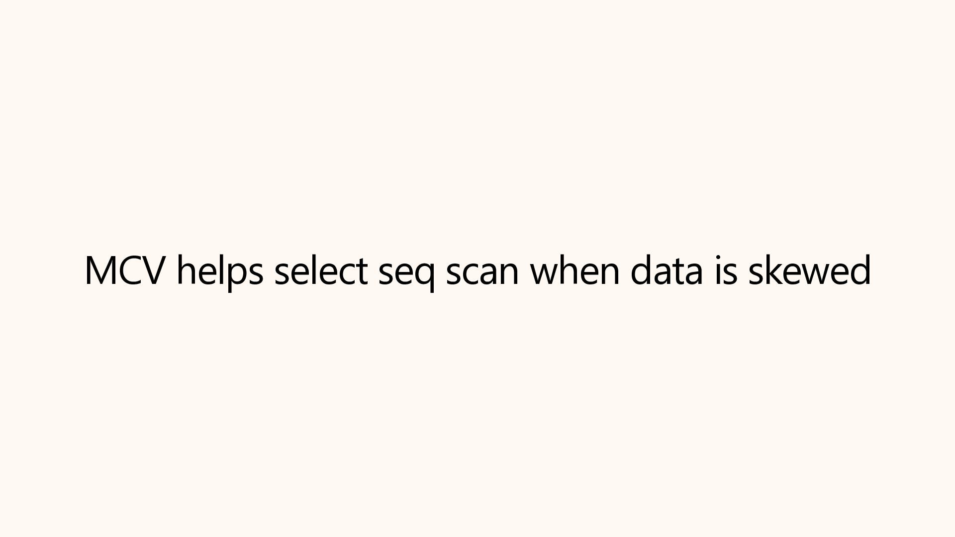
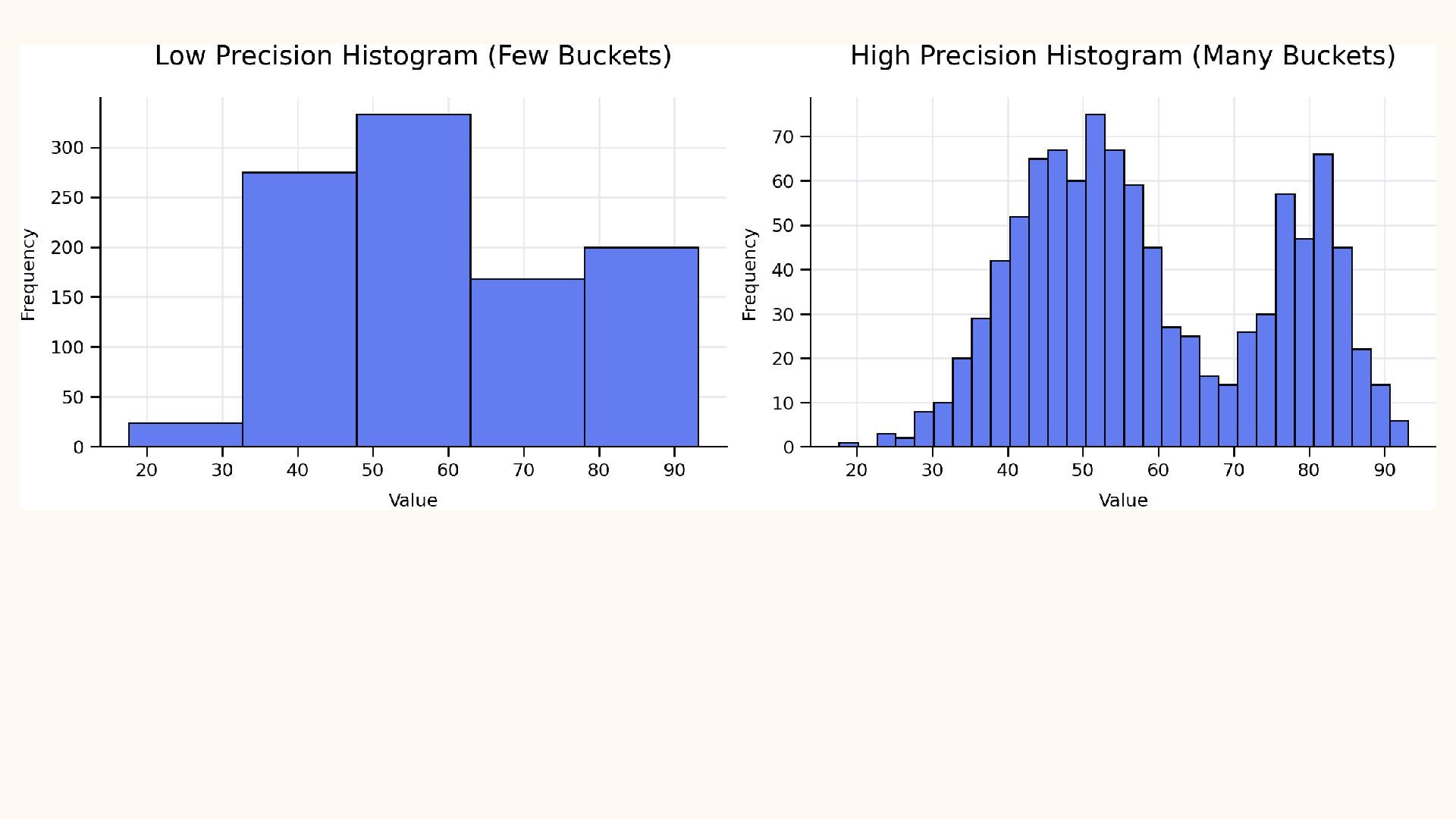
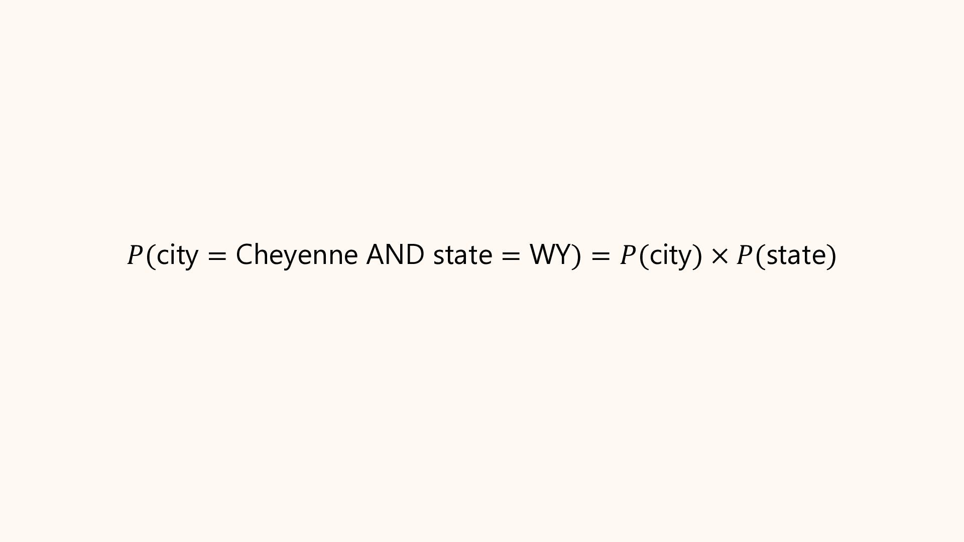
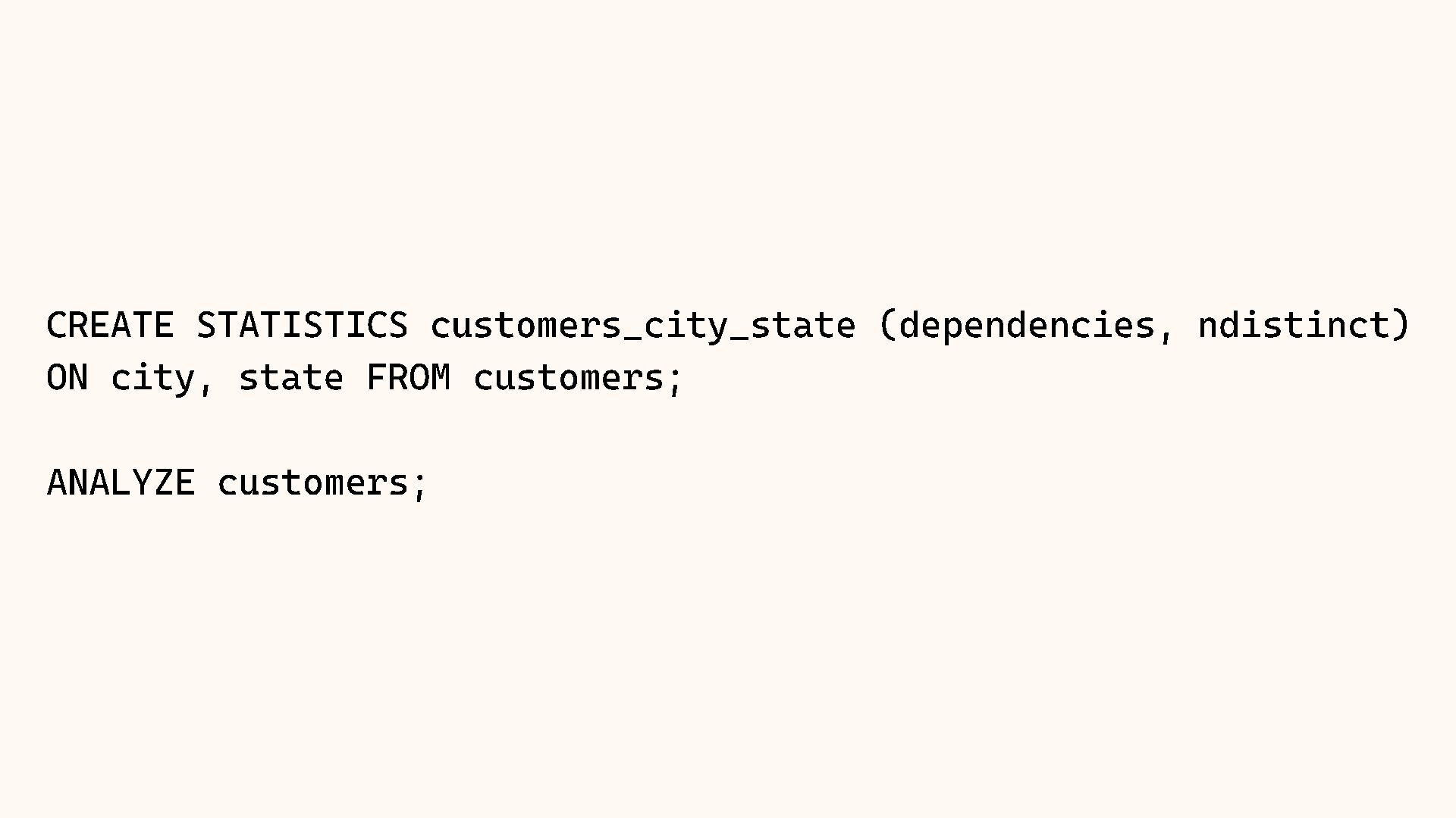
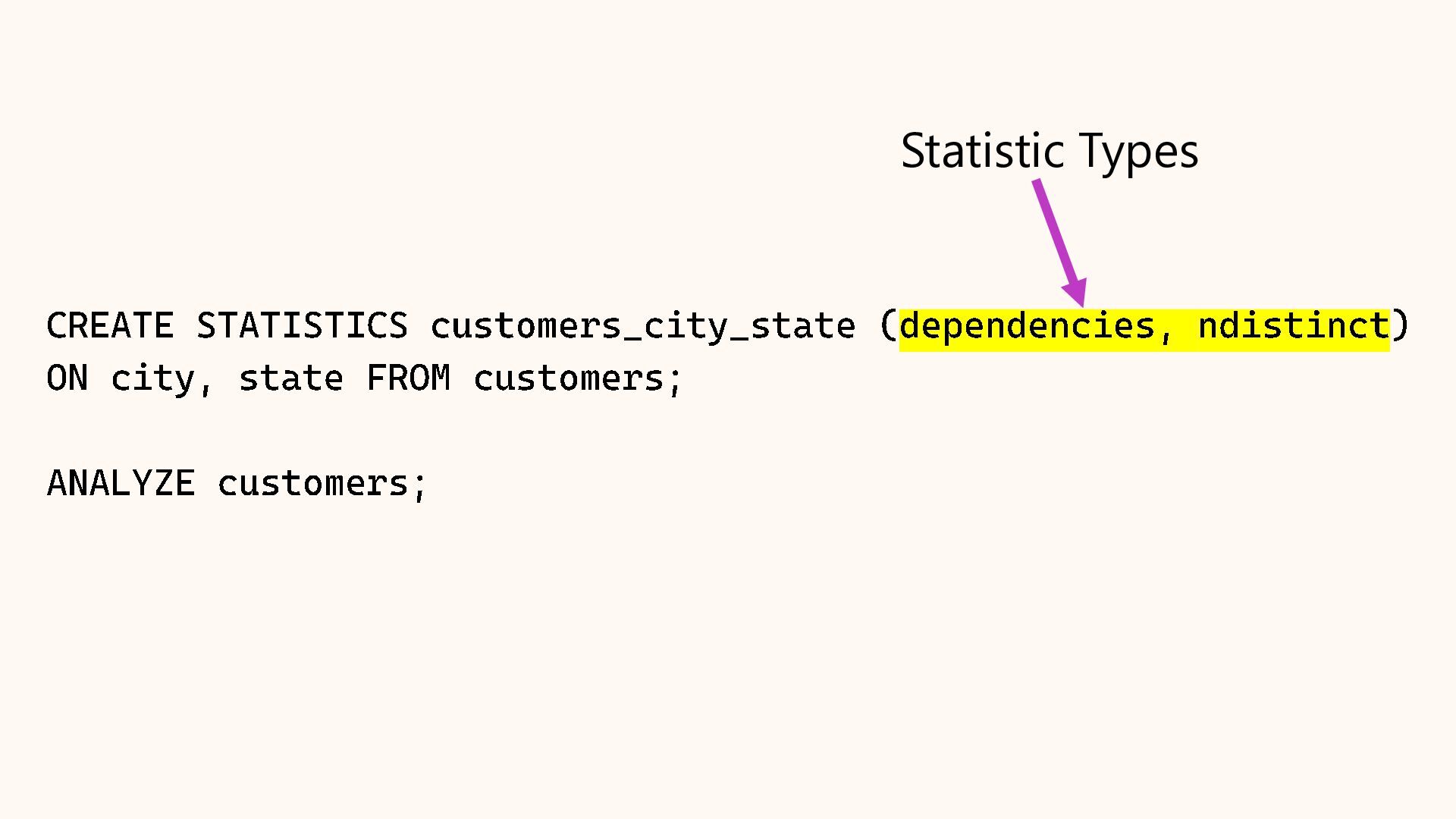
In this session, we will crack open the pg_stats view to understand exactly how Postgres "sees" your data. We will cover histograms, most common values (MCV), and correlation. We will also explore Extended Statistics, a powerful feature for fixing bad query plans on correlated columns (like City and State), ensuring your planner stops guessing and starts knowing.
As presented at POSETTE 2026 Livestream #2
June 16, 2026
![SELECT unnest( most_common_vals ::text::text[]) AS state, unnest( most_common_freqs ) AS](https://files.speakerdeck.com/presentations/dbf844350eb84e52af62404524ef13bd/slide_16.jpg)
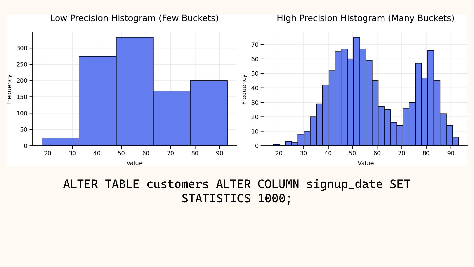
![SELECT (unnest( histogram_bounds ::text::date[]))::date AS bucket_bound FROM pg_stats WHERE tablename](https://files.speakerdeck.com/presentations/dbf844350eb84e52af62404524ef13bd/slide_27.jpg)
![SELECT (unnest( histogram_bounds ::text::date[]))::date AS bucket_bound FROM pg_stats WHERE tablename](https://files.speakerdeck.com/presentations/dbf844350eb84e52af62404524ef13bd/slide_30.jpg)
![SELECT (unnest( histogram_bounds ::text::date[]))::date AS bucket_bound FROM pg_stats WHERE tablename](https://files.speakerdeck.com/presentations/dbf844350eb84e52af62404524ef13bd/slide_31.jpg)