Shinsaku Sakaue (Univ. Tokyo, RIKEN AIP) Joint work with Taira Tsuchiya (Univ. Tokyo, RIKEN AIP), Han Bao (Kyoto Univ.), Taihei Oki (Hokkaido Univ.) Preprint: https://arxiv.org/abs/2501.14349
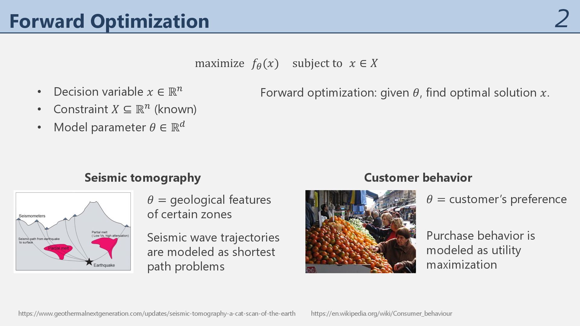
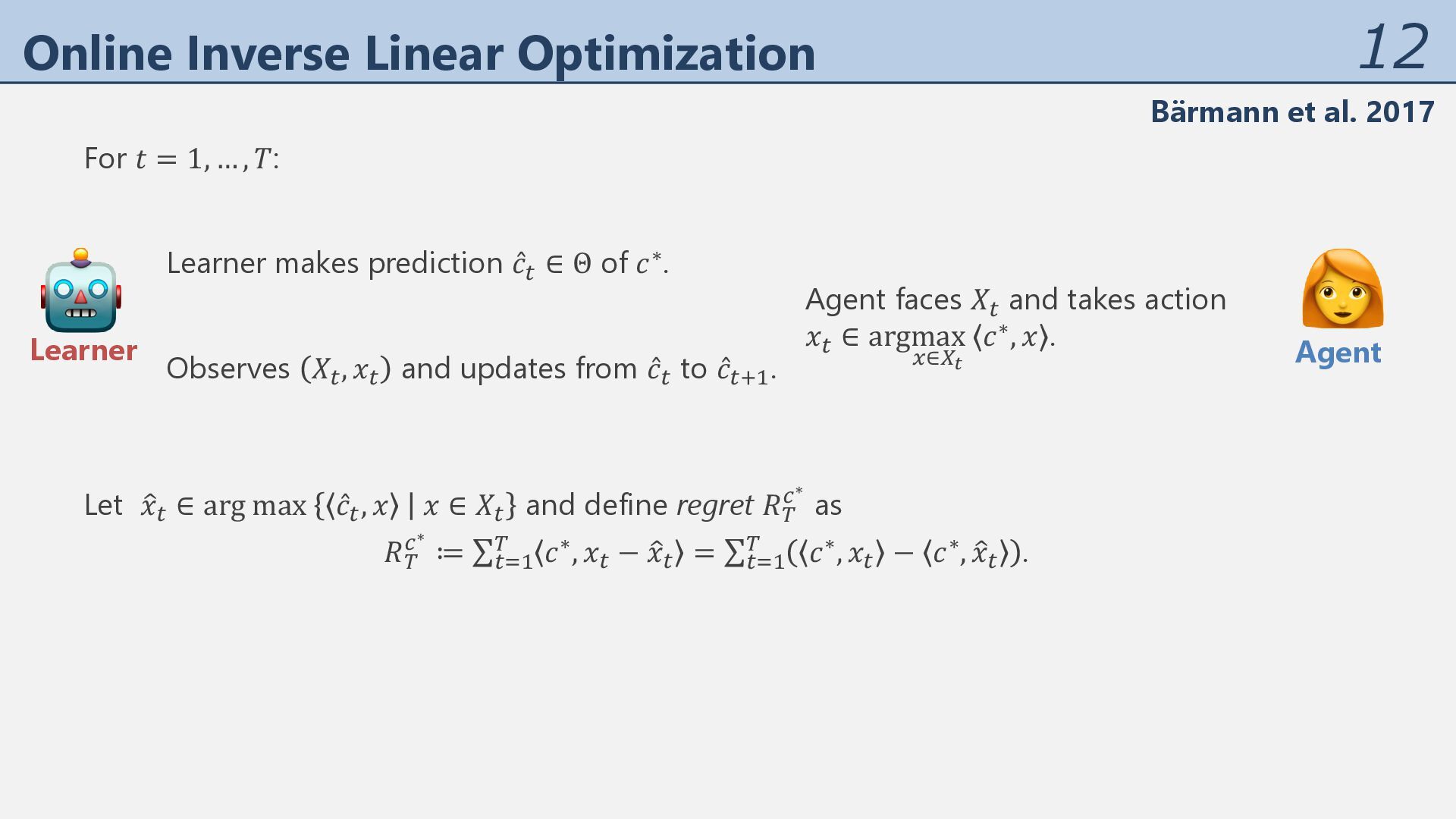
= 1, … , 𝑇, an agent solves maximize 𝑐∗, 𝑥 subject to 𝑥 ∈ 𝑋% . Budget = 2 𝑐∗ = 0.2 0.4 0.1 0.0 0.3 👩🦰 Agent • 𝑐∗ ∈ ℝ" is the agent’s internal objective vector. • 𝑐∗ lies in a convex set Θ ⊂ ℝ" with diam Θ = 1 (known to the learner). • 𝑋% ⊆ ℝ" is the agent’s 𝑡th action set with diam 𝑋% = 1. – not necessarily convex, but we assume an oracle to solve linear optimization on 𝑋! . • Let 𝑥% ∈ arg max 𝑐∗, 𝑥 𝑥 ∈ 𝑋% .
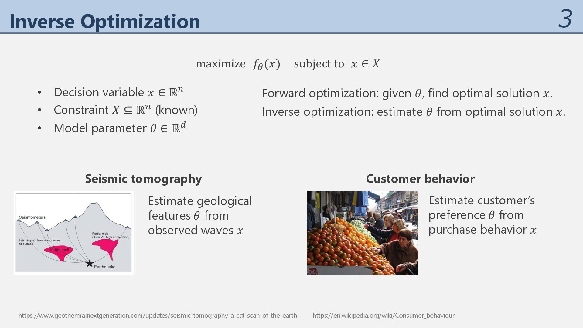
= 1, … , 𝑇, an agent solves maximize 𝑐∗, 𝑥 subject to 𝑥 ∈ 𝑋% . 𝑋% Sold out 𝑐∗ = 0.2 0.4 0.1 0.0 0.3 👩🦰 Agent Budget = 2 • 𝑐∗ ∈ ℝ" is the agent’s internal objective vector. • 𝑐∗ lies in a convex set Θ ⊂ ℝ" with diam Θ = 1 (known to the learner). • 𝑋% ⊆ ℝ" is the agent’s 𝑡th action set with diam 𝑋% = 1. – not necessarily convex, but we assume an oracle to solve linear optimization on 𝑋! . • Let 𝑥% ∈ arg max 𝑐∗, 𝑥 𝑥 ∈ 𝑋% .
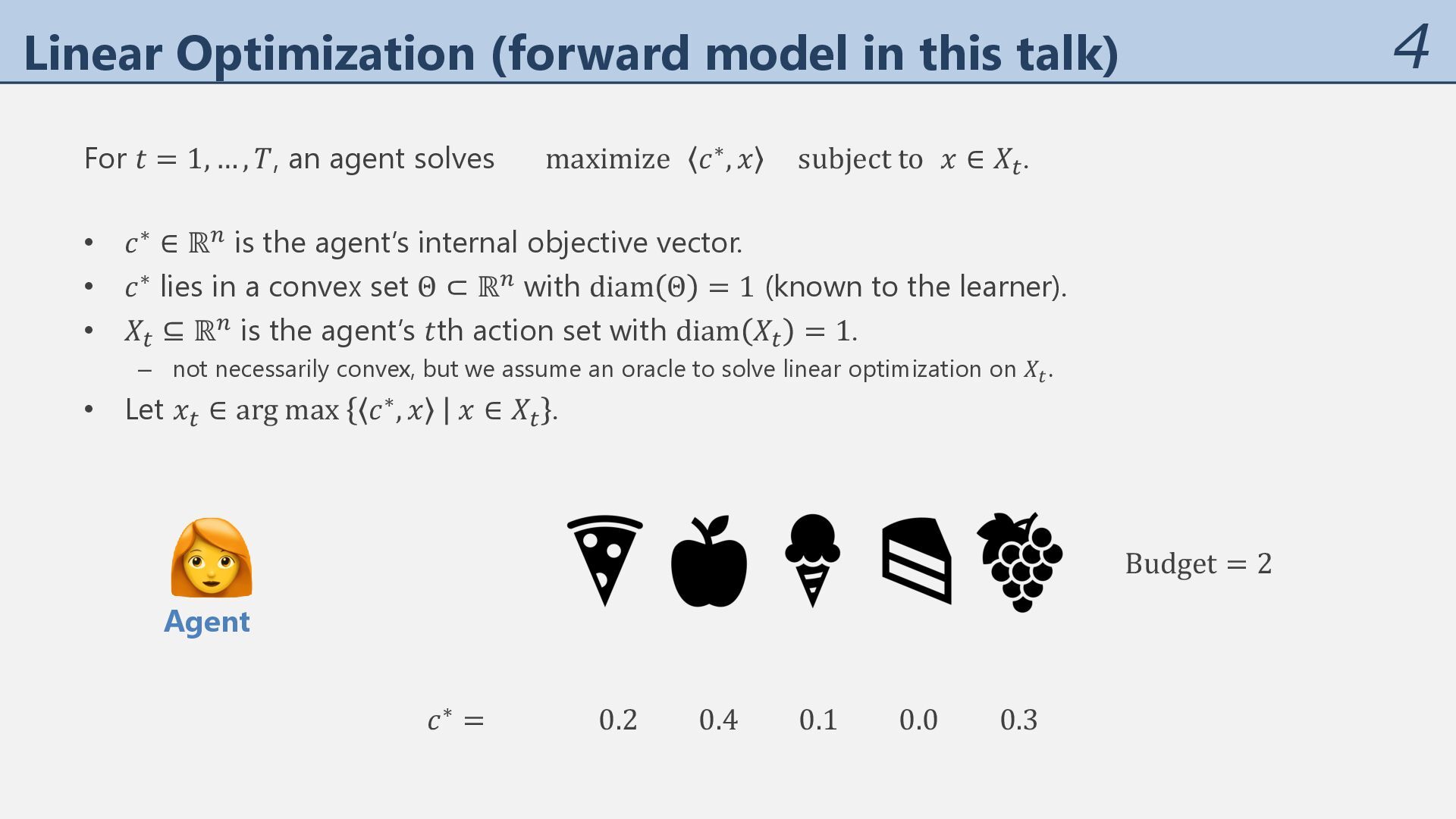
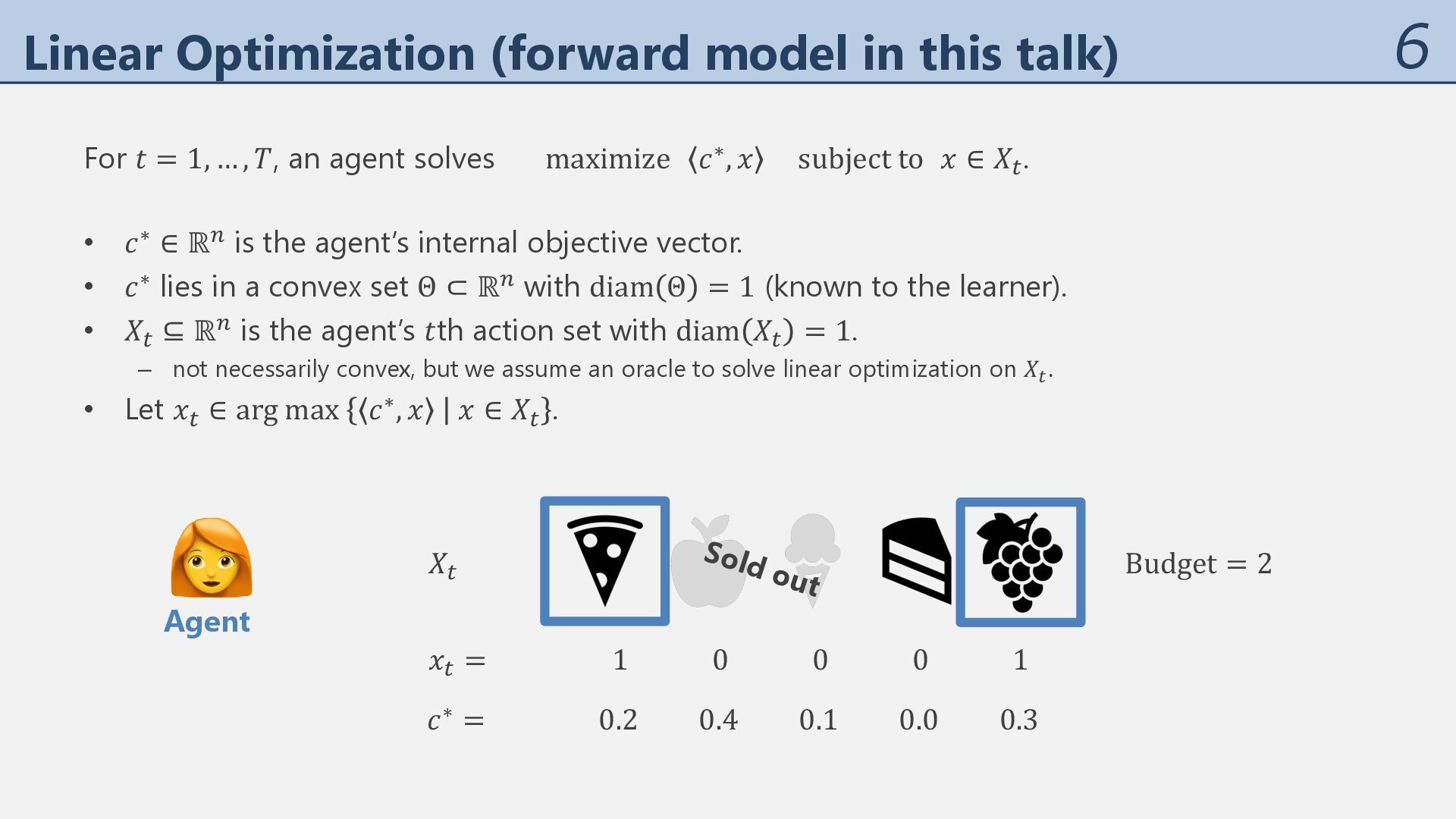
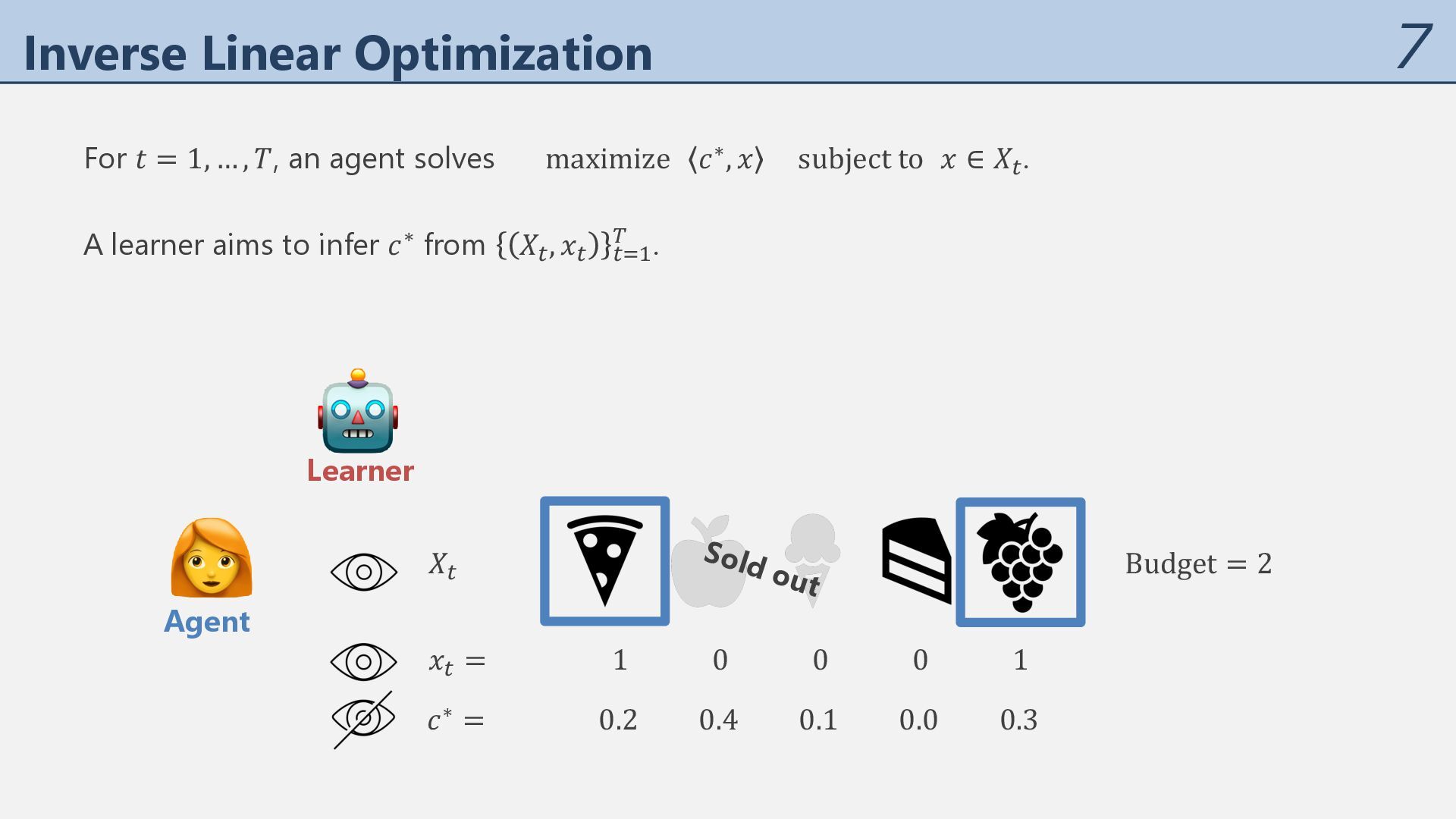
= 1, … , 𝑇, an agent solves maximize 𝑐∗, 𝑥 subject to 𝑥 ∈ 𝑋% . 𝑋% Sold out 𝑥% = 1 0 0 0 1 𝑐∗ = 0.2 0.4 0.1 0.0 0.3 👩🦰 Agent Budget = 2 • 𝑐∗ ∈ ℝ" is the agent’s internal objective vector. • 𝑐∗ lies in a convex set Θ ⊂ ℝ" with diam Θ = 1 (known to the learner). • 𝑋% ⊆ ℝ" is the agent’s 𝑡th action set with diam 𝑋% = 1. – not necessarily convex, but we assume an oracle to solve linear optimization on 𝑋! . • Let 𝑥% ∈ arg max 𝑐∗, 𝑥 𝑥 ∈ 𝑋% .
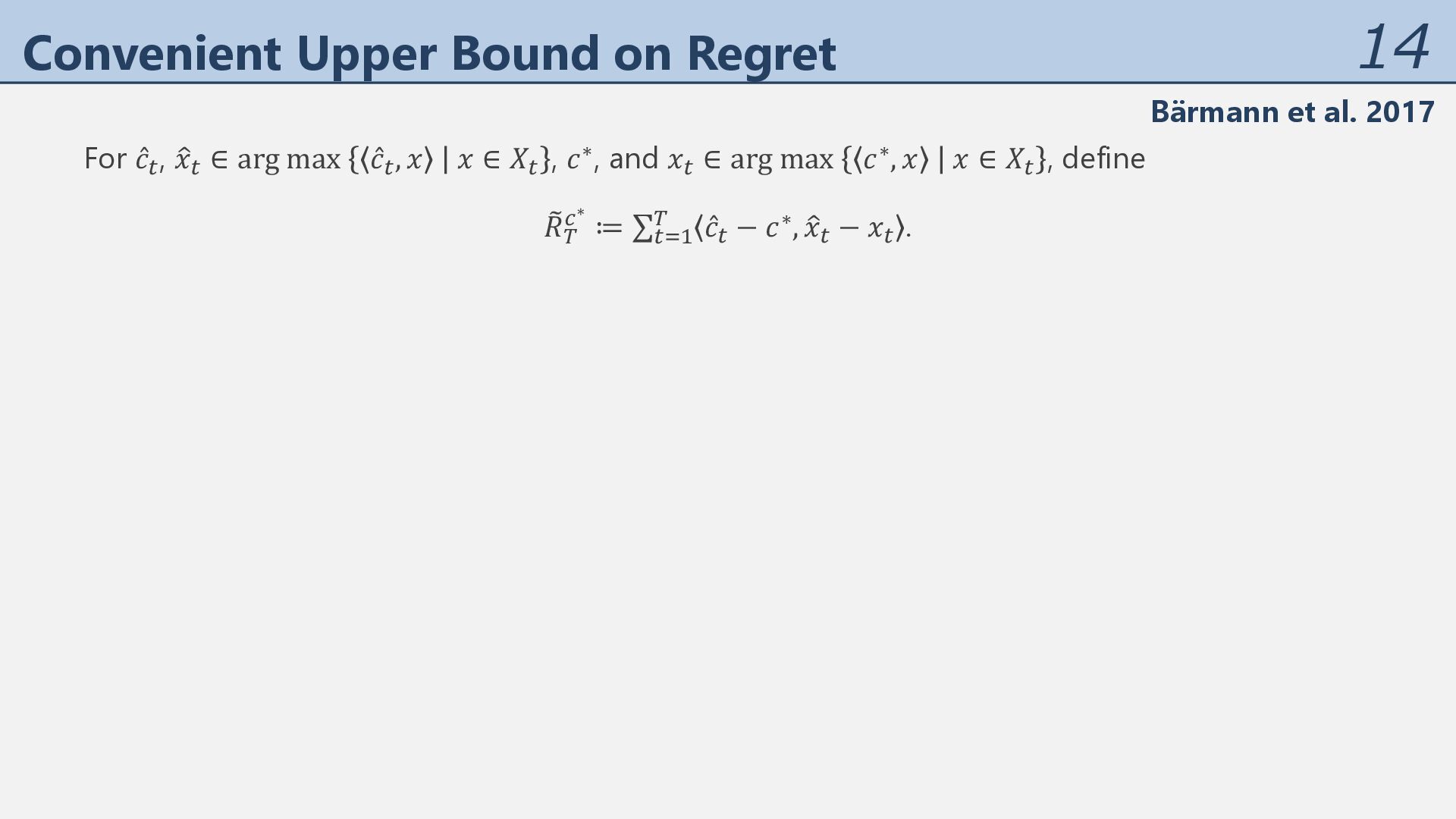
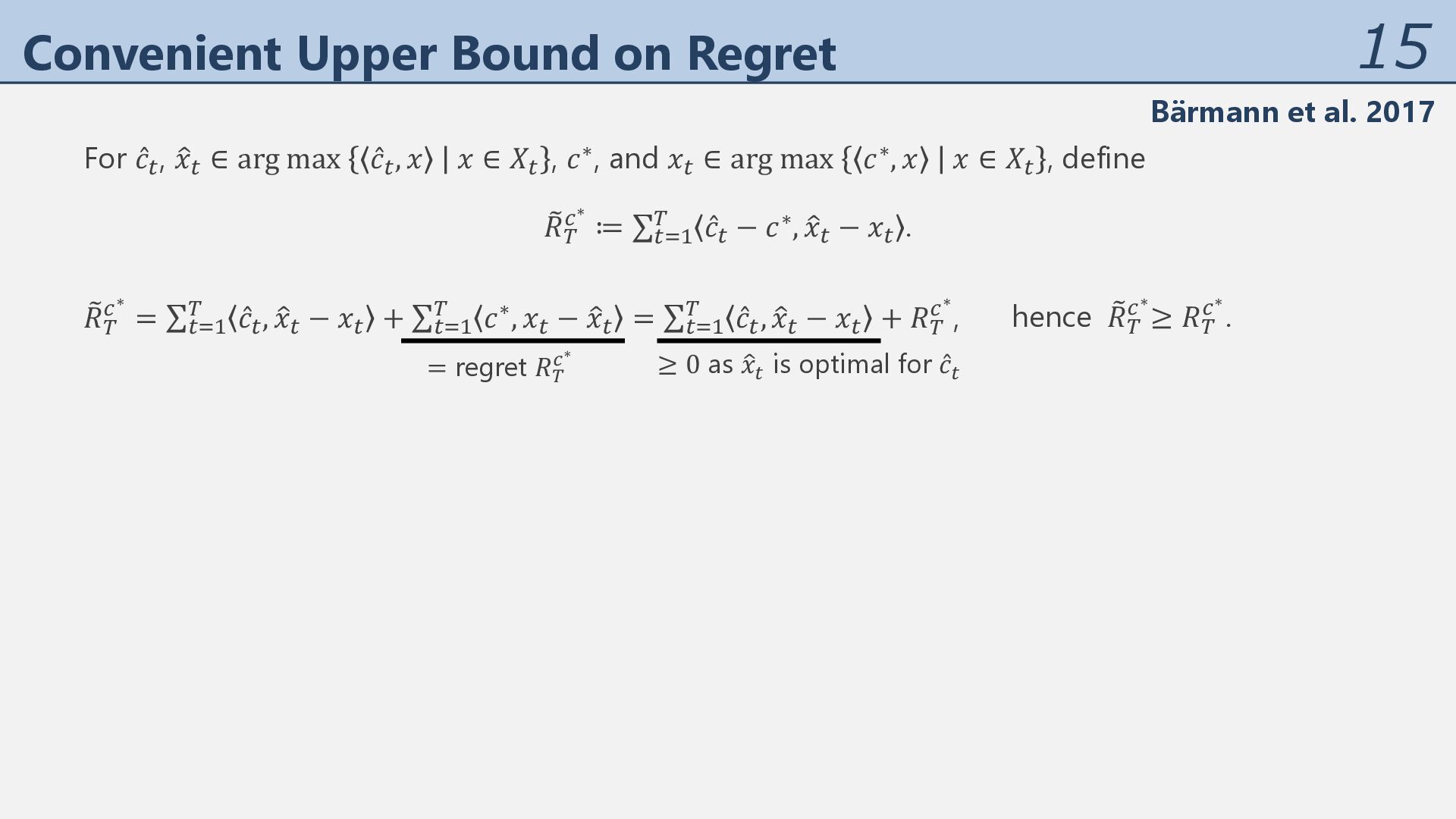
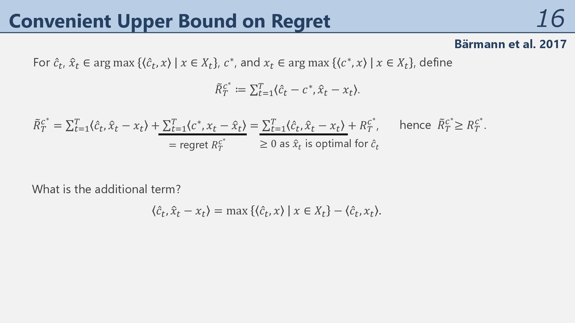
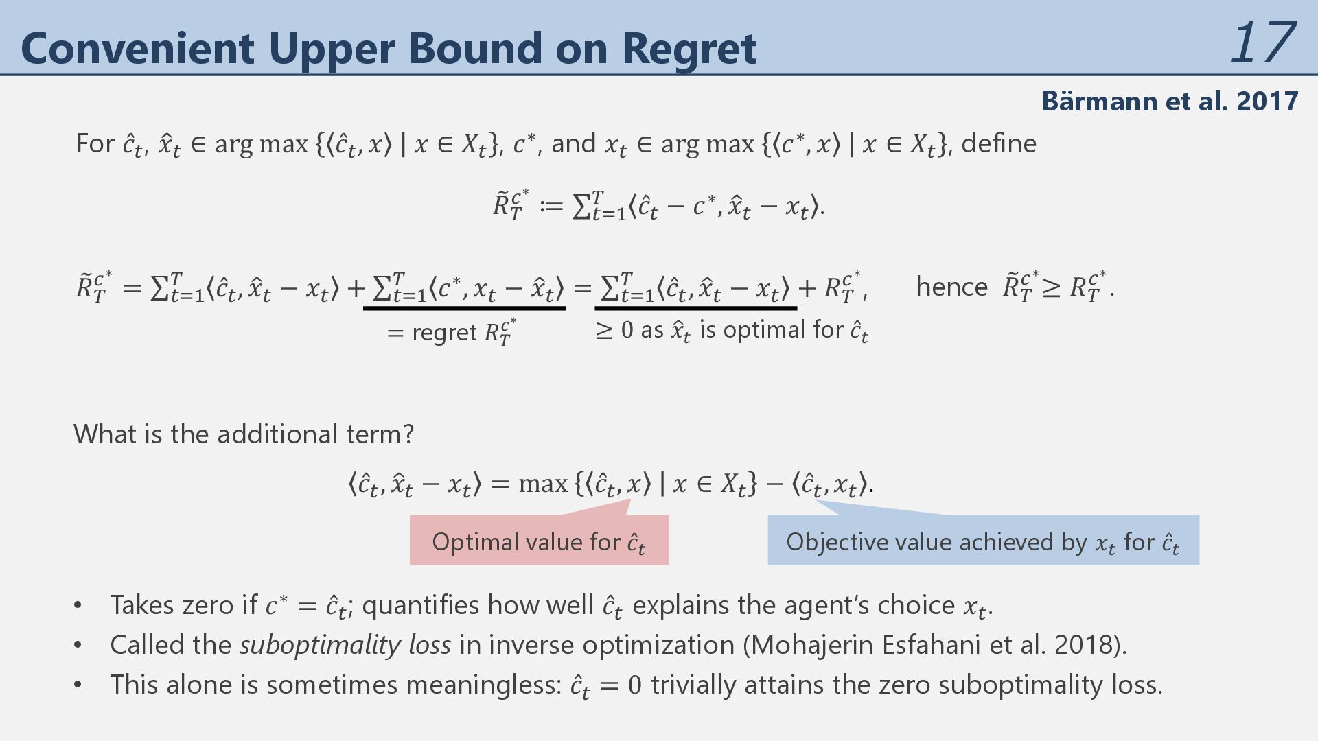
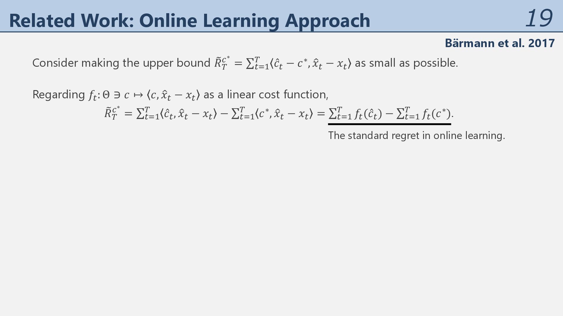
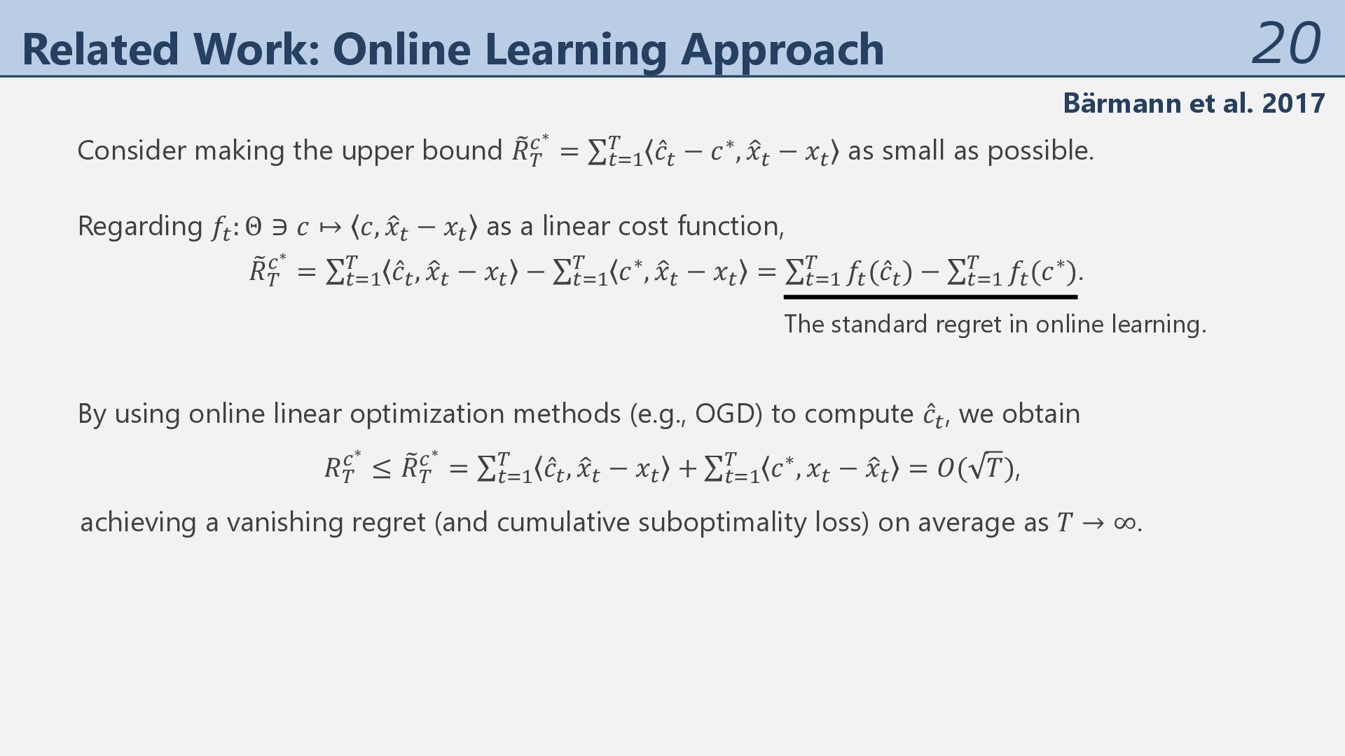
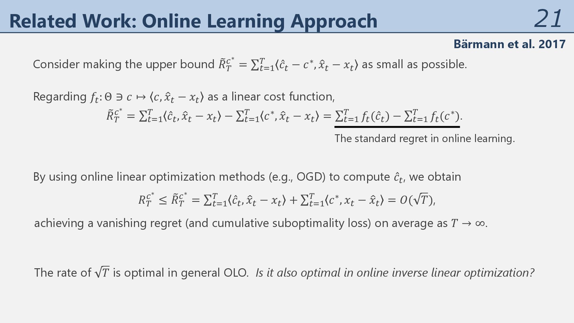
bound O 𝑅( -∗ = ∑%&' ( ̂ 𝑐% − 𝑐∗, J 𝑥% − 𝑥% as small as possible. The standard regret in online learning. By using online linear optimization methods (e.g., OGD) to compute ̂ 𝑐% , we obtain 𝑅( -∗ ≤ O 𝑅( -∗ = ∑%&' ( ̂ 𝑐%, J 𝑥% − 𝑥% + ∑%&' ( 𝑐∗, 𝑥% − J 𝑥% = 𝑂( 𝑇), achieving a vanishing regret (and cumulative suboptimality loss) on average as 𝑇 → ∞. The rate of 𝑇 is optimal in general OLO. Is it also optimal in online inverse linear optimization? Regarding 𝑓%: Θ ∋ 𝑐 ↦ 𝑐, J 𝑥% − 𝑥% as a linear cost function, O 𝑅( -∗ = ∑%&' ( ̂ 𝑐%, J 𝑥% − 𝑥% − ∑%&' ( 𝑐∗, J 𝑥% − 𝑥% = ∑%&' ( 𝑓%( ̂ 𝑐%) − ∑%&' ( 𝑓%(𝑐∗). Bärmann et al. 2017
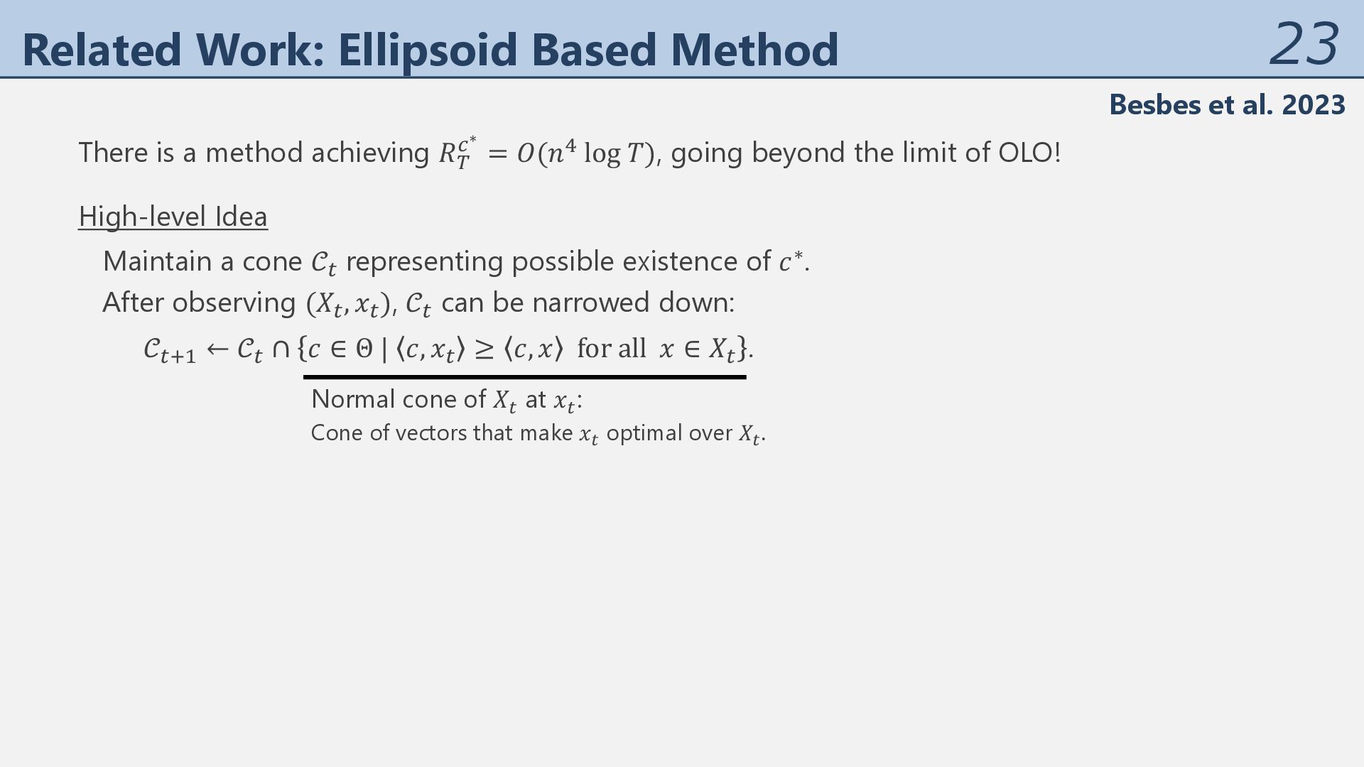
achieving 𝑅( -∗ = 𝑂(𝑛. log 𝑇), going beyond the limit of OLO! Besbes et al. 2023 High-level Idea Maintain a cone 𝒞% representing possible existence of 𝑐∗. After observing (𝑋%, 𝑥%), 𝒞% can be narrowed down: 𝒞%,' ← 𝒞% ∩ 𝑐 ∈ Θ | 𝑐, 𝑥% ≥ 𝑐, 𝑥 for all 𝑥 ∈ 𝑋% . Normal cone of 𝑋! at 𝑥! : Cone of vectors that make 𝑥! optimal over 𝑋! .
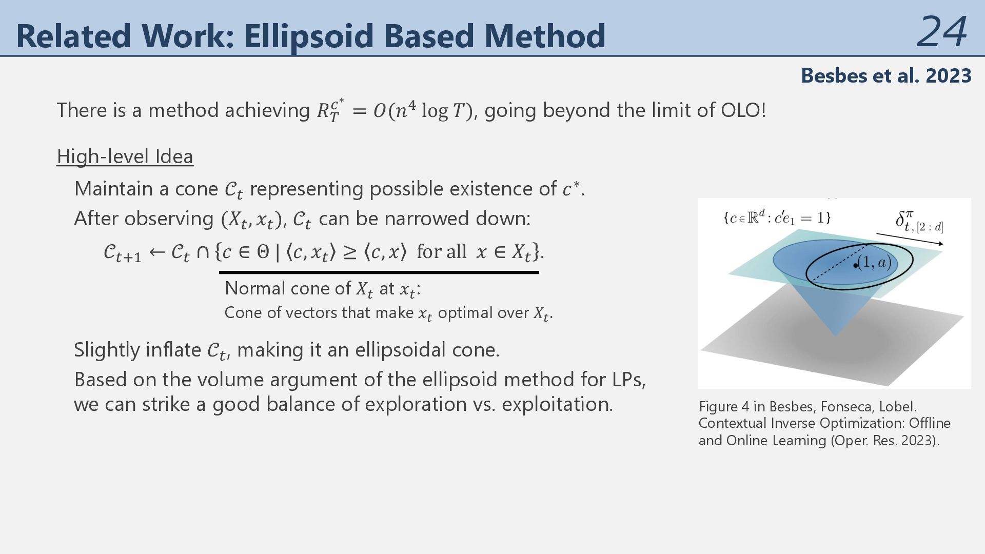
achieving 𝑅( -∗ = 𝑂(𝑛. log 𝑇), going beyond the limit of OLO! Besbes et al. 2023 Figure 4 in Besbes, Fonseca, Lobel. Contextual Inverse Optimization: Offline and Online Learning (Oper. Res. 2023). High-level Idea Maintain a cone 𝒞% representing possible existence of 𝑐∗. After observing (𝑋%, 𝑥%), 𝒞% can be narrowed down: 𝒞%,' ← 𝒞% ∩ 𝑐 ∈ Θ | 𝑐, 𝑥% ≥ 𝑐, 𝑥 for all 𝑥 ∈ 𝑋% . Normal cone of 𝑋! at 𝑥! : Cone of vectors that make 𝑥! optimal over 𝑋! . Slightly inflate 𝒞% , making it an ellipsoidal cone. Based on the volume argument of the ellipsoid method for LPs, we can strike a good balance of exploration vs. exploitation.
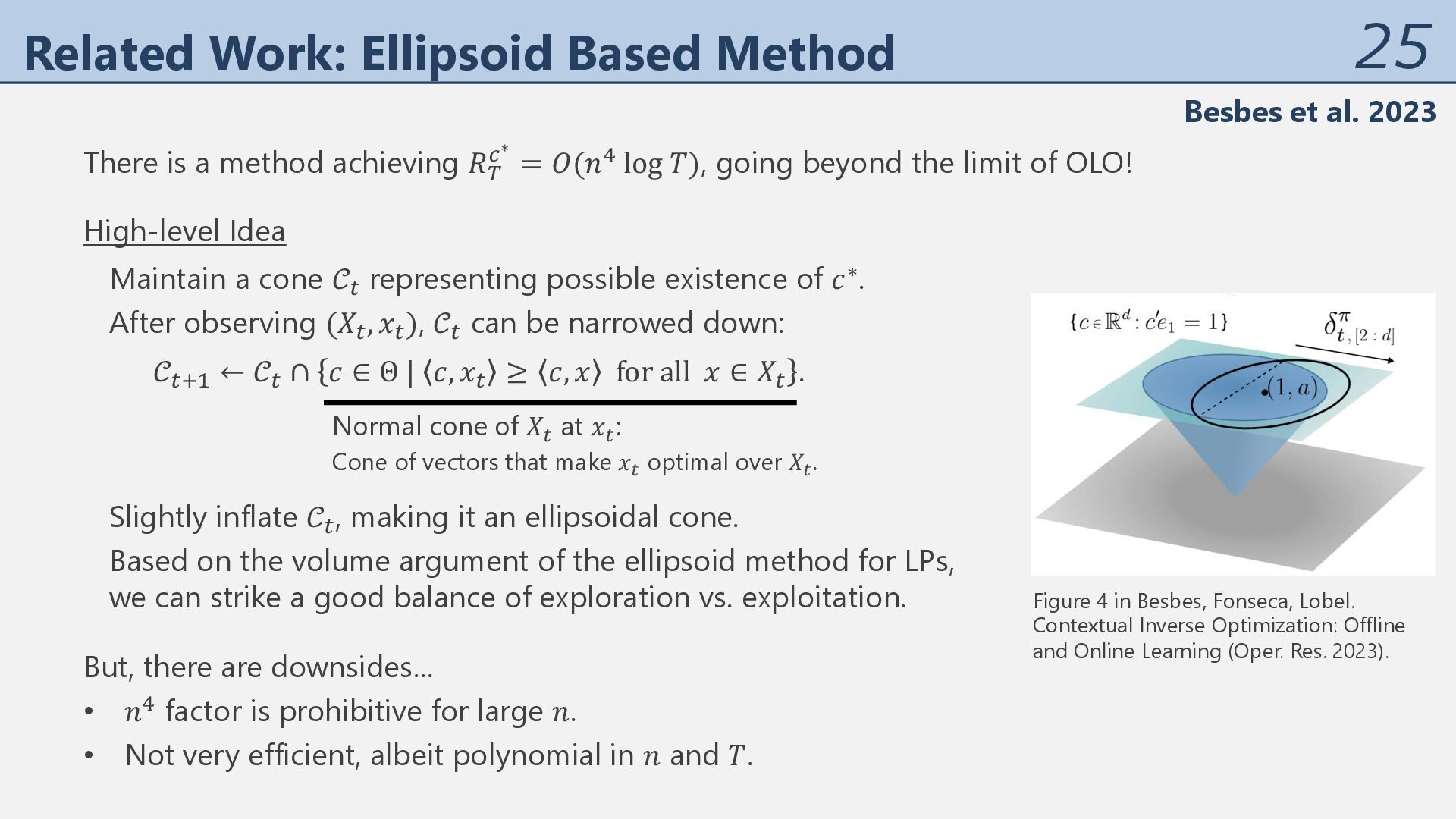
achieving 𝑅( -∗ = 𝑂(𝑛. log 𝑇), going beyond the limit of OLO! Besbes et al. 2023 Figure 4 in Besbes, Fonseca, Lobel. Contextual Inverse Optimization: Offline and Online Learning (Oper. Res. 2023). High-level Idea Maintain a cone 𝒞% representing possible existence of 𝑐∗. After observing (𝑋%, 𝑥%), 𝒞% can be narrowed down: 𝒞%,' ← 𝒞% ∩ 𝑐 ∈ Θ | 𝑐, 𝑥% ≥ 𝑐, 𝑥 for all 𝑥 ∈ 𝑋% . Normal cone of 𝑋! at 𝑥! : Cone of vectors that make 𝑥! optimal over 𝑋! . But, there are downsides… • 𝑛. factor is prohibitive for large 𝑛. • Not very efficient, albeit polynomial in 𝑛 and 𝑇. Slightly inflate 𝒞% , making it an ellipsoidal cone. Based on the volume argument of the ellipsoid method for LPs, we can strike a good balance of exploration vs. exploitation.
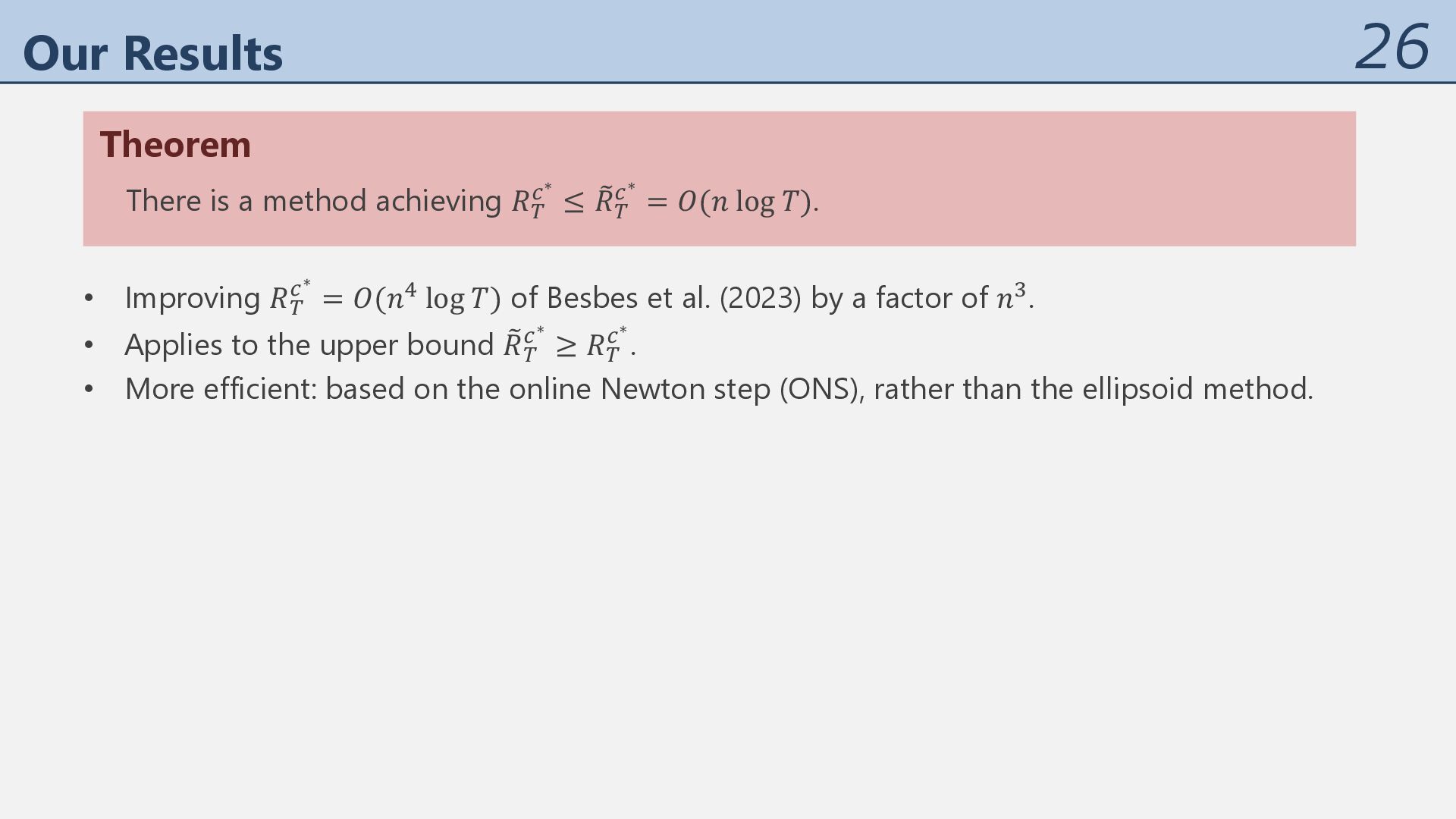
-∗ ≤ O 𝑅( -∗ = 𝑂(𝑛 log 𝑇). • Improving 𝑅( -∗ = 𝑂(𝑛. log 𝑇) of Besbes et al. (2023) by a factor of 𝑛/. • Applies to the upper bound O 𝑅( -∗ ≥ 𝑅( -∗ . • More efficient: based on the online Newton step (ONS), rather than the ellipsoid method.
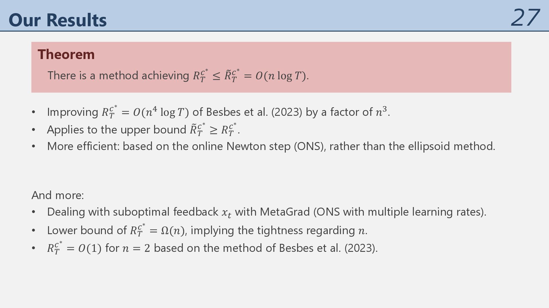
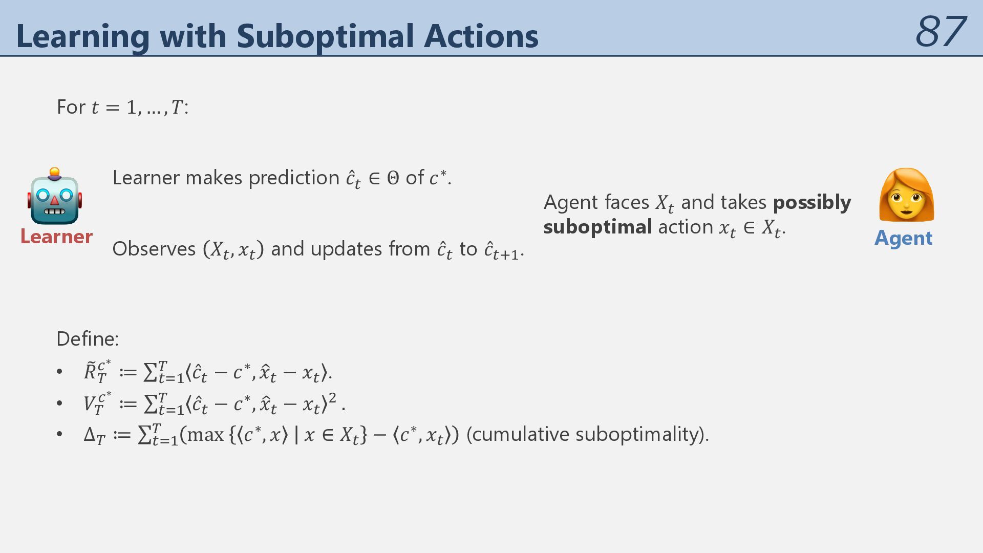
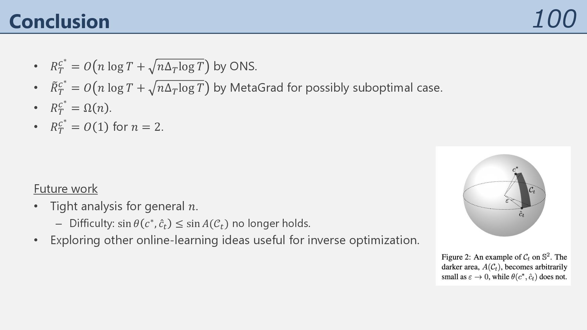
-∗ ≤ O 𝑅( -∗ = 𝑂(𝑛 log 𝑇). And more: • Dealing with suboptimal feedback 𝑥% with MetaGrad (ONS with multiple learning rates). • Lower bound of 𝑅( -∗ = Ω(𝑛), implying the tightness regarding 𝑛. • 𝑅( -∗ = 𝑂(1) for 𝑛 = 2 based on the method of Besbes et al. (2023). • Improving 𝑅( -∗ = 𝑂(𝑛. log 𝑇) of Besbes et al. (2023) by a factor of 𝑛/. • Applies to the upper bound O 𝑅( -∗ ≥ 𝑅( -∗ . • More efficient: based on the online Newton step (ONS), rather than the ellipsoid method.
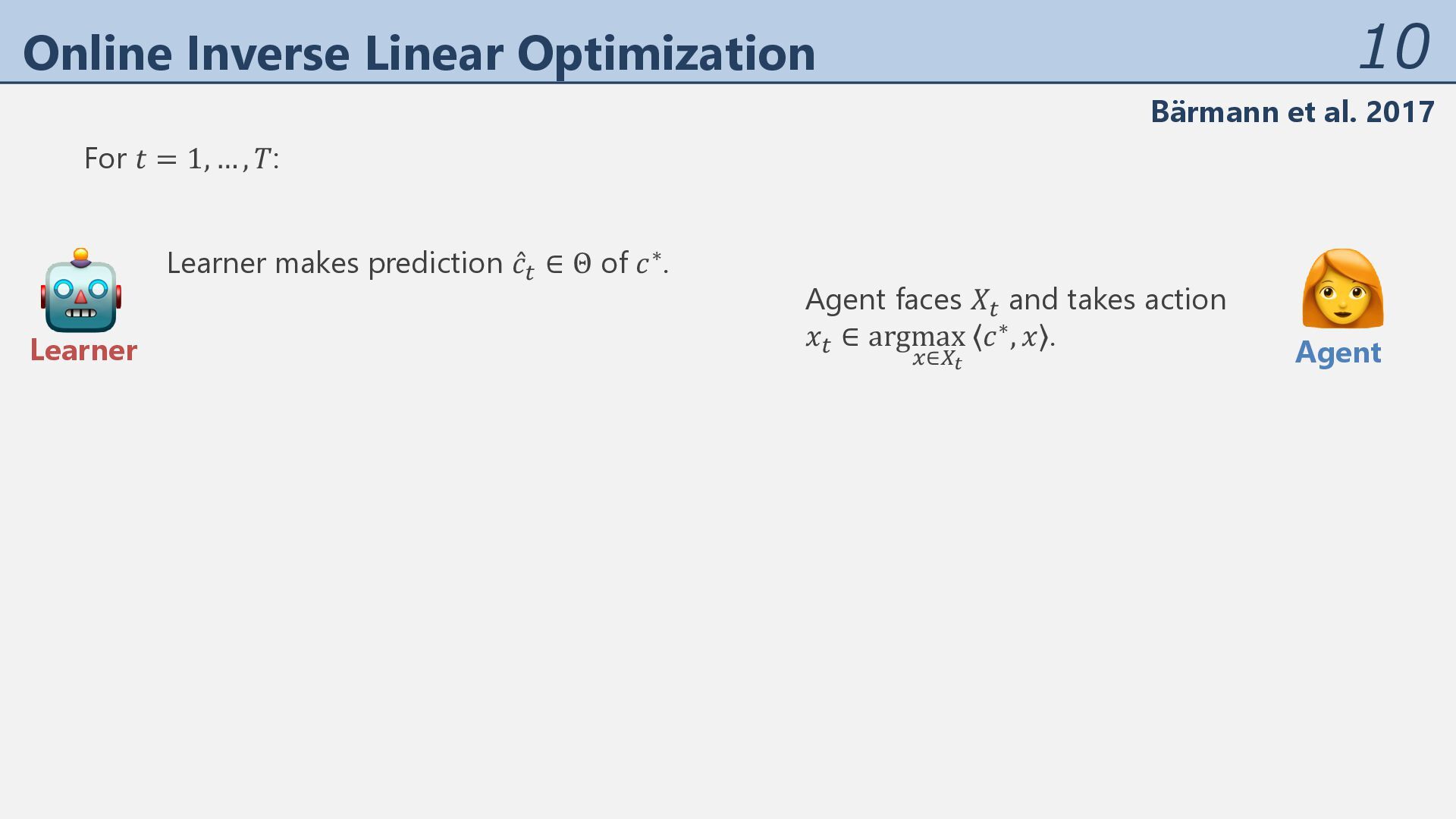
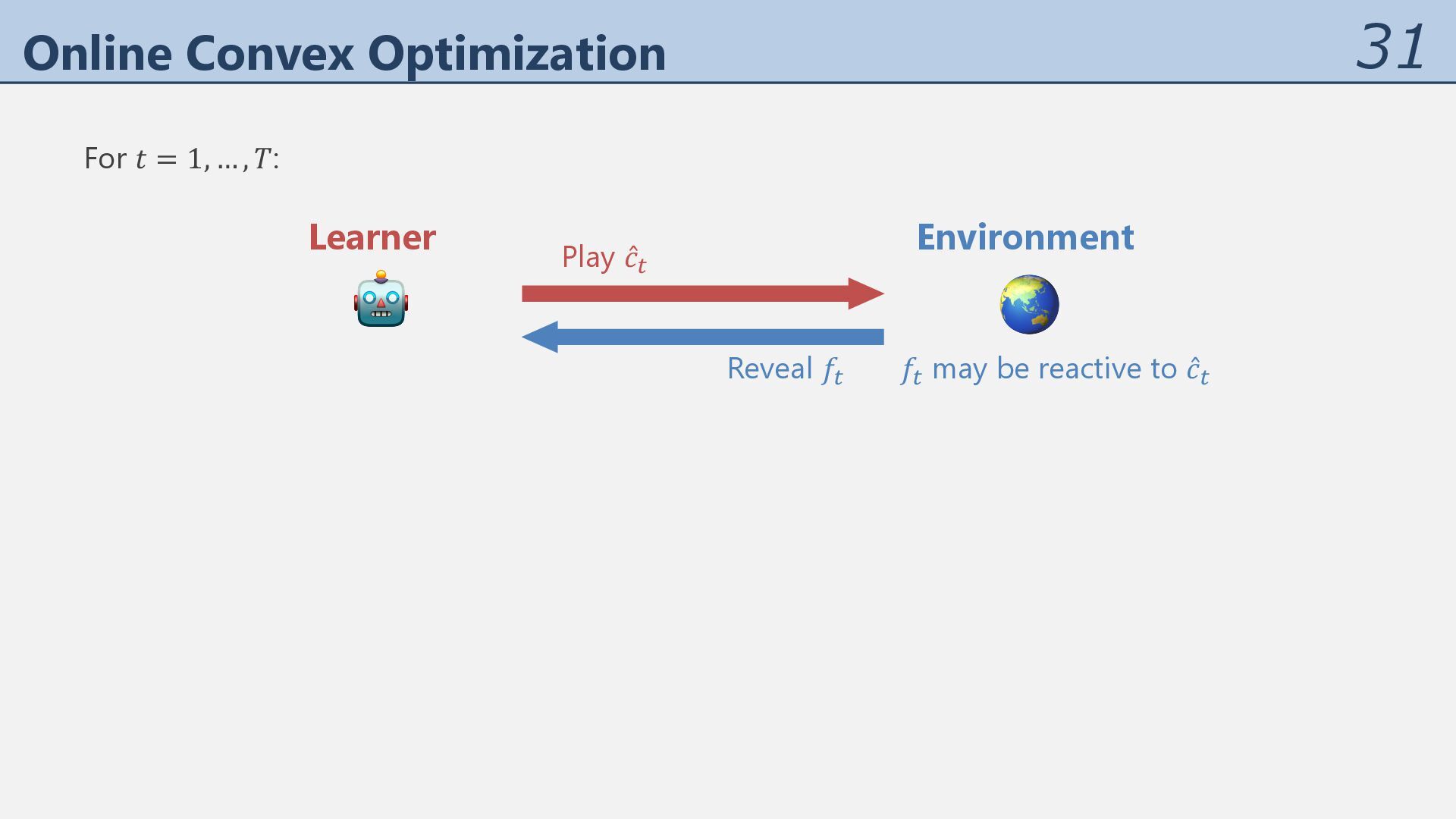
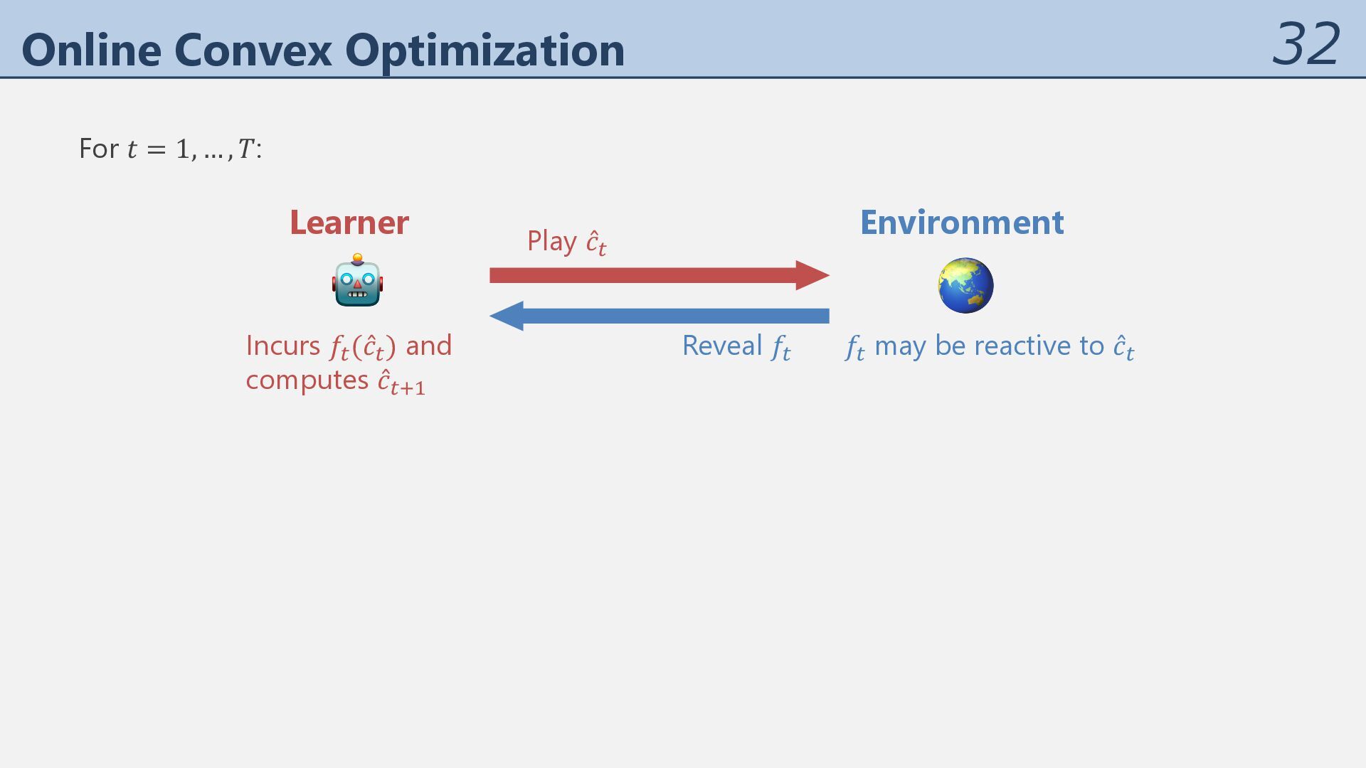
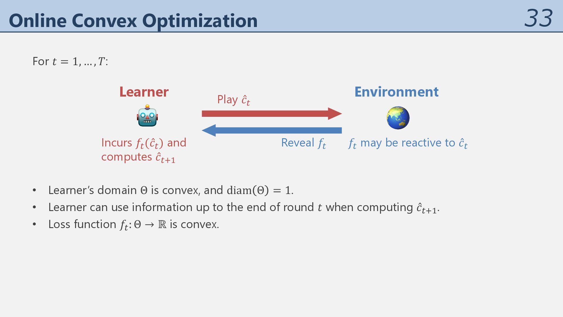
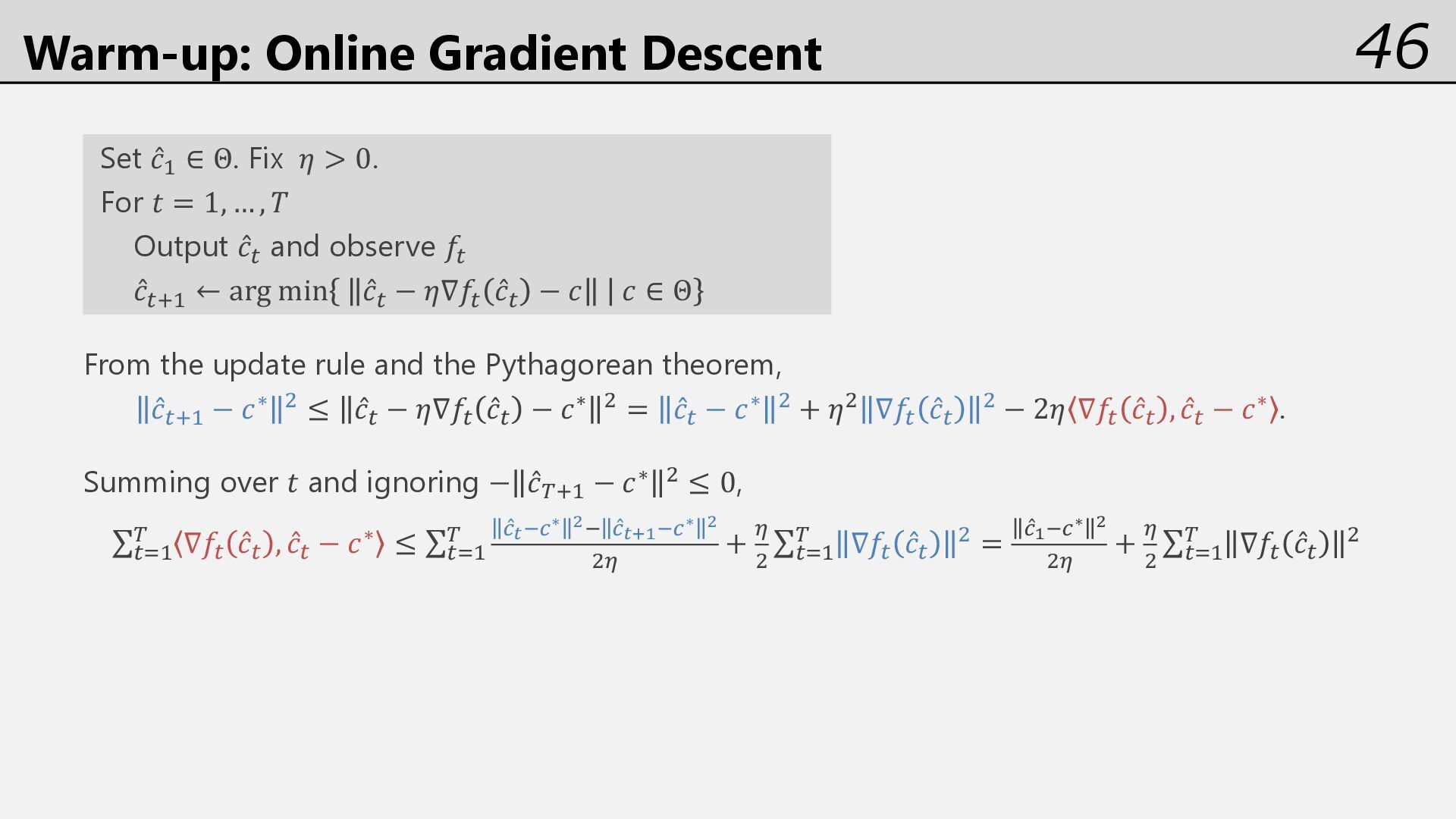
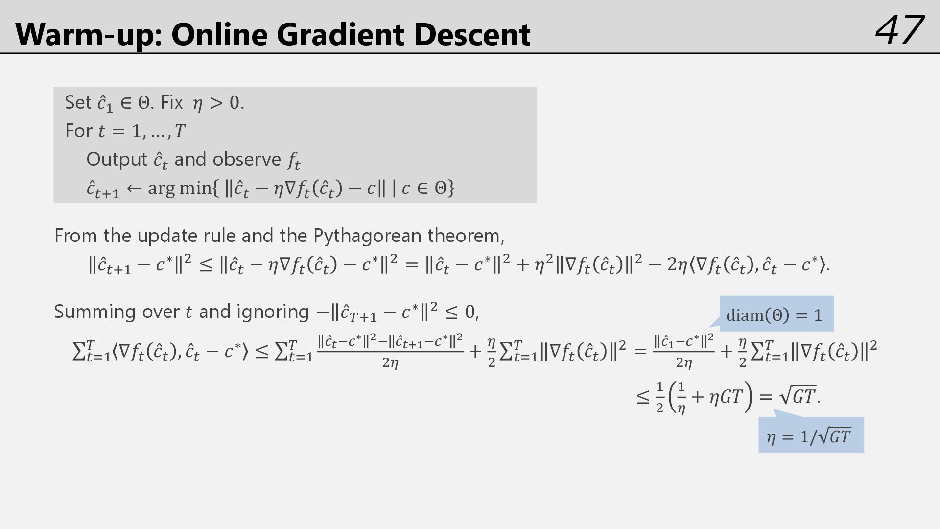
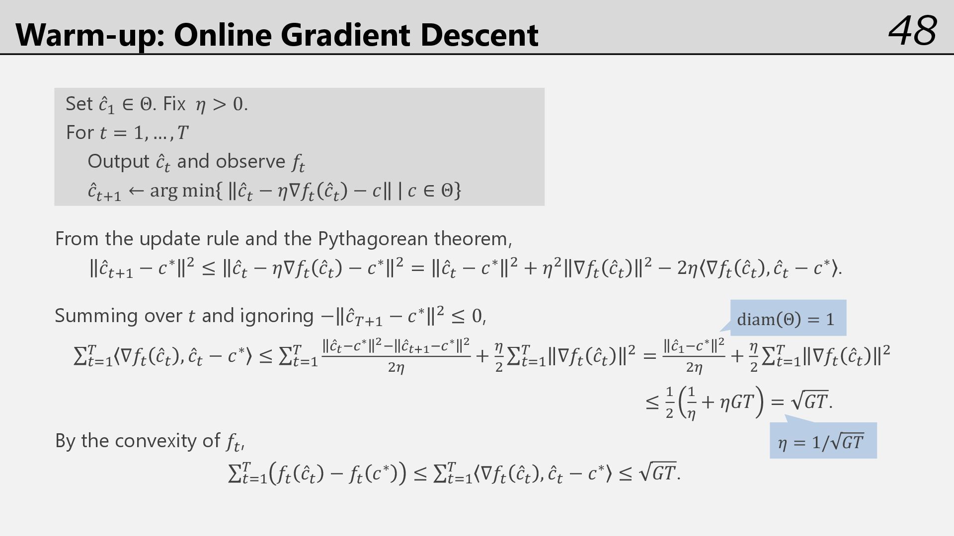
and diam Θ = 1. • Learner can use information up to the end of round 𝑡 when computing ̂ 𝑐%,' . • Loss function 𝑓%: Θ → ℝ is convex. For 𝑡 = 1, … , 𝑇: Reveal 𝑓% Play ̂ 𝑐% 🤖 🌏 Learner Environment 𝑓% may be reactive to ̂ 𝑐% Incurs 𝑓%( ̂ 𝑐%) and computes ̂ 𝑐%,'
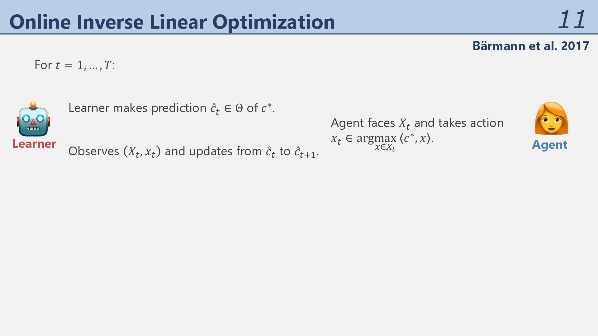
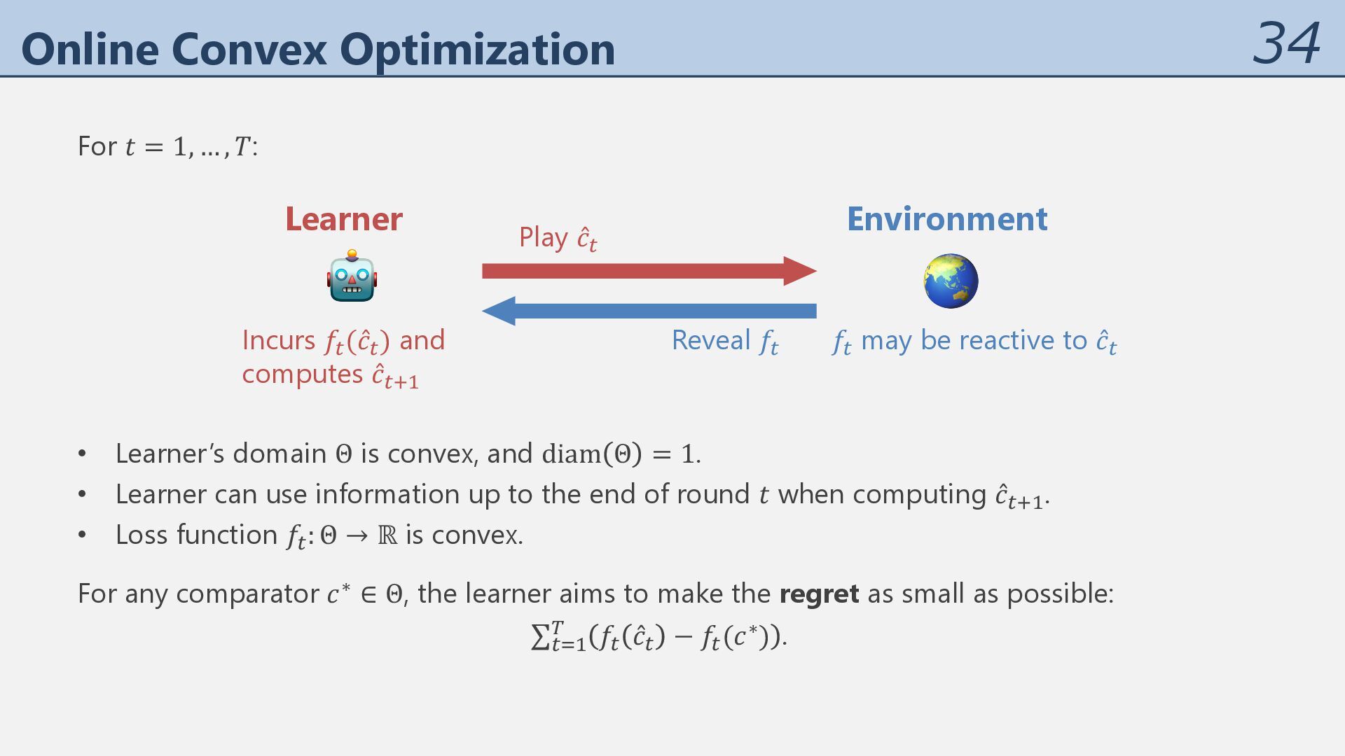
𝑇: Reveal 𝑓% Play ̂ 𝑐% 🤖 🌏 Learner Environment 𝑓% may be reactive to ̂ 𝑐% For any comparator 𝑐∗ ∈ Θ, the learner aims to make the regret as small as possible: ∑%&' ( 𝑓% ̂ 𝑐% − 𝑓%(𝑐∗) . • Learner’s domain Θ is convex, and diam Θ = 1. • Learner can use information up to the end of round 𝑡 when computing ̂ 𝑐%,' . • Loss function 𝑓%: Θ → ℝ is convex. Incurs 𝑓%( ̂ 𝑐%) and computes ̂ 𝑐%,'
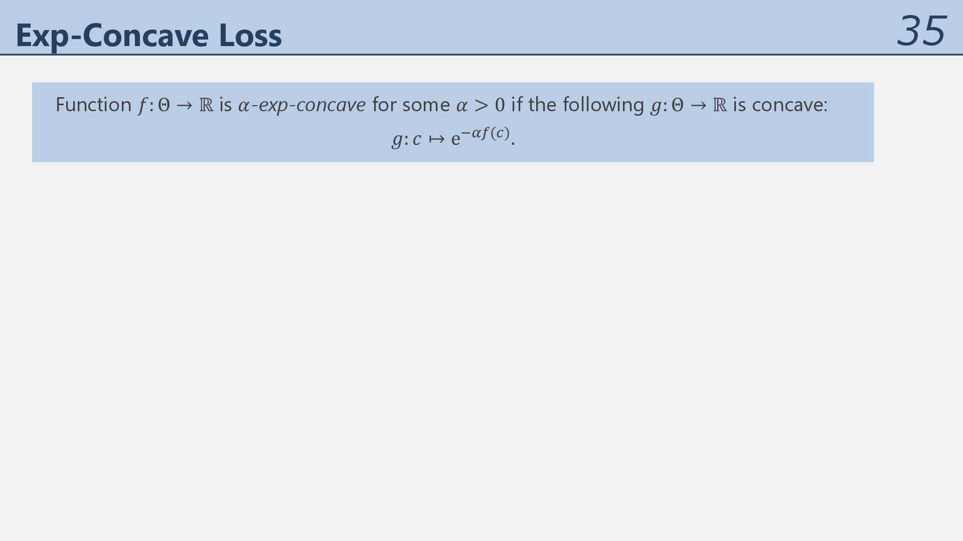
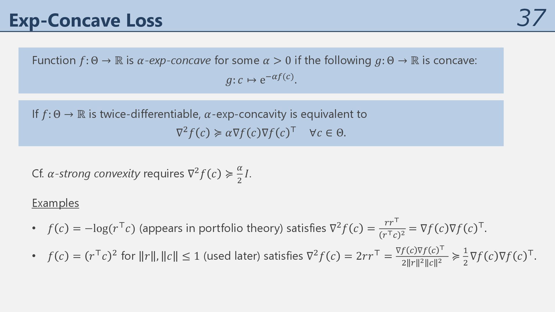
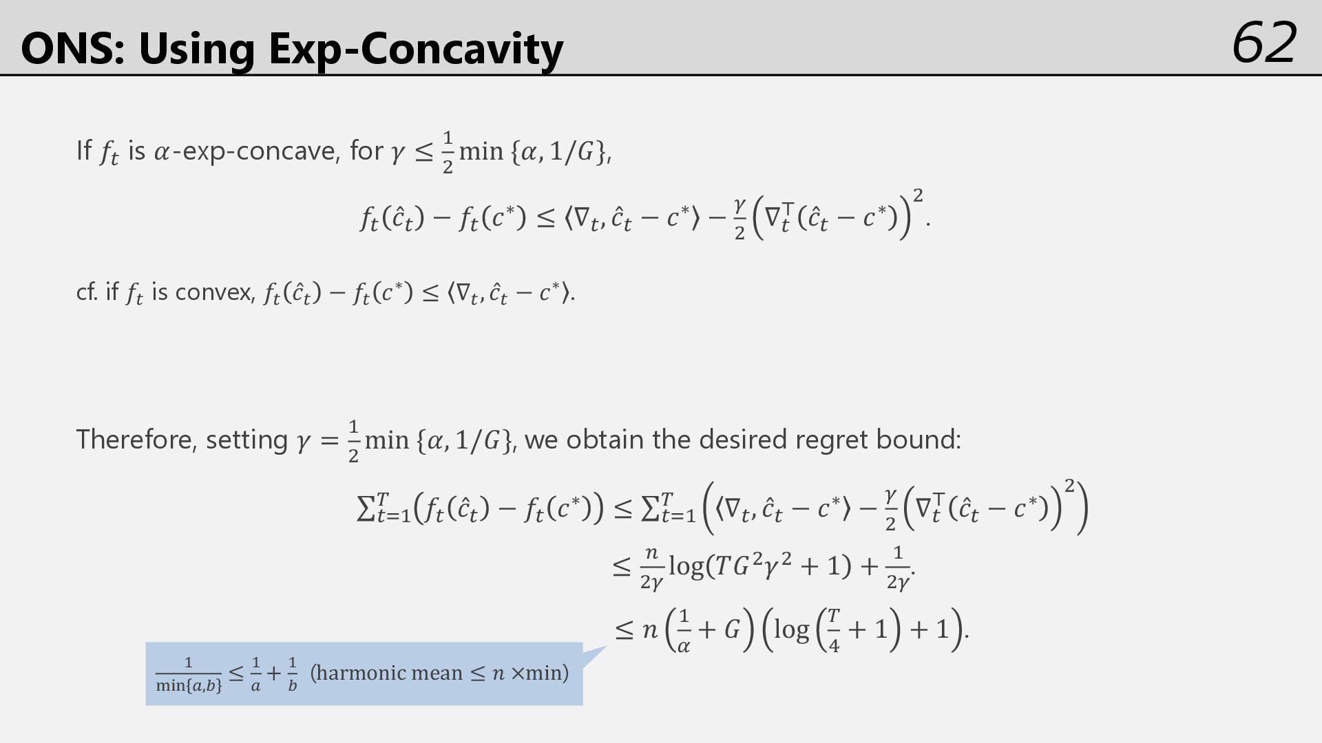
for some 𝛼 > 0 if the following 𝑔: Θ → ℝ is concave: 𝑔: 𝑐 ↦ e012(-). If 𝑓: Θ → ℝ is twice-differentiable, 𝛼-exp-concavity is equivalent to ∇5𝑓 𝑐 ≽ 𝛼∇𝑓 𝑐 ∇𝑓 𝑐 6 ∀𝑐 ∈ Θ. Cf. 𝛼-strong convexity requires ∇5𝑓 𝑐 ≽ 1 5 𝐼.
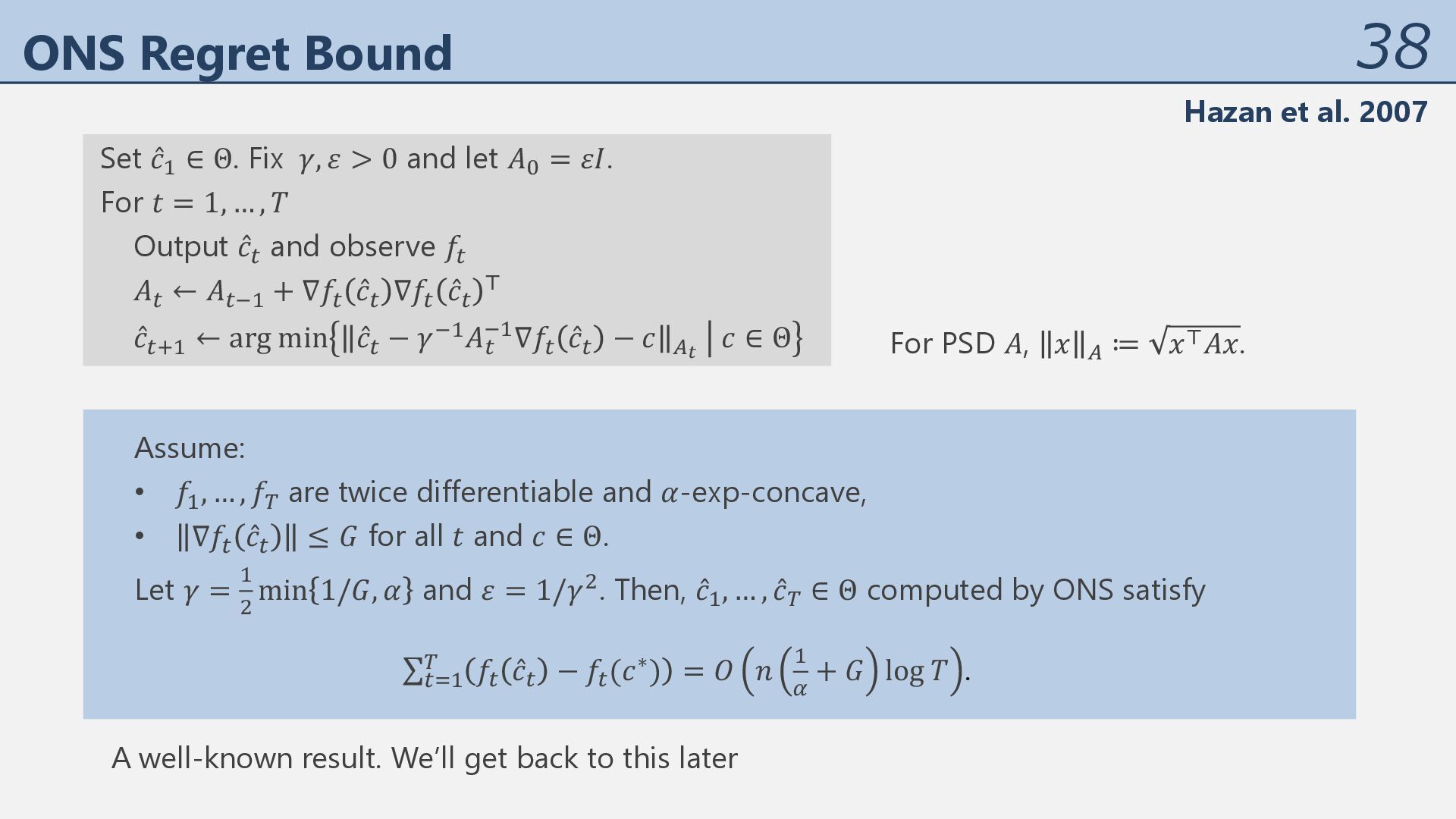
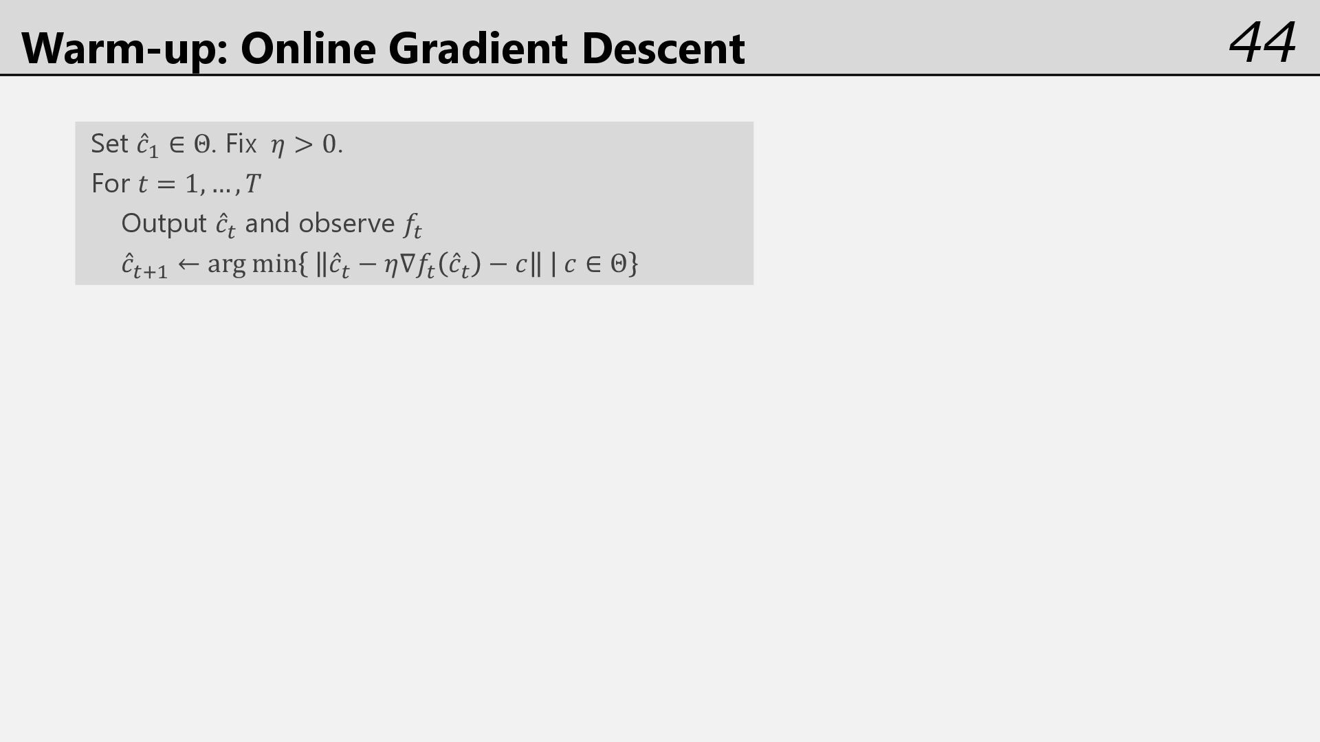
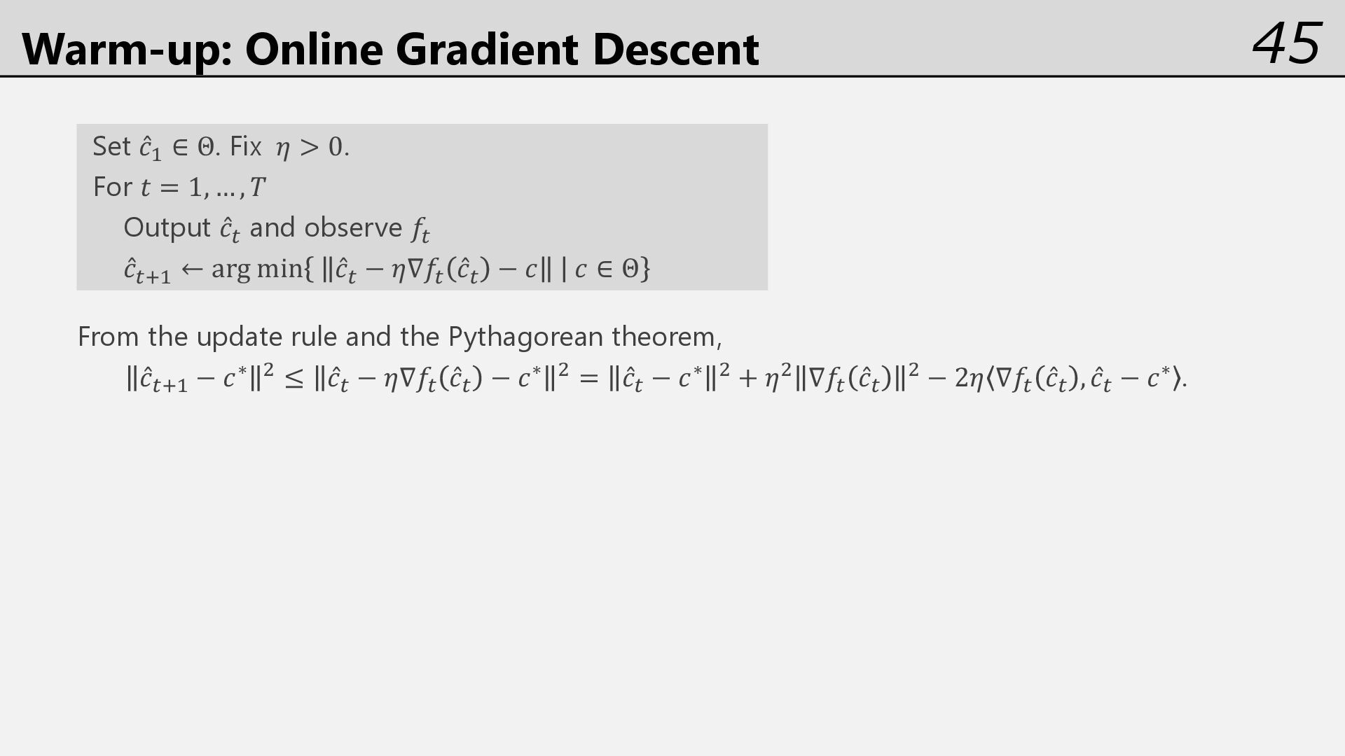
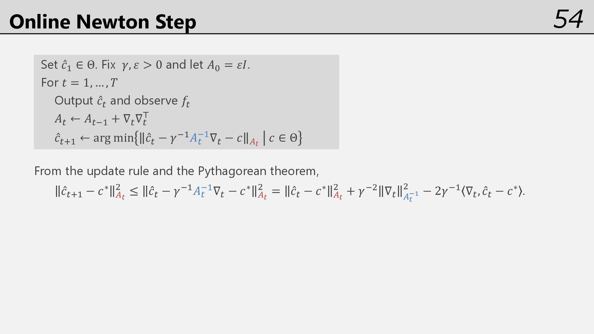
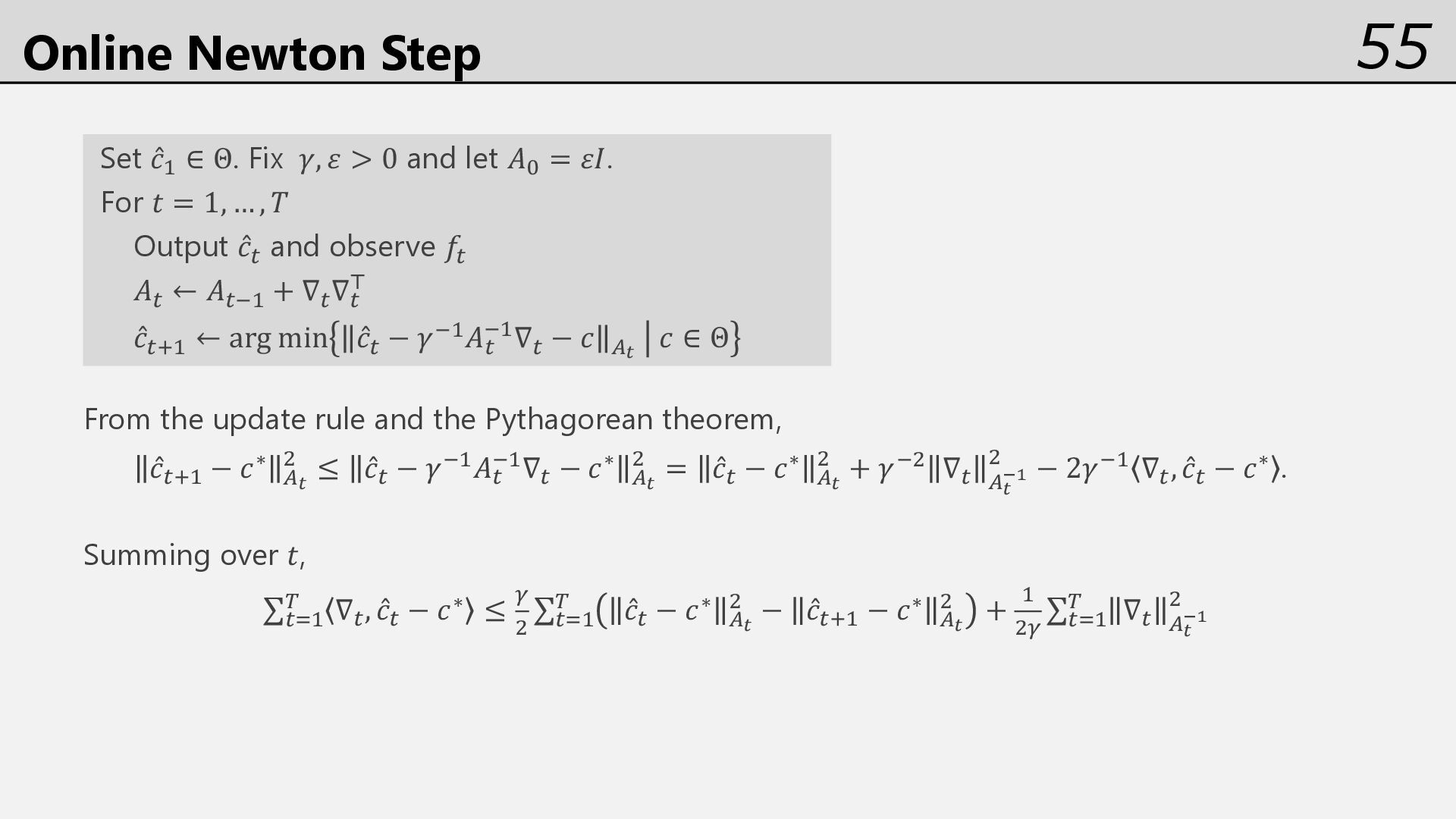
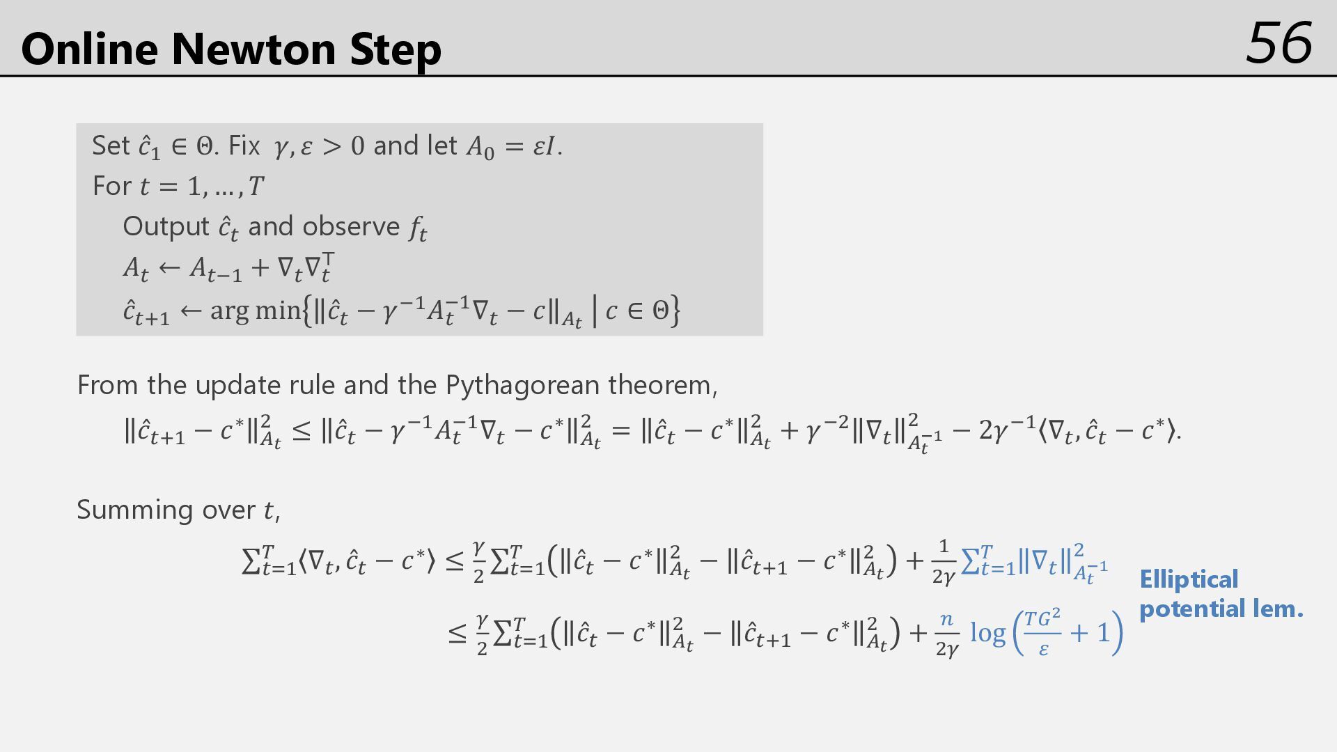
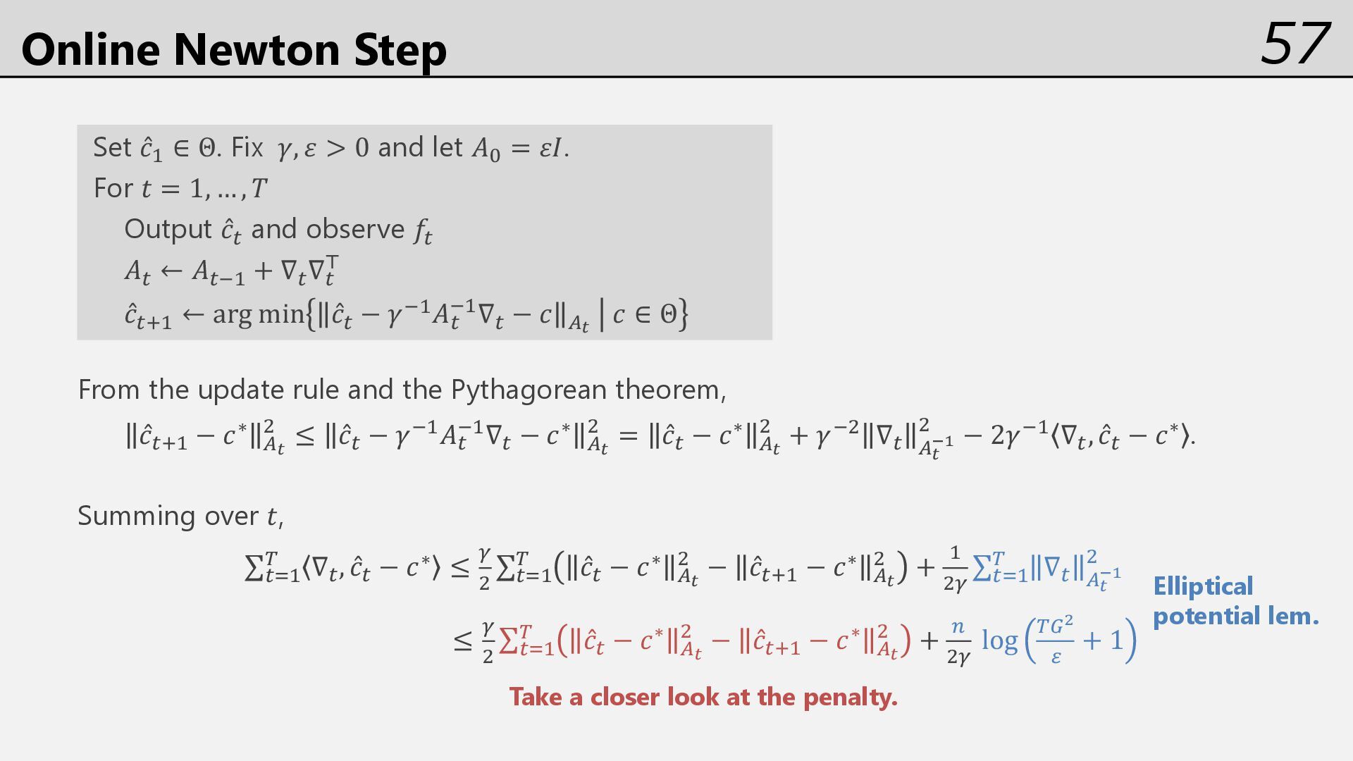
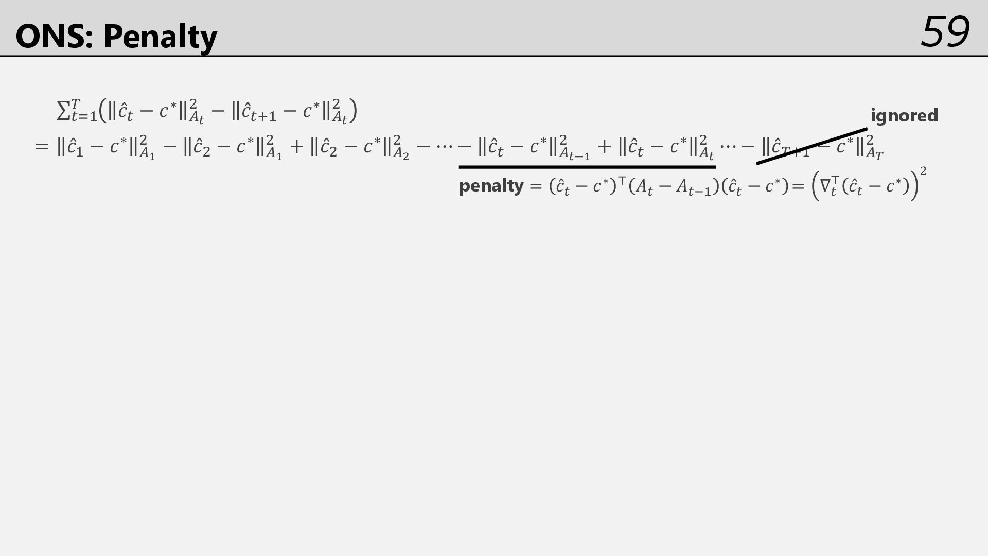
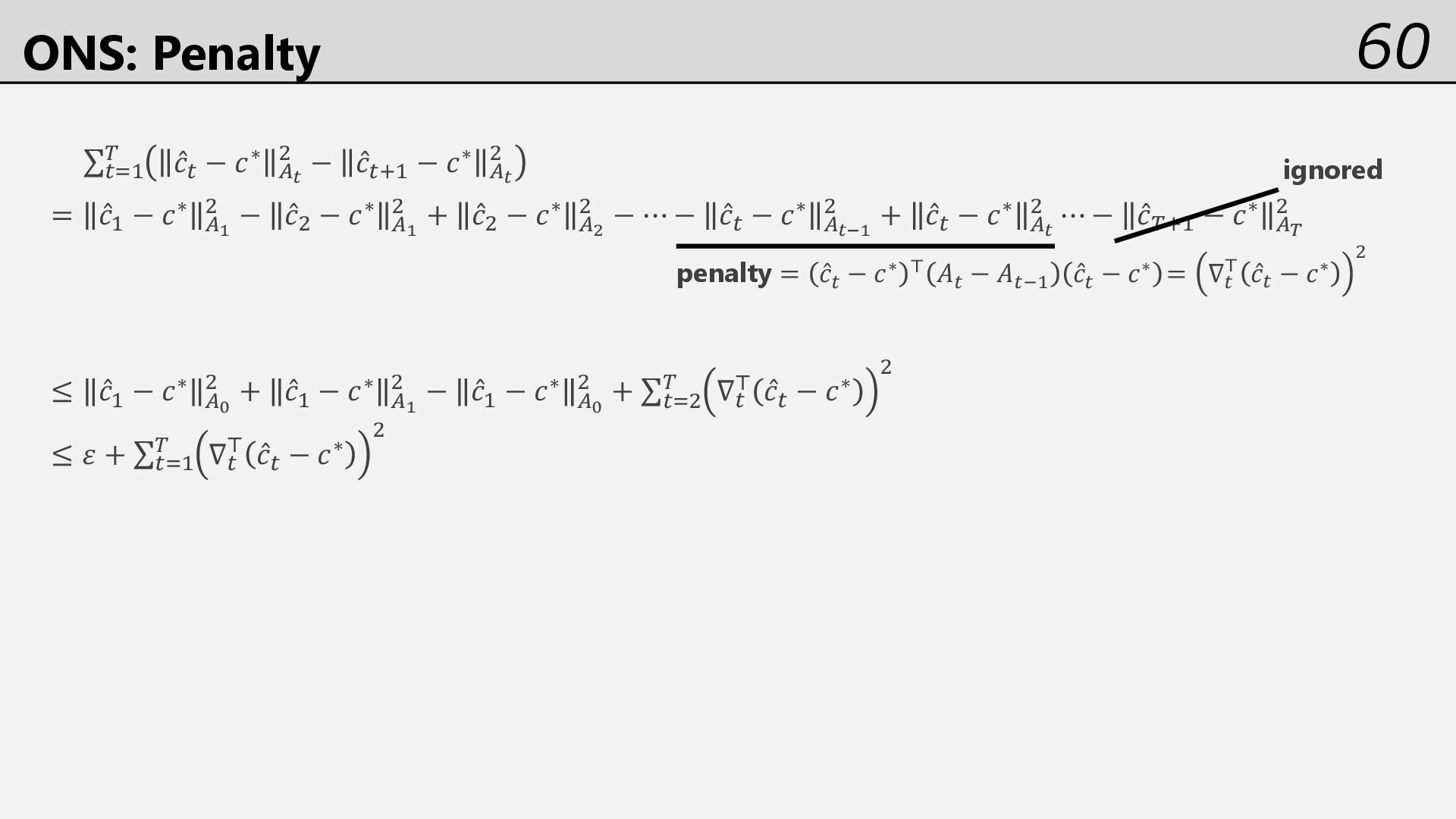
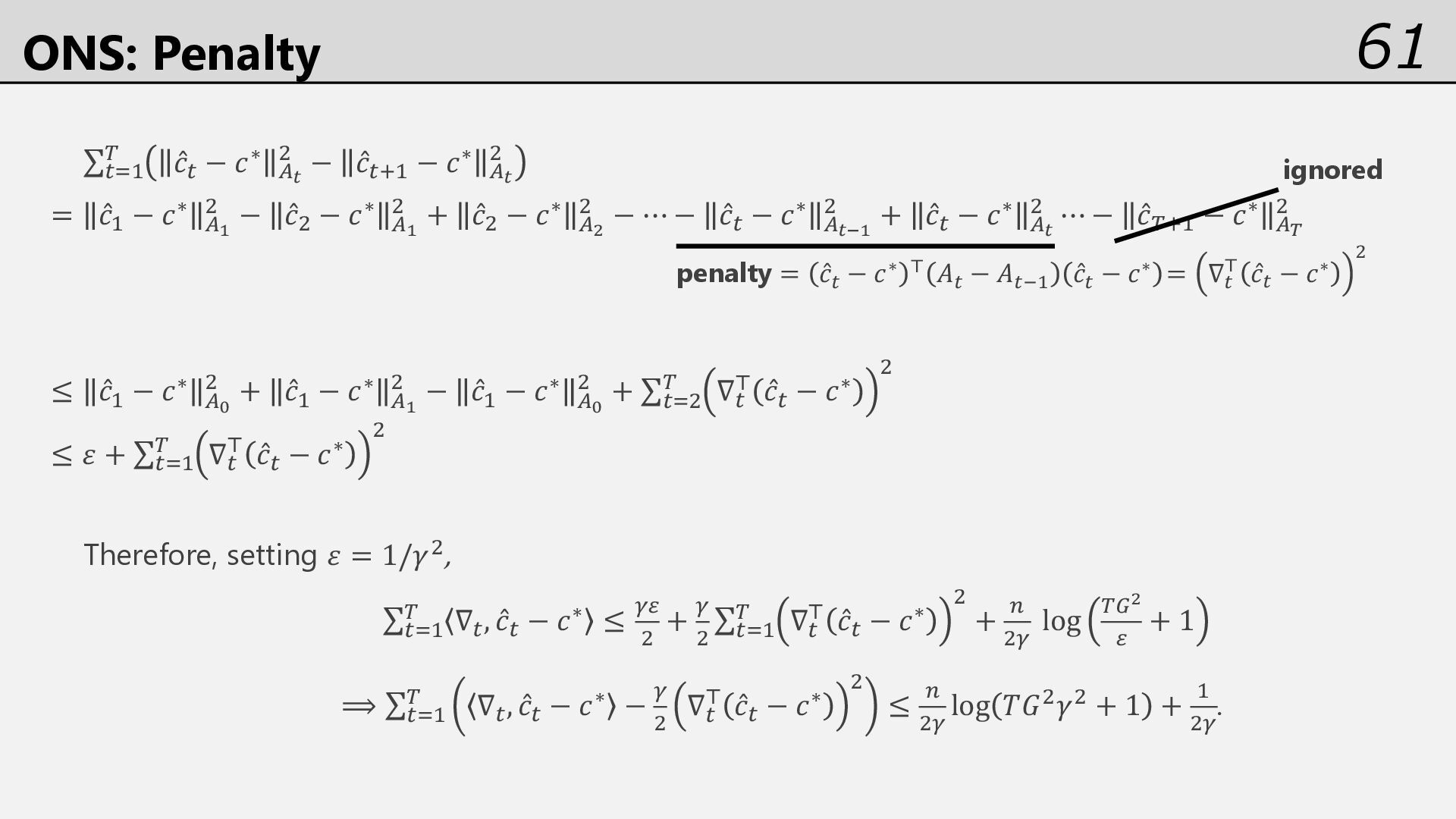
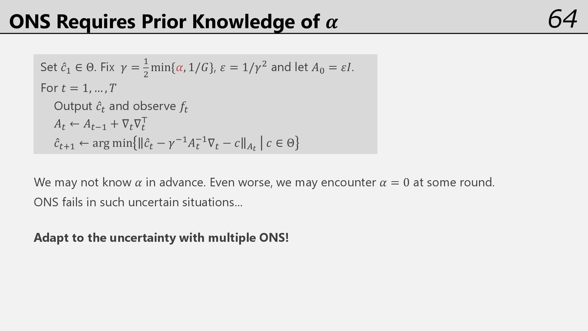
∈ Θ. Fix 𝛾 = ' 5 min{𝛼, 1/𝐺}, 𝜀 = 1/𝛾5 and let 𝐴9 = 𝜀𝐼. For 𝑡 = 1, … , 𝑇 Output ̂ 𝑐% and observe 𝑓% 𝐴% ← 𝐴%0' + ∇%∇% 6 ̂ 𝑐%,' ← arg min ̂ 𝑐% − 𝛾0'𝐴% 0'∇% − 𝑐 :" 𝑐 ∈ Θ We may not know 𝛼 in advance. Even worse, we may encounter 𝛼 = 0 at some round. ONS fails in such uncertain situations… Adapt to the uncertainty with multiple ONS!
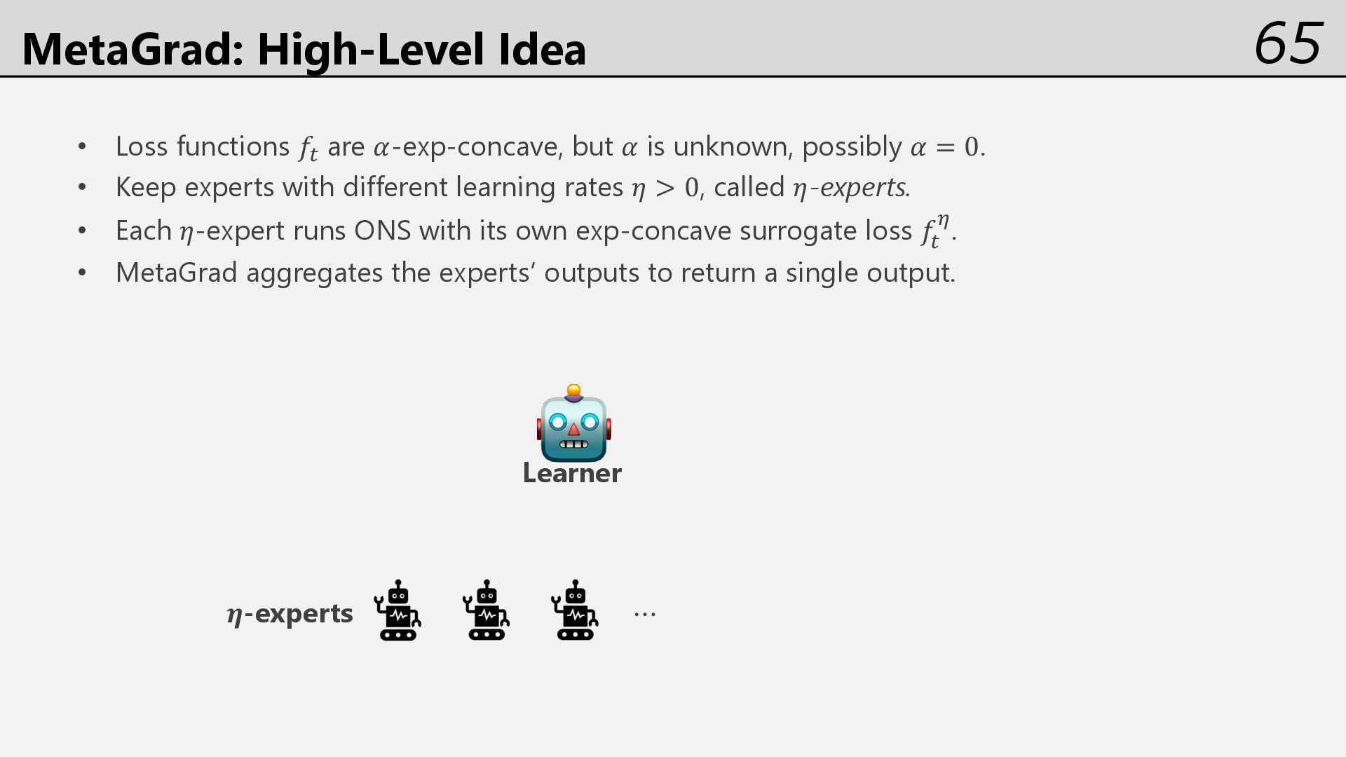
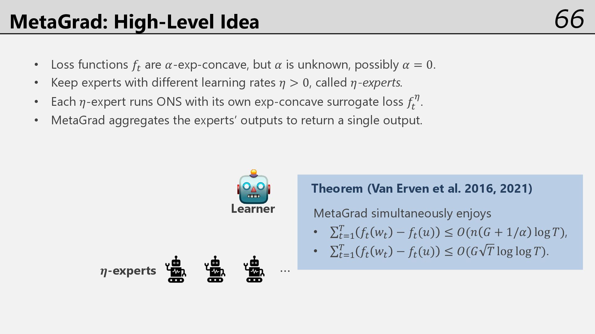
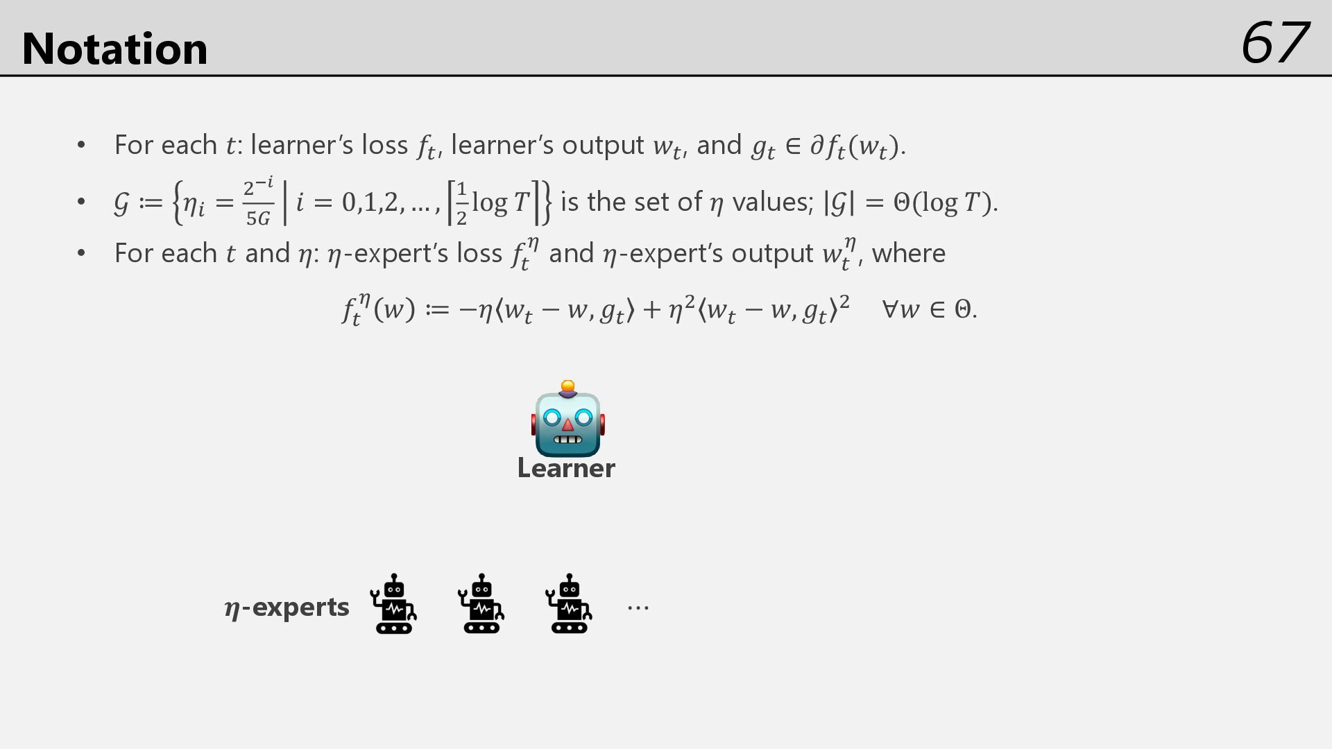
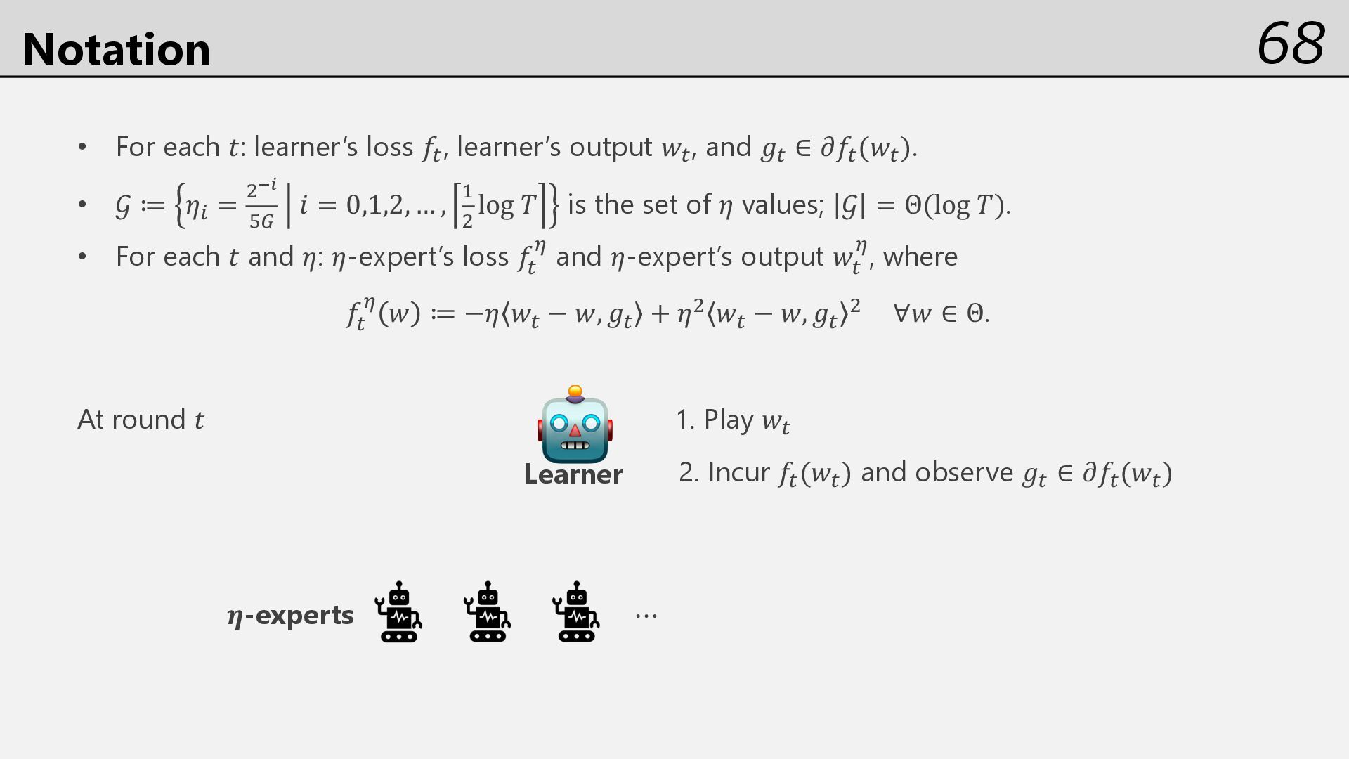
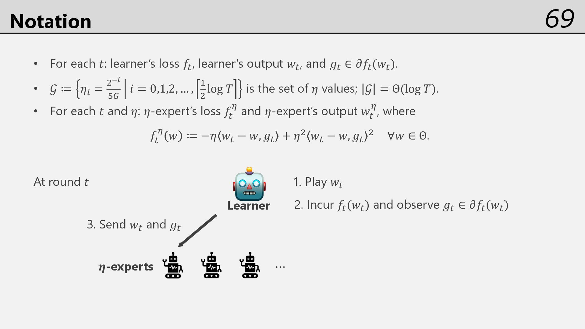
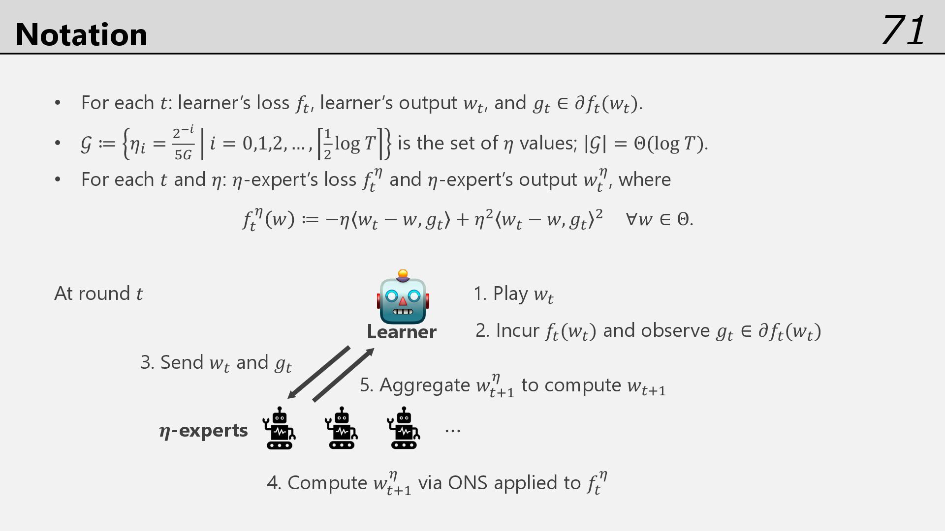
but 𝛼 is unknown, possibly 𝛼 = 0. • Keep experts with different learning rates 𝜂 > 0, called 𝜂-experts. • Each 𝜂-expert runs ONS with its own exp-concave surrogate loss 𝑓% ;. • MetaGrad aggregates the experts’ outputs to return a single output. ⋯ 𝜼-experts 🤖 Learner
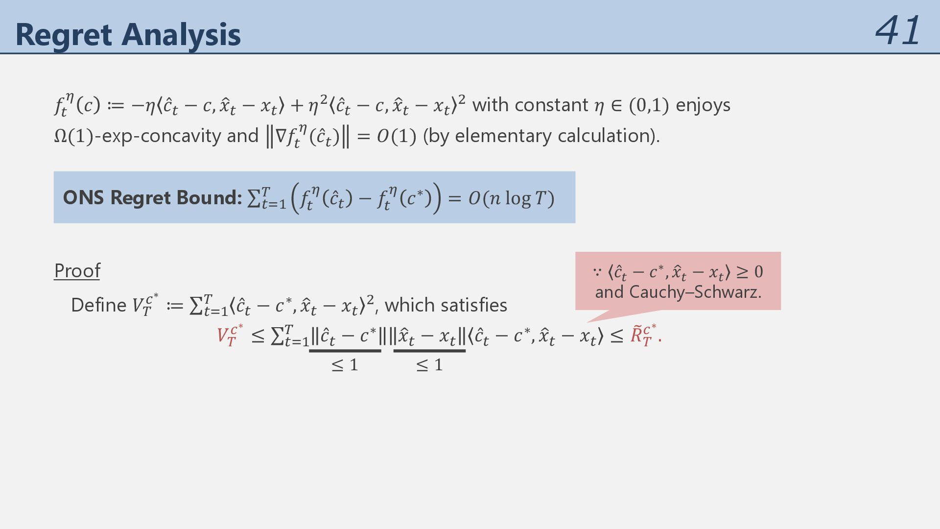
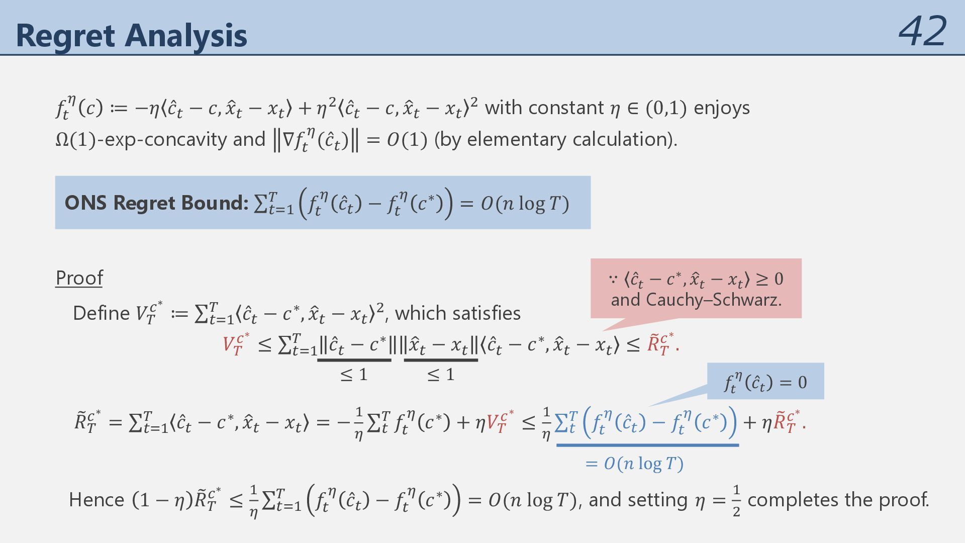
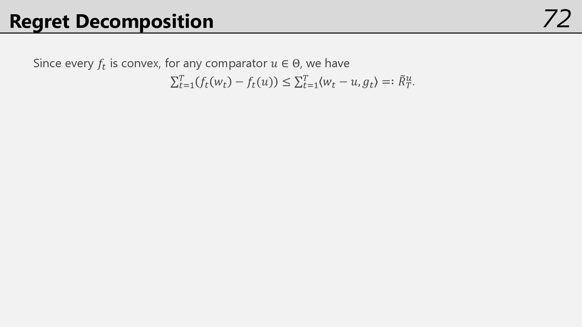
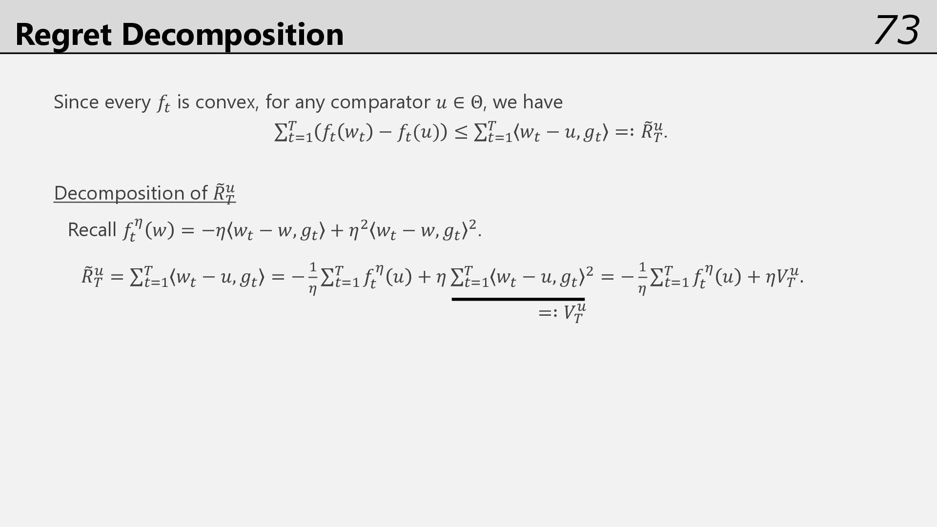
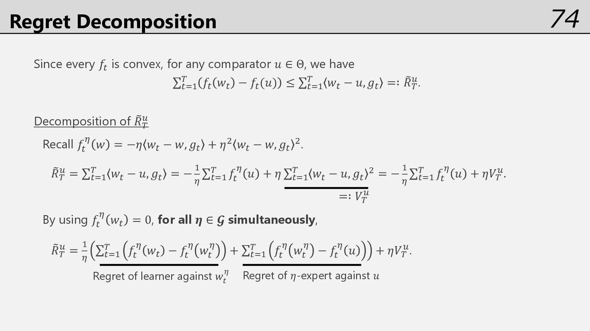
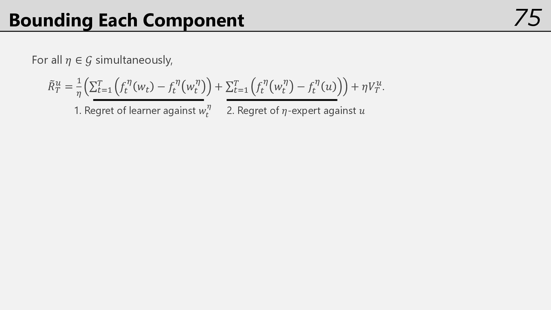
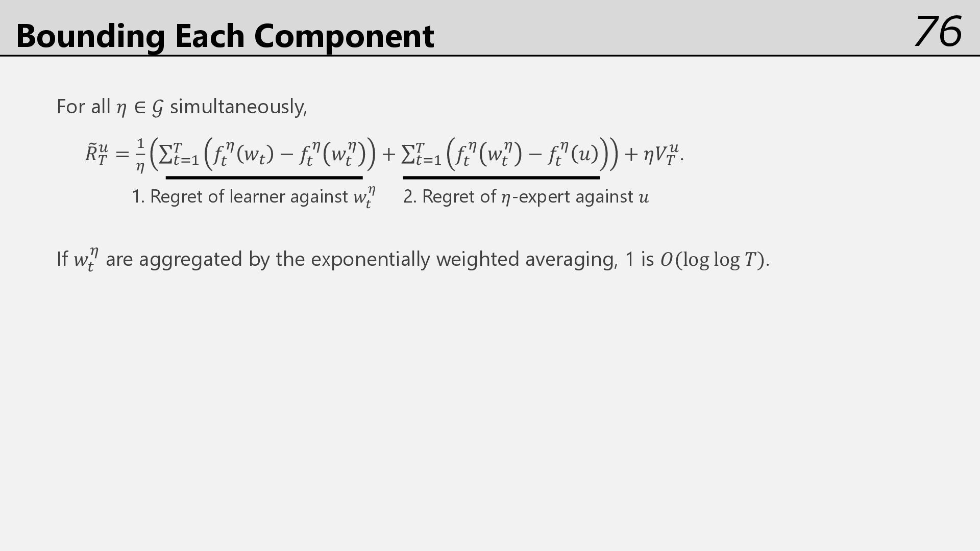
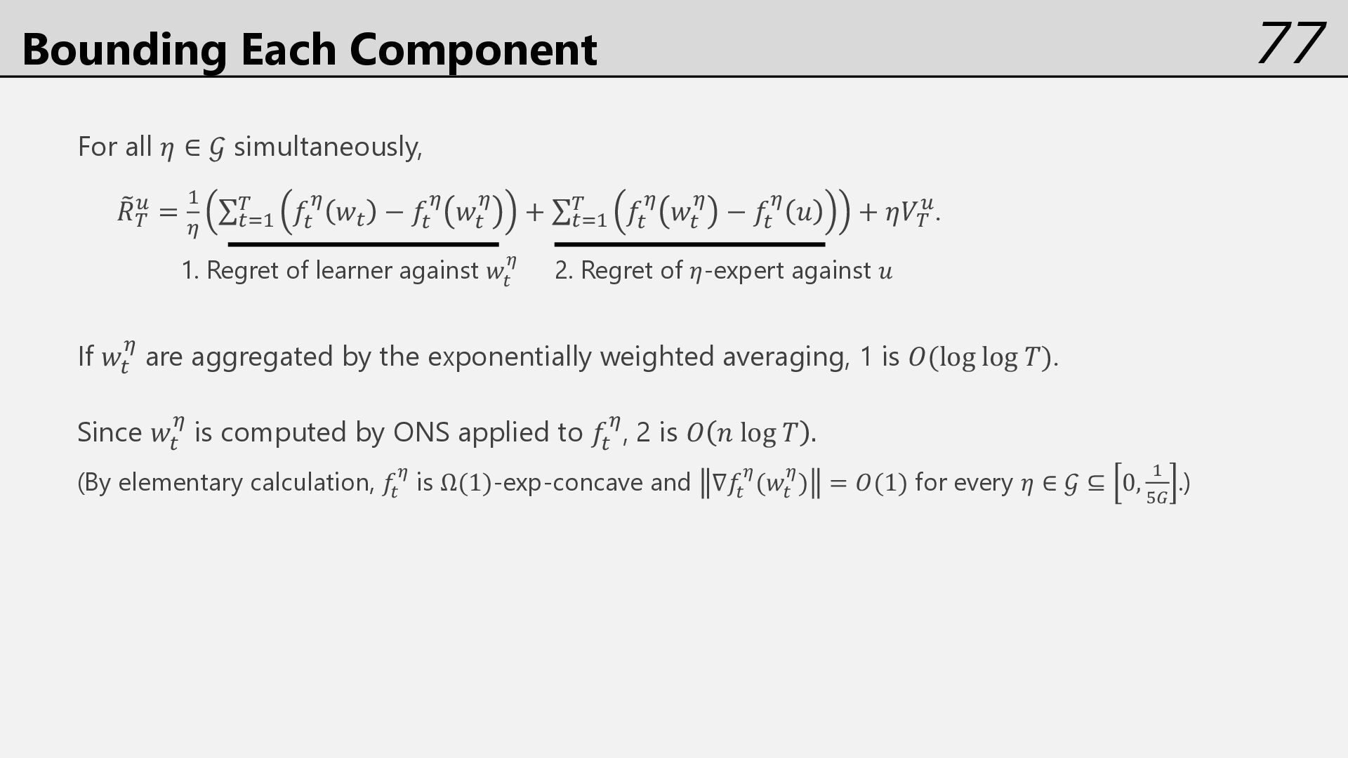
O 𝑅( E = ' ; ∑%&' ( 𝑓% ; 𝑤% − 𝑓% ; 𝑤% ; + ∑%&' ( 𝑓% ; 𝑤% ; − 𝑓% ; 𝑢 + 𝜂𝑉( E. If 𝑤% ; are aggregated by the exponentially weighted averaging, 1 is 𝑂(log log 𝑇). 1. Regret of learner against 𝑤! ' 2. Regret of 𝜂-expert against 𝑢
O 𝑅( E = ' ; ∑%&' ( 𝑓% ; 𝑤% − 𝑓% ; 𝑤% ; + ∑%&' ( 𝑓% ; 𝑤% ; − 𝑓% ; 𝑢 + 𝜂𝑉( E. If 𝑤% ; are aggregated by the exponentially weighted averaging, 1 is 𝑂(log log 𝑇). Since 𝑤% ; is computed by ONS applied to 𝑓% ;, 2 is 𝑂 𝑛 log 𝑇 . (By elementary calculation, 𝑓! ' is Ω(1)-exp-concave and ∇𝑓! '(𝑤! ') = 𝑂(1) for every 𝜂 ∈ 𝒢 ⊆ 0, % -. .) 1. Regret of learner against 𝑤! ' 2. Regret of 𝜂-expert against 𝑢
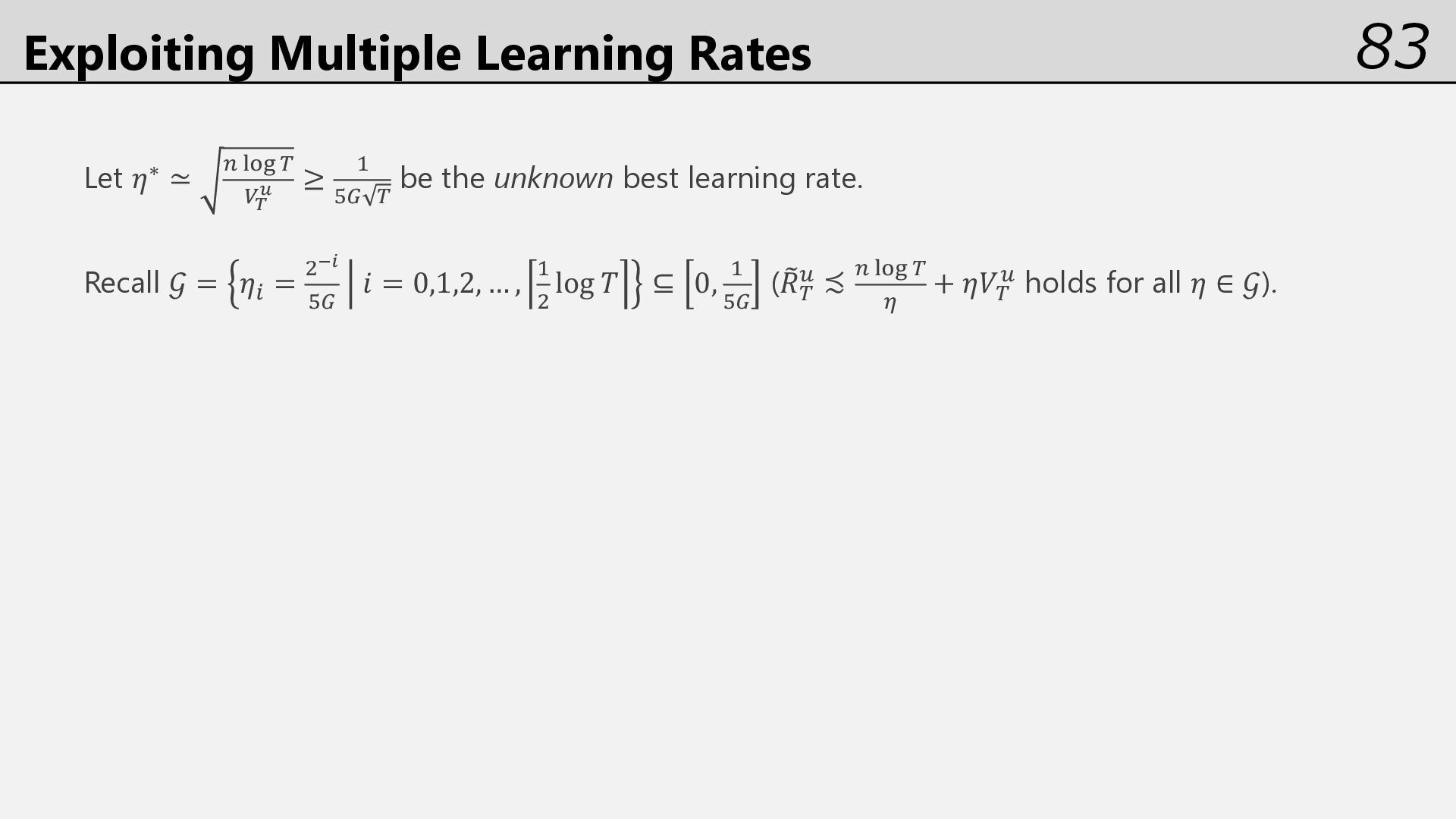
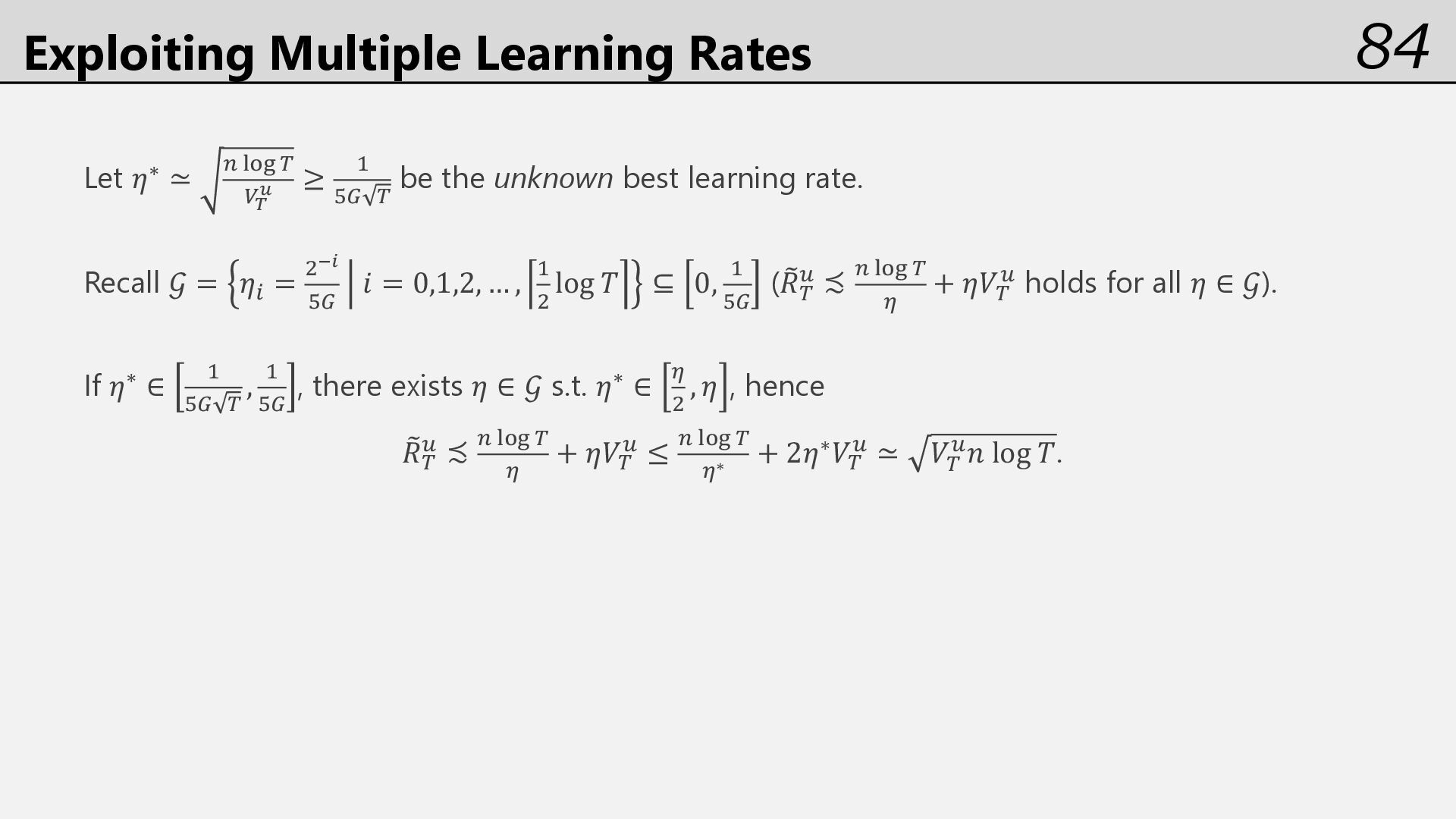
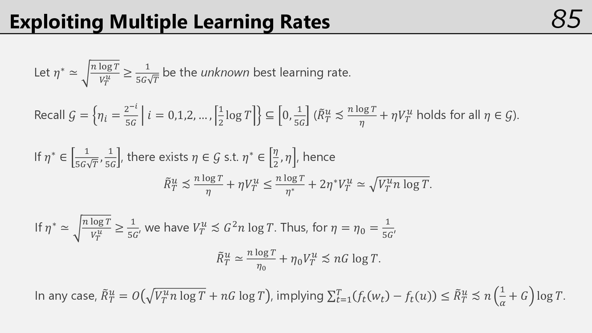
O 𝑅( E = ' ; ∑%&' ( 𝑓% ; 𝑤% − 𝑓% ; 𝑤% ; + ∑%&' ( 𝑓% ; 𝑤% ; − 𝑓% ; 𝑢 + 𝜂𝑉( E. If 𝑤% ; are aggregated by the exponentially weighted averaging, 1 is 𝑂(log log 𝑇). Since 𝑤% ; is computed by ONS applied to 𝑓% ;, 2 is 𝑂 𝑛 log 𝑇 . (By elementary calculation, 𝑓! ' is Ω(1)-exp-concave and ∇𝑓! '(𝑤! ') = 𝑂(1) for every 𝜂 ∈ 𝒢 ⊆ 0, % -. .) Therefore, for all 𝜂 ∈ 𝒢 simultaneously, O 𝑅( E = 𝑂 " FGH ( ; + 𝜂𝑉( E . 1. Regret of learner against 𝑤! ' 2. Regret of 𝜂-expert against 𝑢
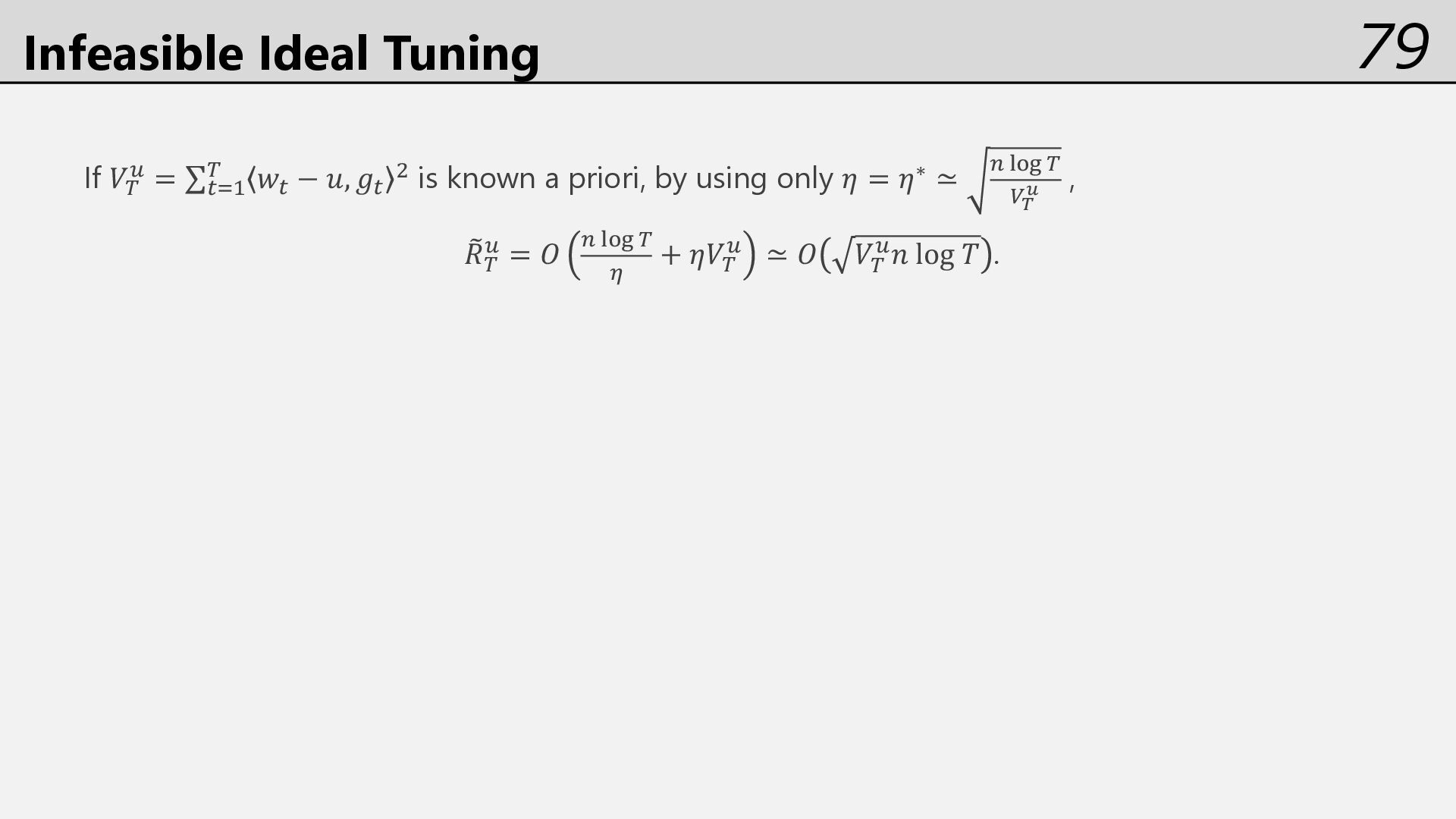
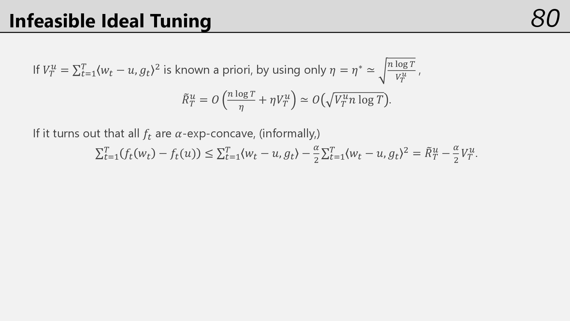
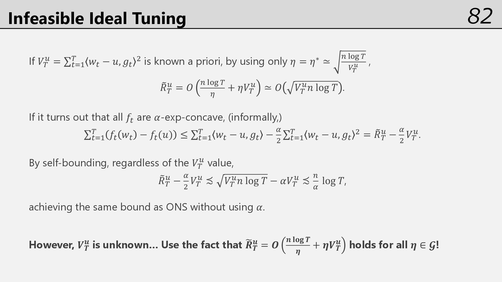
𝑤% − 𝑢, 𝑔% 5 is known a priori, by using only 𝜂 = 𝜂∗ ≃ " FGH ( I) 3 , O 𝑅( E = 𝑂 " FGH ( ; + 𝜂𝑉( E ≃ 𝑂 𝑉( E𝑛 log 𝑇 . If it turns out that all 𝑓% are 𝛼-exp-concave, (informally,) ∑%&' ( 𝑓% 𝑤% − 𝑓%(𝑢) ≤ ∑%&' ( 𝑤% − 𝑢, 𝑔% − 1 5 ∑%&' ( 𝑤% − 𝑢, 𝑔% 5 = O 𝑅( E − 1 5 𝑉( E.
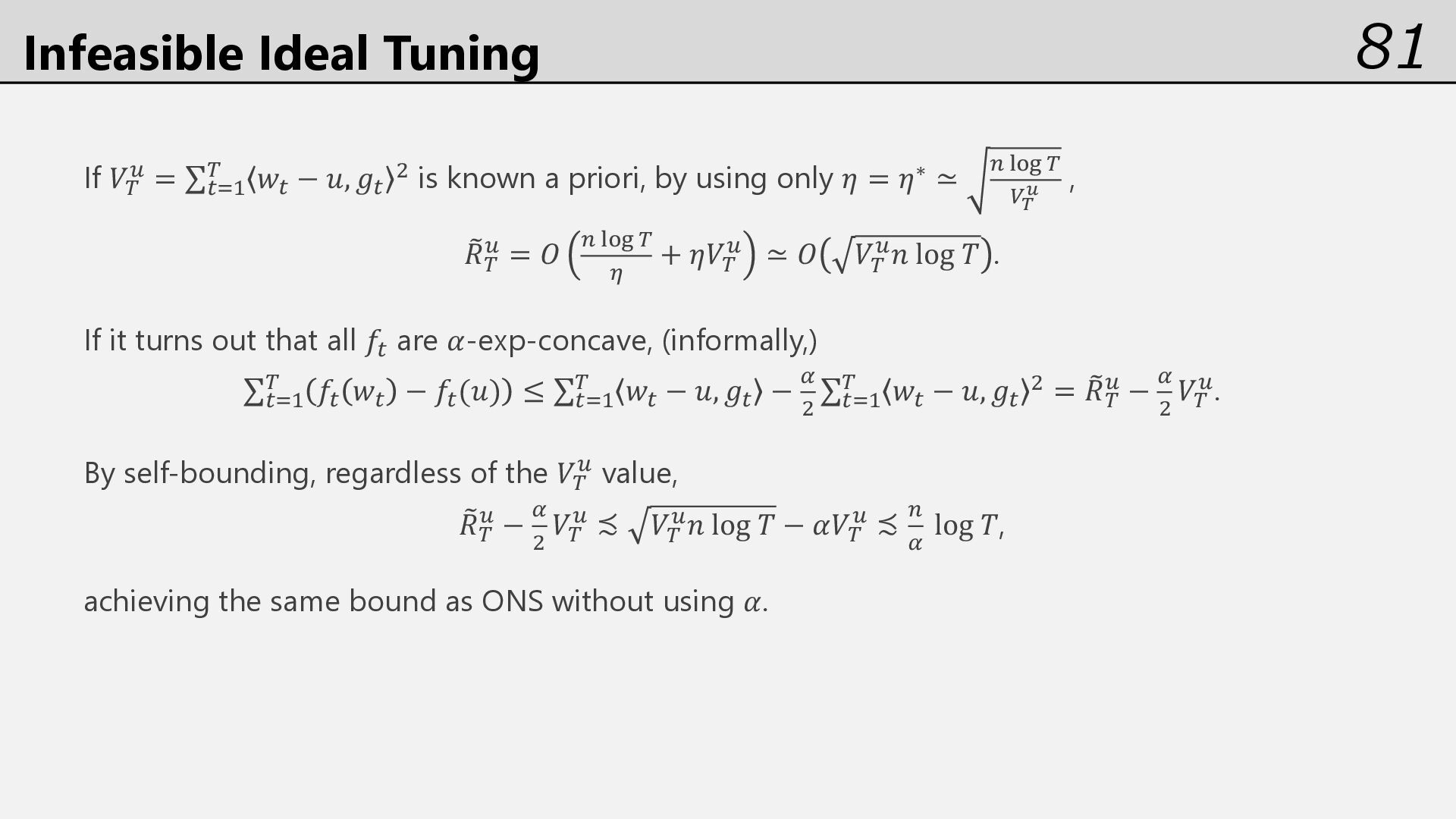
𝑤% − 𝑢, 𝑔% 5 is known a priori, by using only 𝜂 = 𝜂∗ ≃ " FGH ( I) 3 , O 𝑅( E = 𝑂 " FGH ( ; + 𝜂𝑉( E ≃ 𝑂 𝑉( E𝑛 log 𝑇 . If it turns out that all 𝑓% are 𝛼-exp-concave, (informally,) ∑%&' ( 𝑓% 𝑤% − 𝑓%(𝑢) ≤ ∑%&' ( 𝑤% − 𝑢, 𝑔% − 1 5 ∑%&' ( 𝑤% − 𝑢, 𝑔% 5 = O 𝑅( E − 1 5 𝑉( E. By self-bounding, regardless of the 𝑉( E value, O 𝑅( E − 1 5 𝑉( E ≾ 𝑉( E𝑛 log 𝑇 − 𝛼𝑉( E ≾ " 1 log 𝑇, achieving the same bound as ONS without using 𝛼.
𝑤% − 𝑢, 𝑔% 5 is known a priori, by using only 𝜂 = 𝜂∗ ≃ " FGH ( I) 3 , O 𝑅( E = 𝑂 " FGH ( ; + 𝜂𝑉( E ≃ 𝑂 𝑉( E𝑛 log 𝑇 . If it turns out that all 𝑓% are 𝛼-exp-concave, (informally,) ∑%&' ( 𝑓% 𝑤% − 𝑓%(𝑢) ≤ ∑%&' ( 𝑤% − 𝑢, 𝑔% − 1 5 ∑%&' ( 𝑤% − 𝑢, 𝑔% 5 = O 𝑅( E − 1 5 𝑉( E. By self-bounding, regardless of the 𝑉( E value, O 𝑅( E − 1 5 𝑉( E ≾ 𝑉( E𝑛 log 𝑇 − 𝛼𝑉( E ≾ " 1 log 𝑇, achieving the same bound as ONS without using 𝛼. However, 𝑽𝑻 𝒖 is unknown… Use the fact that „ 𝑹𝑻 𝒖 = 𝑶 𝒏 𝐥𝐨𝐠 𝑻 𝜼 + 𝜼𝑽𝑻 𝒖 holds for all 𝜼 ∈ 𝓖!
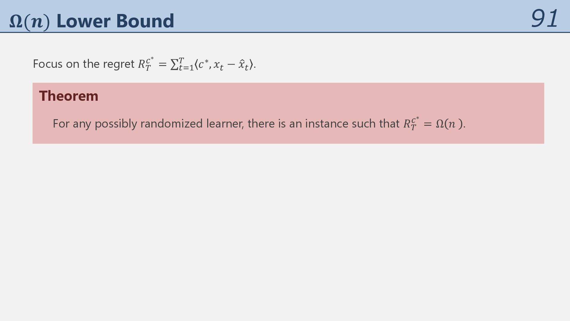
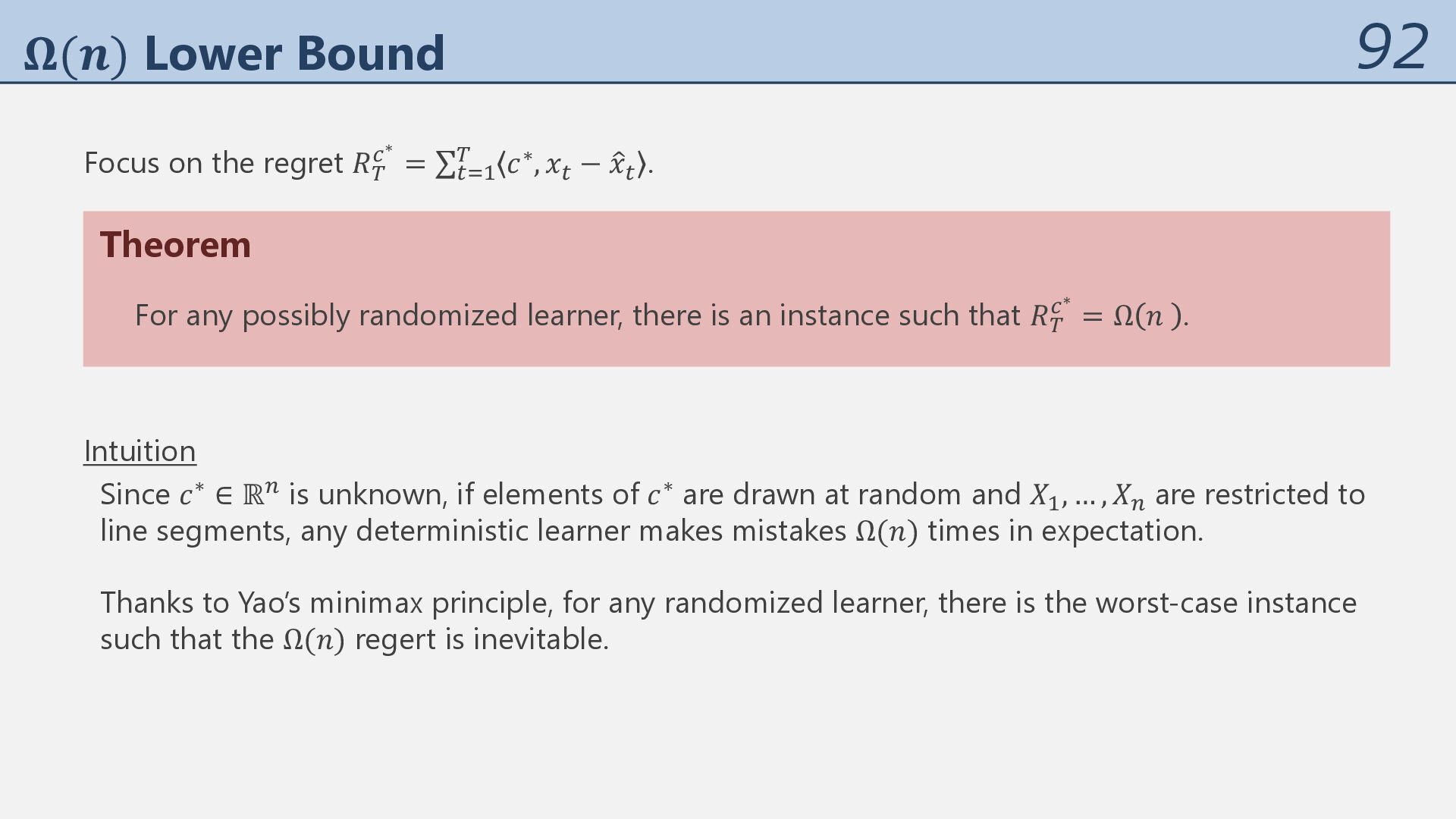
= ∑%&' ( 𝑐∗, 𝑥% − J 𝑥% . Theorem For any possibly randomized learner, there is an instance such that 𝑅( -∗ = Ω 𝑛 . Intuition Since 𝑐∗ ∈ ℝ" is unknown, if elements of 𝑐∗ are drawn at random and 𝑋', … , 𝑋" are restricted to line segments, any deterministic learner makes mistakes Ω(𝑛) times in expectation. Thanks to Yao’s minimax principle, for any randomized learner, there is the worst-case instance such that the Ω(𝑛) regert is inevitable.
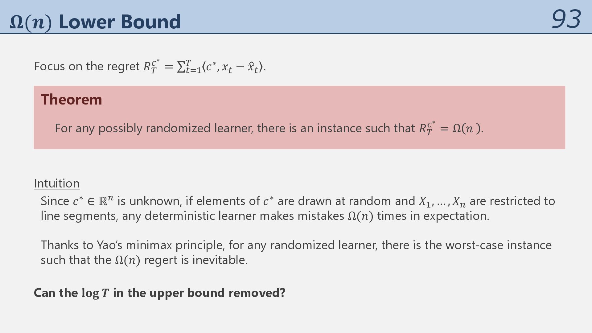
= ∑%&' ( 𝑐∗, 𝑥% − J 𝑥% . Theorem For any possibly randomized learner, there is an instance such that 𝑅( -∗ = Ω 𝑛 . Intuition Since 𝑐∗ ∈ ℝ" is unknown, if elements of 𝑐∗ are drawn at random and 𝑋', … , 𝑋" are restricted to line segments, any deterministic learner makes mistakes Ω(𝑛) times in expectation. Thanks to Yao’s minimax principle, for any randomized learner, there is the worst-case instance such that the Ω(𝑛) regert is inevitable. Can the 𝐥𝐨𝐠 𝑻 in the upper bound removed?
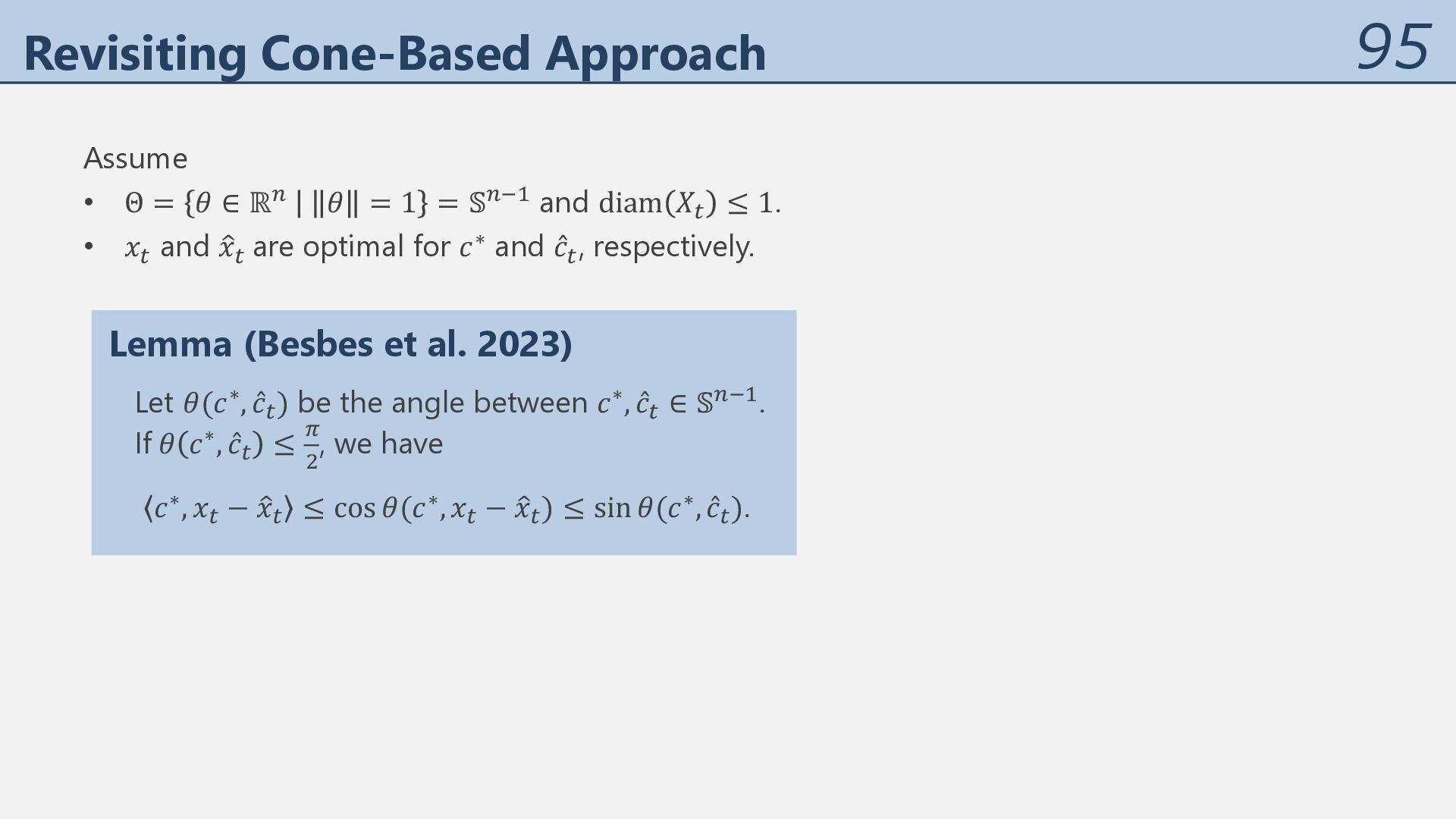
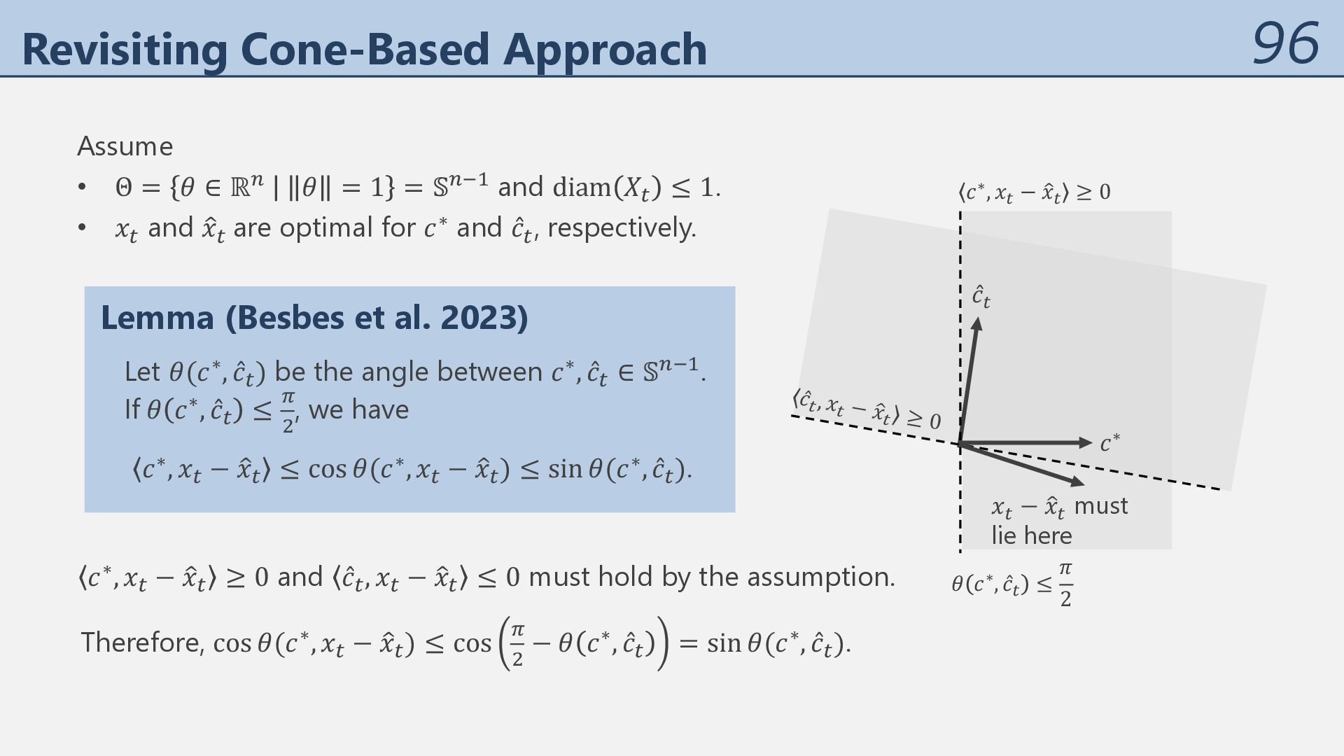
ℝ" 𝜃 = 1 = 𝕊"0' and diam 𝑋% ≤ 1. • 𝑥% and J 𝑥% are optimal for 𝑐∗ and ̂ 𝑐% , respectively. Lemma (Besbes et al. 2023) Let 𝜃(𝑐∗, ̂ 𝑐%) be the angle between 𝑐∗, ̂ 𝑐% ∈ 𝕊"0'. If 𝜃 𝑐∗, ̂ 𝑐% ≤ Q 5 , we have 𝑐∗, 𝑥% − J 𝑥% ≤ cos 𝜃(𝑐∗, 𝑥% − J 𝑥%) ≤ sin 𝜃(𝑐∗, ̂ 𝑐%).
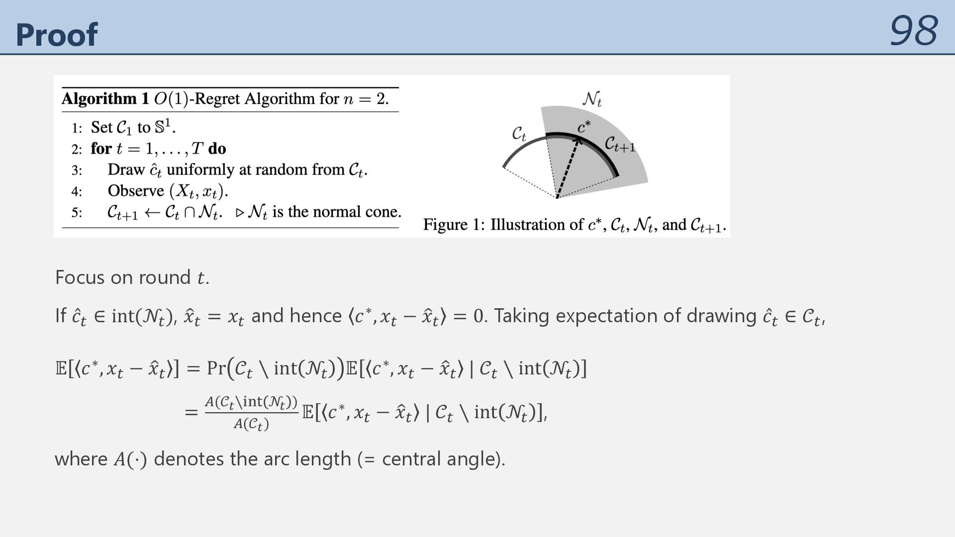
𝑇 (but extending to 𝑛 > 2 seems challenging, as discussed later). Theorem Algorithm 1 achieves 𝔼 𝑅( -∗ = 2𝜋. 𝒩% ≔ 𝑐 ∈ 𝕊' 𝑐, 𝑥% − 𝑥 ≥ 0 ∀𝑥 ∈ 𝑋% is the normal cone of 𝑋% at 𝑥% . 𝒞% is the region such that 𝑐∗ ∈ 𝒞% does not contradict “𝑥R ∈ arg max )∈+4 𝑐∗, 𝑥 for 𝑠 = 1, … , 𝑡 − 1.”