Optimal-Time Queries and Constructions of RLBWT in BWT-runs Bounded Space

This presentation slide is from a highlight session at CPM2024, which took place on June 27, 2024.
https://cpm2024.github.io/highlights.html

Transcript

1. Optimal-Time Queries and Constructions of RLBWT in BWT-runs Bounded Space Yasuo Tabei Collaboration with Takaaki Nishimoto and Shunsuke Kanda RIKEN-AIP (https://aip.riken.jp/) CPM2024-hightlight June 27, 2024
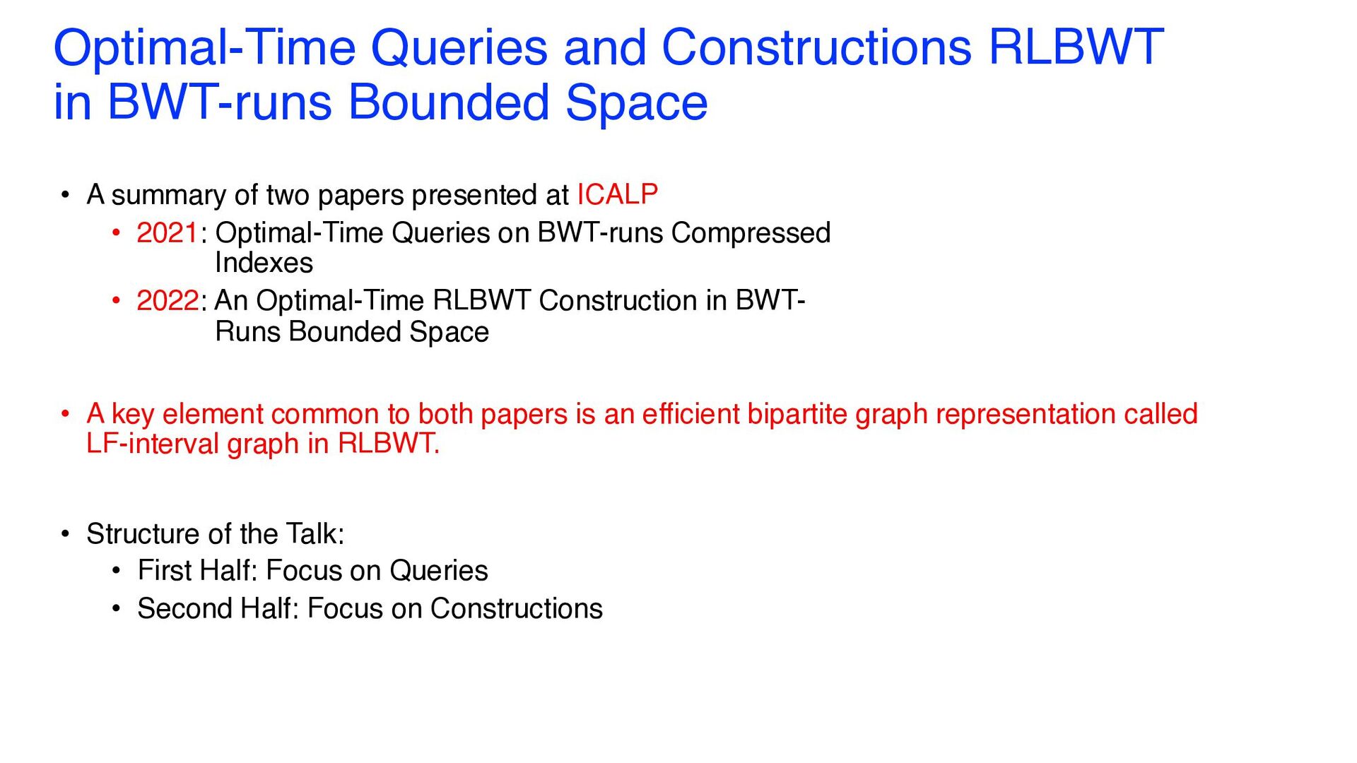
2. Optimal-Time Queries and Constructions RLBWT in BWT-runs Bounded Space • A summary of two papers presented at ICALP • 2021: Optimal-Time Queries on BWT-runs Compressed Indexes • 2022: An Optimal-Time RLBWT Construction in BWT- Runs Bounded Space • A key element common to both papers is an efficient bipartite graph representation called LF-interval graph in RLBWT. • Structure of the Talk: • First Half: Focus on Queries • Second Half: Focus on Constructions
3. Main Topic: Compressed Information Processing of Strings with Many Repetitions • Recently, strings characterized by many repetitions have become widespread in both research and industrial applications. Ex: Genome sequences, version-controlled documents, and more • Compressed information processing of these repetitive strings is a central research topic in string processing. • Several formats have been developed for this type of data, including grammars and LZ- type compressions. • We focus on RLBWT, a run-length compressed version of Burrows-Wheeler Transform (BWT) in this talk.
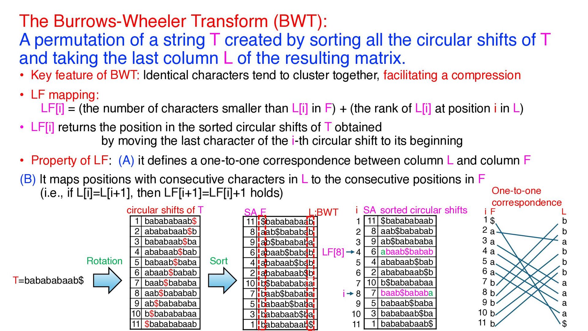
4. The Burrows-Wheeler Transform (BWT): A permutation of a string T created by sorting all the circular shifts of T and taking the last column L of the resulting matrix. • Key feature of BWT: Identical characters tend to cluster together, facilitating a compression • LF mapping: LF[i] = (the number of characters smaller than L[i] in F) + (the rank of L[i] at position i in L) • LF[i] returns the position in the sorted circular shifts of T obtained by moving the last character of the i-th circular shift to its beginning • Property of LF: (A) it defines a one-to-one correspondence between column L and column F (B) It maps positions with consecutive characters in L to the consecutive positions in F (i.e., if L[i]=L[i+1], then LF[i+1]=LF[i]+1 holds) 11 $babababaab 8 aab$bababab 9 ab$babababa 6 abaab$babab 4 ababaab$bab 2 abababaab$b 10 b$babababaa 7 baab$bababa 5 babaab$baba 3 bababaab$ba 1 babababaab$ 1 babababaab$ 2 abababaab$b 3 bababaab$ba 4 ababaab$bab 5 babaab$baba 6 abaab$babab 7 baab$bababa 8 aab$bababab 9 ab$babababa 10 b$babababaa 11 $babababaab T=babababaab$ L:BWT _ Sort circular shifts of T Rotation F SA $ a a a a a b b b b b b b a b b b a a a a $ F L 1 2 3 4 5 6 7 8 9 10 11 i sorted circular shifts 1 2 3 4 5 6 7 8 9 10 11 i SA 11 $babababaab 8 aab$bababab 9 ab$babababa 6 abaab$babab 4 ababaab$bab 2 abababaab$b 10 b$babababaa 7 baab$bababa 5 babaab$baba 3 bababaab$ba 1 babababaab$ i LF[8] One-to-one correspondence
5. Backward Search Using LF-mapping : Find the SA-interval [s,t] of pattern P on L ① Initialize [s,t] = [1,|L|] and h = |P| ② Find the first and last occurrence positions [k,ℓ] of character P[h] in the interval [s,t] on L - Rank and select on L are used for computing [k,ℓ] ③ Compute s’=LF[k] and t’=LF[ℓ] using LF-mapping • Every element j ∈ [s’,t’] satisfies the condition that suffix P[h..|P|] is a prefix of suffix T[SA[ j ]..|T|] ④ Update s=s’, t=t’, h=h–1, and go to step① if s ≦ t or h>0 hold • Complexity: O(|P| log σ) time and O(|T| log σ) bits of space (σ : alphabet size) sorted circular shifts 1 2 3 4 5 6 7 8 9 10 11 F L 1 2 3 4 5 6 7 8 9 10 11 i s’ t’ $ a a a a a b b b b b b b a b b b a a a a $ Input P=aba h=1 [s,t]=[8,11] k ℓ s t Output [s’,t’]=[4,6] i SA 11 $babababaab 8 aab$bababab 9 ab$babababa 6 abaab$babab 4 ababaab$bab 2 abababaab$b 10 b$babababaa 7 baab$bababa 5 babaab$baba 3 bababaab$ba 1 babababaab$ ① ② ③ P[1]=a
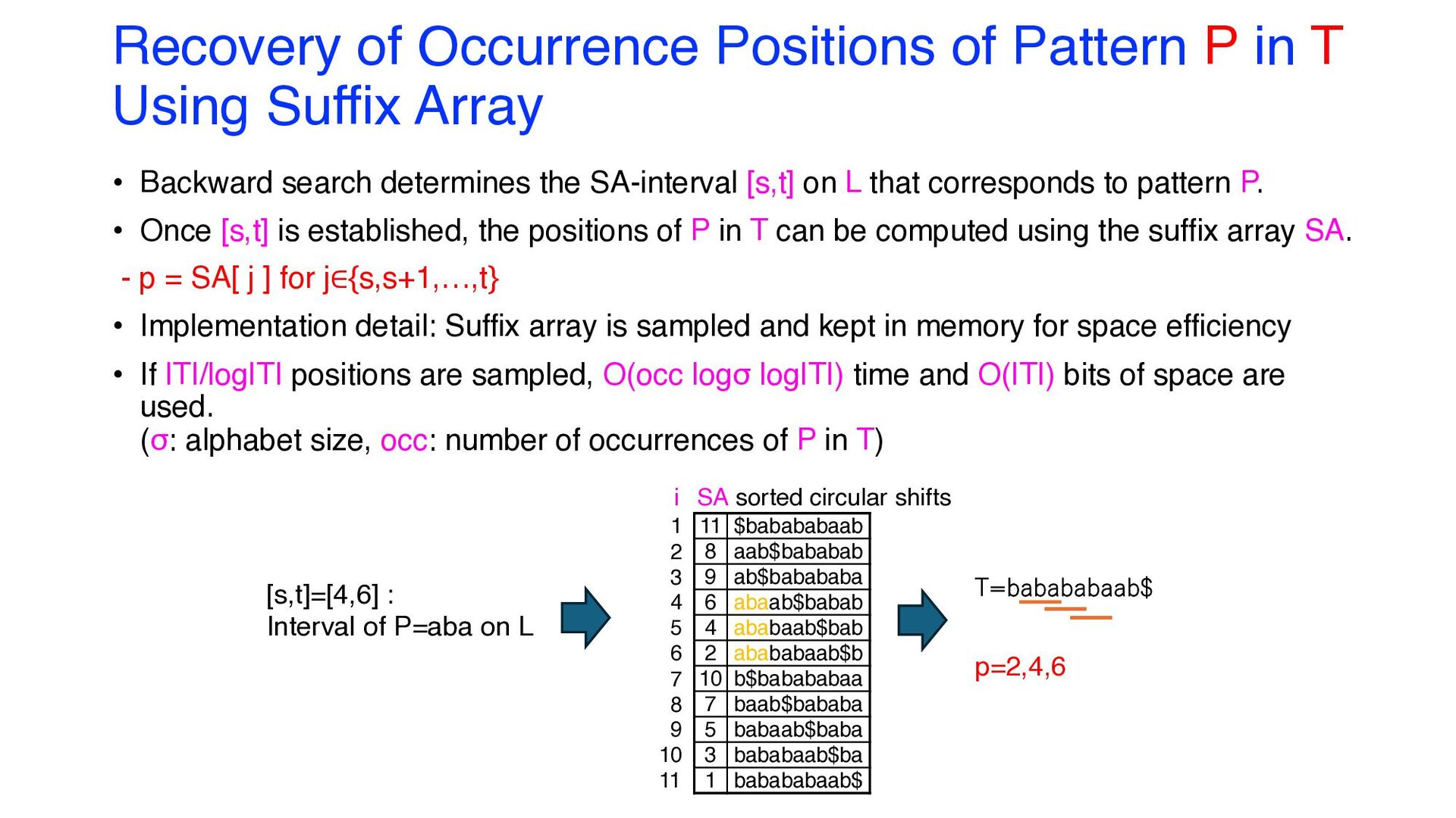
6. Recovery of Occurrence Positions of Pattern P in T Using Suffix Array • Backward search determines the SA-interval [s,t] on L that corresponds to pattern P. • Once [s,t] is established, the positions of P in T can be computed using the suffix array SA. - p = SA[ j ] for j∈{s,s+1,…,t} • Implementation detail: Suffix array is sampled and kept in memory for space efficiency • If |T|/log|T| positions are sampled, O(occ logσ log|T|) time and O(|T|) bits of space are used. (σ: alphabet size, occ: number of occurrences of P in T) [s,t]=[4,6] : Interval of P=aba on L p=2,4,6 T=babababaab$ 11 $babababaab 8 aab$bababab 9 ab$babababa 6 abaab$babab 4 ababaab$bab 2 abababaab$b 10 b$babababaa 7 baab$bababa 5 babaab$baba 3 bababaab$ba 1 babababaab$ 1 2 3 4 5 6 7 8 9 10 11 i SA sorted circular shifts
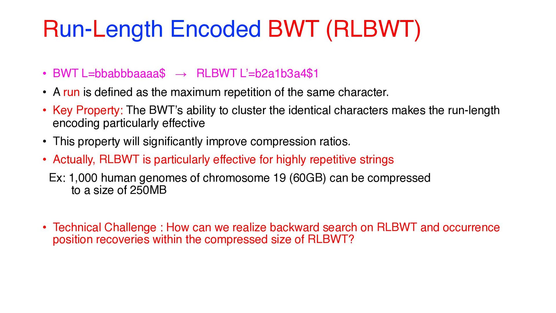
7. Run-Length Encoded BWT (RLBWT) • BWT L=bbabbbaaaa$ → RLBWT L’=b2a1b3a4$1 • A run is defined as the maximum repetition of the same character. • Key Property: The BWT’s ability to cluster the identical characters makes the run-length encoding particularly effective • This property will significantly improve compression ratios. • Actually, RLBWT is particularly effective for highly repetitive strings Ex: 1,000 human genomes of chromosome 19 (60GB) can be compressed to a size of 250MB • Technical Challenge : How can we realize backward search on RLBWT and occurrence position recoveries within the compressed size of RLBWT?
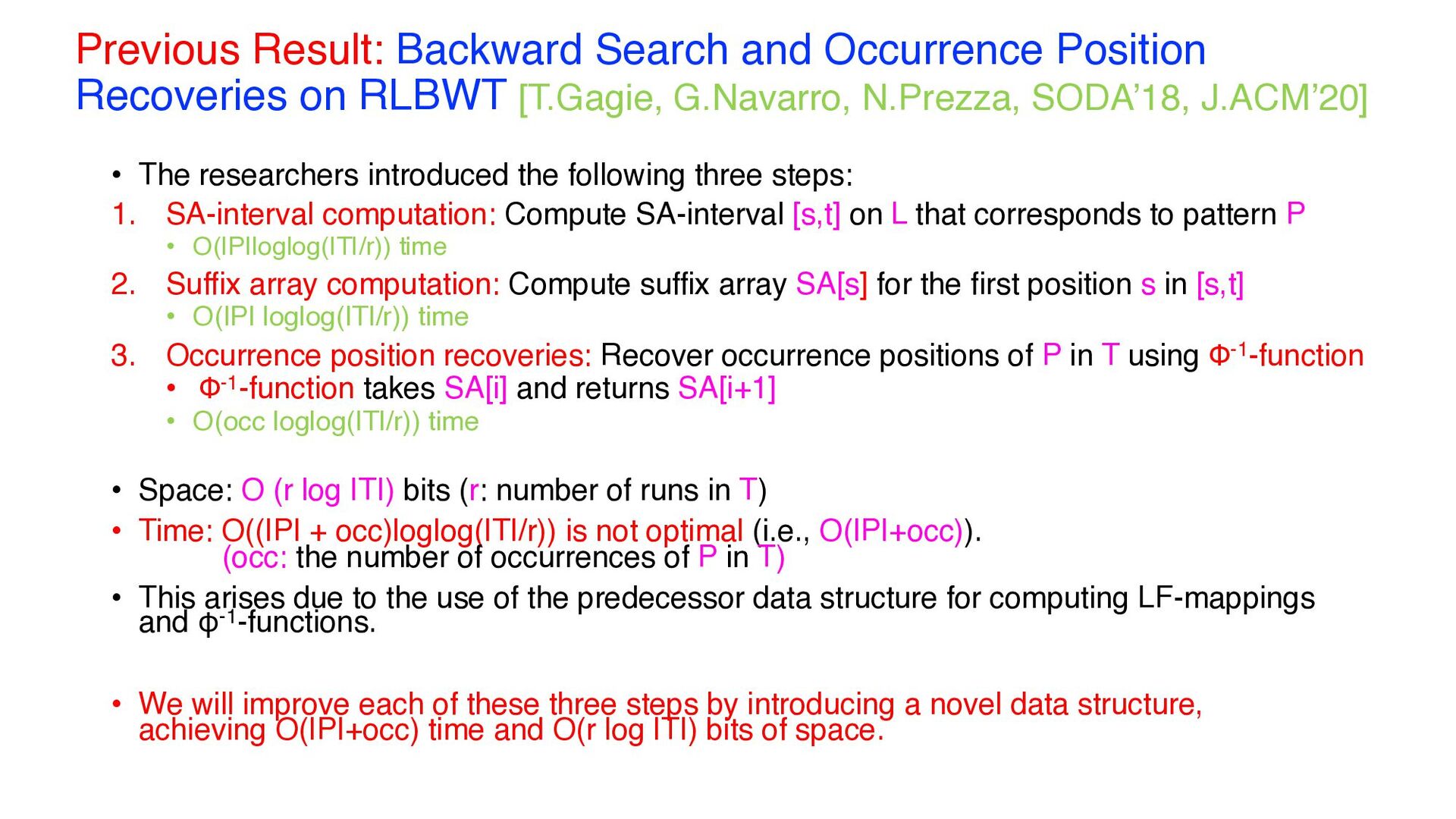
8. Previous Result: Backward Search and Occurrence Position Recoveries on RLBWT [T.Gagie, G.Navarro, N.Prezza, SODA’18, J.ACM’20] • The researchers introduced the following three steps: 1. SA-interval computation: Compute SA-interval [s,t] on L that corresponds to pattern P • O(|P|loglog(|T|/r)) time 2. Suffix array computation: Compute suffix array SA[s] for the first position s in [s,t] • O(|P| loglog(|T|/r)) time 3. Occurrence position recoveries: Recover occurrence positions of P in T using Φ-1-function • Φ-1-function takes SA[i] and returns SA[i+1] • O(occ loglog(|T|/r)) time • Space: O (r log |T|) bits (r: number of runs in T) • Time: O((|P| + occ)loglog(|T|/r)) is not optimal (i.e., O(|P|+occ)). (occ: the number of occurrences of P in T) • This arises due to the use of the predecessor data structure for computing LF-mappings and φ-1-functions. • We will improve each of these three steps by introducing a novel data structure, achieving O(|P|+occ) time and O(r log |T|) bits of space.
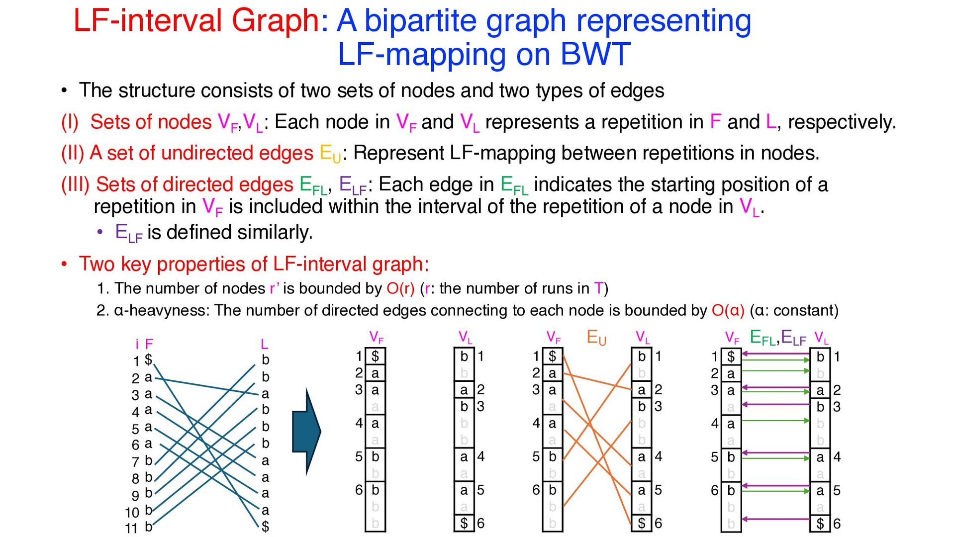
9. LF-interval Graph: A bipartite graph representing LF-mapping on BWT • The structure consists of two sets of nodes and two types of edges (I) Sets of nodes VF ,VL : Each node in VF and VL represents a repetition in F and L, respectively. (II) A set of undirected edges EU : Represent LF-mapping between repetitions in nodes. (III) Sets of directed edges EFL , ELF : Each edge in EFL indicates the starting position of a repetition in VF is included within the interval of the repetition of a node in VL . • ELF is defined similarly. • Two key properties of LF-interval graph: 1. The number of nodes r’ is bounded by O(r) (r: the number of runs in T) 2. α-heavyness: The number of directed edges connecting to each node is bounded by O(α) (α: constant) $ a a a a a b b b b b b b a b b b a a a a $ F L 1 2 3 4 5 6 7 8 9 10 11 i VF VL EU EFL ,ELF $ a a a a a b b b b b 1 2 3 4 5 6 b b a b b b a a a a $ 1 2 3 4 5 6 VF VL $ a a a a a b b b b b 1 2 3 4 5 6 b b a b b b a a a a $ 1 2 3 4 5 6 VF VL $ a a a a a b b b b b 1 2 3 4 5 6 b b a b b b a a a a $ 1 2 3 4 5 6
10. Backward Search on LF-interval Graphs : Find SA-interval [s,t] of pattern P on L • LF-interval graph is traversed as performed during the backward search in the BWT • k: the first position on L such that L[k]=c holds for (i) a given character c in P and (ii) a given SA-interval. • u: the first node including position k on L in the repetition of u • There are two important issues to be solved in backward search on LF-interval graph: Q1: Which element d in the repetition of node u' on VF corresponds to the s'-th element on F, where s' = LF[k]? Q2: Which node on VL contains the s’-th element in L in the repetition? .. a a a a a a .. b b b b .. b b a b b .. a a a a a u’ VF VL EU u k s’=LF[k] d .. a a a a a a .. b b b b .. b b a b b .. a a a a a u’ VF VL s’=LF[k] EFL x s’ ELF Figure for Q1 Figure for Q2
11. Backward Search on LF-interval Graphs : Find SA-interval [s,t] of pattern P on L Q1: Which element d in the repetition of node u' on VF corresponds to the s'-th element on F, where s' = LF[k]? A1: Use the following property of LF-mapping: Consecutive characters on u are mapped to consecutive ones on u’ • Thus, d is preserved in the two repetitions of nodes u and u’ connected by an undirected edge • The d-th element in the repetition of u’ on VF are computed from the same d-th element in the repetition of u on VL .. a a a a a a .. b b b b .. b b a b b .. a a a a a u’ VF VL EU k s’=LF[k] d d u Figure for Q1
12. Backward Search on LF-interval Graphs : Find SA-interval [s,t] of pattern P on L Q2: Which node on VL contains the s’-th element in L in the repetition? A2: Use this fact: Such node must connect to u’ by a directed edge in EFL or ELF . • Let x be the node connected to u’ by a directed edge in EFL • A linear search starting from x on VL can find a node including the s’-th element • Use array AL : which includes starting positions of the repetition of each node on VL • Computation time: O(α) • This efficiency is due to the number of nodes connected to u’ by directed edges being O(α) .. a a a a a a .. b b b b .. b b a b b .. a a a a a u’ VF VL s’=LF[k] EFL x s’ ELF Figure for Q2
13. Compute suffix array SA[s] for the first position s in SA-interval [s,t] • Idea : Leverage the property of LF-mapping: SA[LF[i]]=SA[i]-1 • Thus, we can compute SA[s’] for the first position s’ of the next SA-interval [s’,t’] from SA[s] for the first position s of the current SA-interval [s,t]. • Compute SA[s’] as follows: Case (i): If c=L[k] corresponds to the first character of the repetition of u, SA[s’] = SASAMP_F [u] - 1 Case (ii): Otherwise, SA[s’] = SA[s] - 1 • Array SASAMP_F : sampled SA according to the starting position of the repetition of each node in VL • The computation is valid because case (i) must hold at the first iteration in the backward search. .. a a a a a a .. b b b b .. b b a b b .. a a a a a u’ VF VL s’=LF[k] EFL x s’ ELF EU k u s t
14. Computing Φ-1-function : Given SA[i], it returns SA[i+1] • Idea : (i) Build a partite graph that represents the relationship between input SA[i] and output SA[i+1] and (ii) compute Φ-1-function on the graph • Set of nodes SAsamp : Includes sampled SA according to the ending position of the repetition for each node on VL • Set of nodes Φ-1(SAsamp ) : Includes SA[i+1] if SA[i] is included in SAsamp • Undirected edges E’U : An edge connecting SAsamp [ i ] to Φ-1(SAsamp )[ j ] indicates Φ-1(SAsamp )[ j ] = SA[i+1] holds • Directed edges ERL : Each position i in Φ-1(SAsamp ) is included within the interval of a node in SAsamp. 11 8 9 6 4 2 10 7 5 3 1 SA VL b b a b b b a a a a $ 1 2 3 4 5 6 SAsamp 11 8 9 6 4 2 10 7 5 3 1 11 9 6 10 5 1 Φ-1(SAsamp ) SAsamp 1 2 3 4 5 6 7 8 9 10 11 1 2 3 4 5 6 7 8 9 10 11 Φ-1(SAsamp ) SAsamp 1 2 3 4 5 6 7 8 9 10 11 1 2 3 4 5 6 7 8 9 10 11 Φ-1(SAsamp ) SAsamp 1 2 3 4 5 6 7 8 9 10 11 1 2 3 4 5 6 7 8 9 10 11 Φ-1(SAsamp ) (i)Sampling (ii)Sort (iii)Build edges E’U ERL
15. Computing Φ-1-function : Given SA[i], it returns SA[i+1] (Cont.) • For a given position i in SA-interval [s,t], let u be the node on SASAMP that contains SA[i] within the interval. • Let v be the node connected to node u by an undirected edge in E’U • Φ-1(SA[i]) is computed by leveraging the following property: Each node in SASAMP represents the consecutive SA’s values; The consecutive SA’s values in each node are also mapped to Φ-1(SAsamp ) as the same consecutive values. • Can compute Φ-1(SA[i]) as follows: Φ-1(SA[i])=Φ-1(SAsamp )[v]+(SA[i] − SAsamp [u]) • Detail: The next u corresponding to the computed Φ-1(SA[i]) is obtained using a linear search on SAsamp , starting from u’ connected to v by the directed edge in ERL (O(α) time) SAsamp 1 2 3 4 5 6 7 8 9 10 11 1 2 3 4 5 6 7 8 9 10 11 Φ-1(SAsamp ) SAsamp 1 2 3 4 5 6 7 8 9 10 11 1 2 3 4 5 6 7 8 9 10 11 Φ-1(SAsamp ) E’U ERL SA[i] u v Φ-1(SA[i]) Example for SA[i]=6: u=3, v=1 Φ-1(6)=Φ-1(SAsamp )[1]+(6-SAsamp [3]) =1+(6-3) =4 =d d d
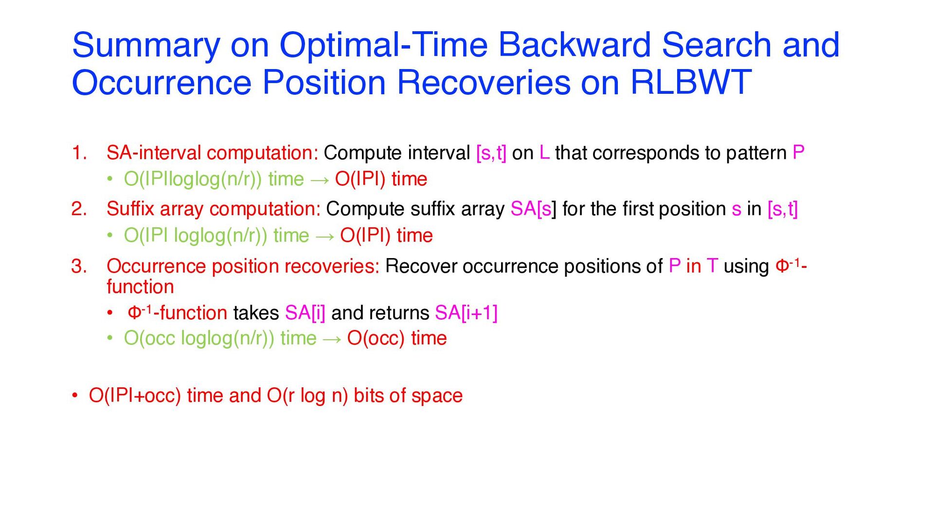
16. Summary on Optimal-Time Backward Search and Occurrence Position Recoveries on RLBWT 1. SA-interval computation: Compute interval [s,t] on L that corresponds to pattern P • O(|P|loglog(n/r)) time → O(|P|) time 2. Suffix array computation: Compute suffix array SA[s] for the first position s in [s,t] • O(|P| loglog(n/r)) time → O(|P|) time 3. Occurrence position recoveries: Recover occurrence positions of P in T using Φ-1- function • Φ-1-function takes SA[i] and returns SA[i+1] • O(occ loglog(n/r)) time → O(occ) time • O(|P|+occ) time and O(r log n) bits of space
17. •Optima-Time Construction of RLBWT
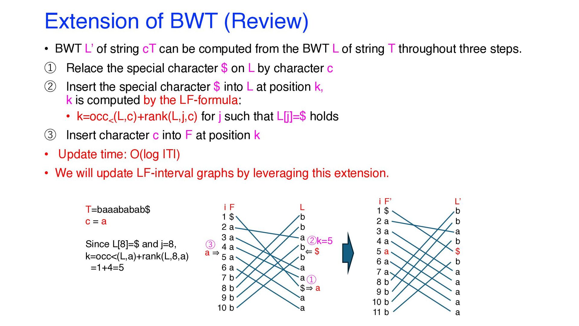
18. Extension of BWT (Review) • BWT L’ of string cT can be computed from the BWT L of string T throughout three steps. ① Relace the special character $ on L by character c ② Insert the special character $ into L at position k, k is computed by the LF-formula: • k=occ< (L,c)+rank(L,j,c) for j such that L[j]=$ holds ③ Insert character c into F at position k • Update time: O(log |T|) • We will update LF-interval graphs by leveraging this extension. $ a a a a a a b b b b b b a b $ b a a a a a F’ L’ 1 2 3 4 5 6 7 8 9 10 11 i $ a a a a a b b b b b b a b b a a $ a a F L 1 2 3 4 5 6 7 8 9 10 i ⇒ a ⇐ $ T=baaababab$ c = a Since L[8]=$ and j=8, k=occ<(L,a)+rank(L,8,a) =1+4=5 ① ②k=5 ③ a ⇒
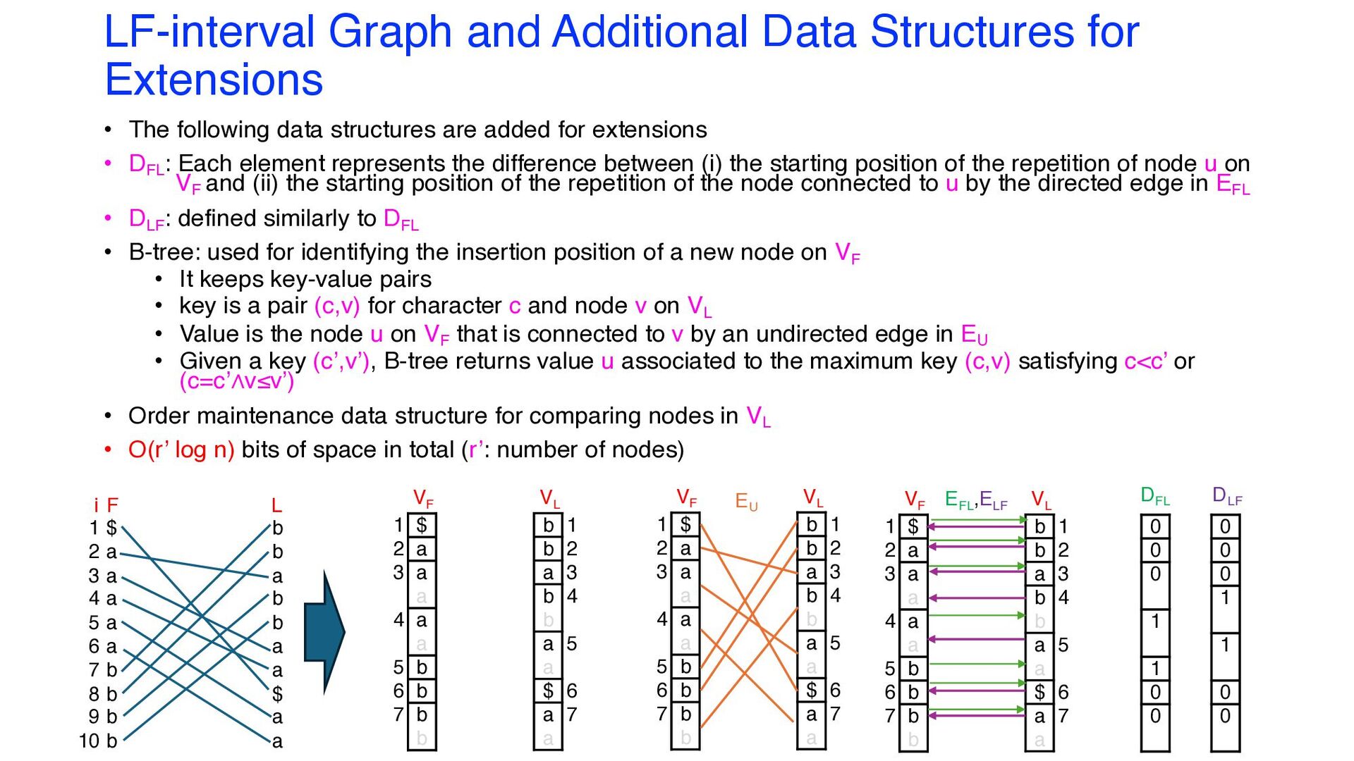
19. LF-interval Graph and Additional Data Structures for Extensions • The following data structures are added for extensions • DFL : Each element represents the difference between (i) the starting position of the repetition of node u on VF and (ii) the starting position of the repetition of the node connected to u by the directed edge in EFL • DLF : defined similarly to DFL • B-tree: used for identifying the insertion position of a new node on VF • It keeps key-value pairs • key is a pair (c,v) for character c and node v on VL • Value is the node u on VF that is connected to v by an undirected edge in EU • Given a key (c’,v’), B-tree returns value u associated to the maximum key (c,v) satisfying c<c’ or (c=c’∧v≤v’) • Order maintenance data structure for comparing nodes in VL • O(r’ log n) bits of space in total (r’: number of nodes) VF VL EU $ a a a a a b b b b 1 2 3 4 5 6 7 b b a b b a a $ a a 1 2 3 4 5 6 7 $ a a a a a b b b b b b a b b a a $ a a F L 1 2 3 4 5 6 7 8 9 10 i VF VL $ a a a a a b b b b 1 2 3 4 5 6 7 b b a b b a a $ a a 1 2 3 4 5 6 7 VF VL $ a a a a a b b b b 1 2 3 4 5 6 7 b b a b b a a $ a a 1 2 3 4 5 6 7 EFL ,ELF 0 0 0 1 1 0 0 DFL 0 0 0 1 1 0 0 DLF
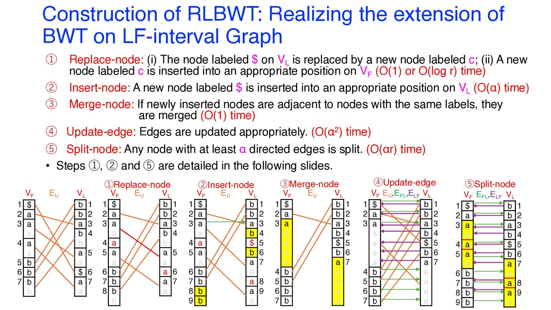
20. Construction of RLBWT: Realizing the extension of BWT on LF-interval Graph ① Replace-node: (i) The node labeled $ on VL is replaced by a new node labeled c; (ii) A new node labeled c is inserted into an appropriate position on VF (O(1) or O(log r) time) ② Insert-node: A new node labeled $ is inserted into an appropriate position on VL (O(α) time) ③ Merge-node: If newly inserted nodes are adjacent to nodes with the same labels, they are merged (O(1) time) ④ Update-edge: Edges are updated appropriately. (O(α2) time) ⑤ Split-node: Any node with at least α directed edges is split. (O(αr) time) • Steps ①, ② and ⑤ are detailed in the following slides. EU VF VL $ a a a a a b b b b 1 2 3 4 5 6 7 b b a b b a a $ a a 1 2 3 4 5 6 7 ①Replace-node VF VL $ a a a a a a b b b b 1 2 3 4 5 6 7 8 b b a b b a a a a a 1 2 3 4 5 6 7 EU VF VL $ a a a a a a b b b b 1 2 3 4 5 6 7 8 9 b b a b $ b a a a a a 1 2 3 4 5 6 7 8 9 EU ②Insert-node VF VL $ a a a a a a b b b b 1 2 3 4 5 6 7 b b a b $ b a a a a a 1 2 3 4 5 6 7 EU ③Merge-node VF VL $ a a a a a a b b b b 1 2 3 4 5 6 7 b b a b $ b a a a a a 1 2 3 4 5 6 7 EU ,EFL ,ELF ④Update-edge VF VL $ a a a a a a b b b b 1 2 3 4 5 6 7 8 9 b b a b $ b a a a a a 1 2 3 4 5 6 7 8 9 EFL ,ELF ⑤Split-node
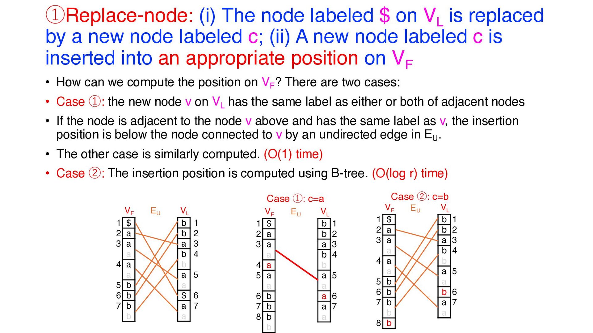
21. ①Replace-node: (i) The node labeled $ on VL is replaced by a new node labeled c; (ii) A new node labeled c is inserted into an appropriate position on VF • How can we compute the position on VF ? There are two cases: • Case ①: the new node v on VL has the same label as either or both of adjacent nodes • If the node is adjacent to the node v above and has the same label as v, the insertion position is below the node connected to v by an undirected edge in EU . • The other case is similarly computed. (O(1) time) • Case ②: The insertion position is computed using B-tree. (O(log r) time) EU VF VL $ a a a a a b b b b 1 2 3 4 5 6 7 b b a b b a a $ a a 1 2 3 4 5 6 7 Case ①: c=a VF VL $ a a a a a a b b b b 1 2 3 4 5 6 7 8 b b a b b a a a a a 1 2 3 4 5 6 7 EU VF VL $ a a a a a b b b b b 1 2 3 4 5 6 7 8 b b a b b a a b a a 1 2 3 4 5 6 7 EU Case ②: c=b
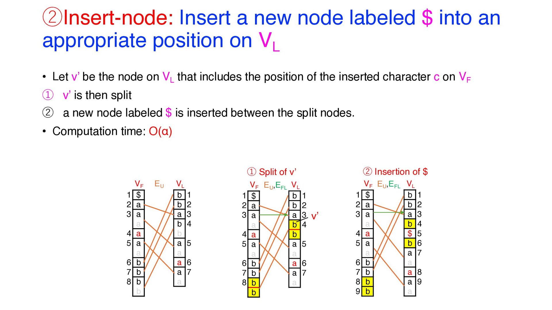
22. ②Insert-node: Insert a new node labeled $ into an appropriate position on VL • Let v’ be the node on VL that includes the position of the inserted character c on VF ① v’ is then split ② a new node labeled $ is inserted between the split nodes. • Computation time: O(α) VF VL $ a a a a a a b b b b 1 2 3 4 5 6 7 8 b b a b b a a a a a 1 2 3 4 5 6 7 EU VF VL $ a a a a a a b b b b 1 2 3 4 5 6 7 8 9 b b a b $ b a a a a a 1 2 3 4 5 6 7 8 9 VF VL $ a a a a a a b b b b 1 2 3 4 5 6 7 8 b b a b b a a a a a 1 2 3 4 5 6 7 EU ,EFL EU ,EFL ① Split of v’ ② Insertion of $ v’
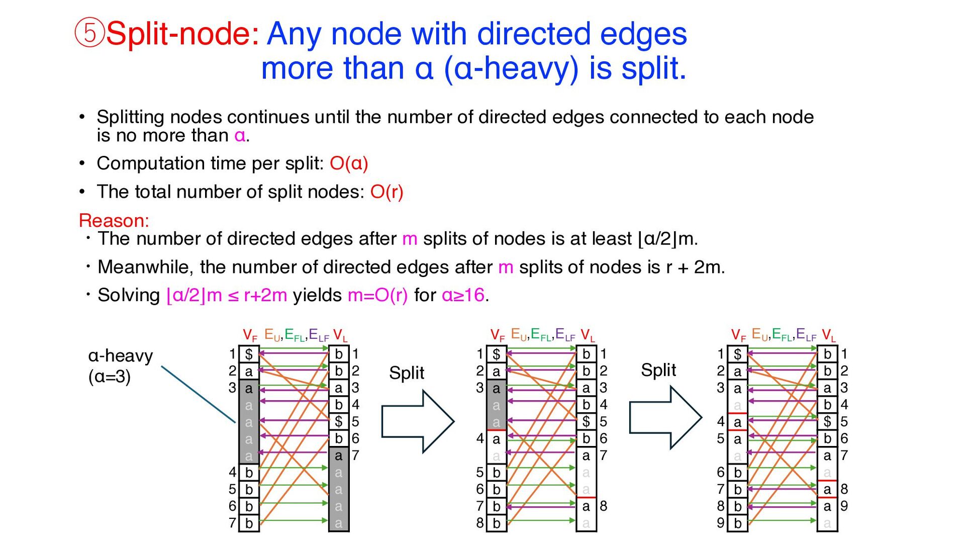
23. ⑤Split-node: Any node with directed edges more than α (α-heavy) is split. • Splitting nodes continues until the number of directed edges connected to each node is no more than α. • Computation time per split: O(α) • The total number of split nodes: O(r) Reason: ・The number of directed edges after m splits of nodes is at least ⌊α/2⌋m. ・Meanwhile, the number of directed edges after m splits of nodes is r + 2m. ・Solving ⌊α/2⌋m ≤ r+2m yields m=O(r) for α≥16. VF VL $ a a a a a a b b b b 1 2 3 4 5 6 7 b b a b $ b a a a a a 1 2 3 4 5 6 7 VF VL $ a a a a a a b b b b 1 2 3 4 5 6 7 8 b b a b $ b a a a a a 1 2 3 4 5 6 7 8 EU ,EFL ,ELF EU ,EFL ,ELF VF VL $ a a a a a a b b b b 1 2 3 4 5 6 7 8 9 b b a b $ b a a a a a 1 2 3 4 5 6 7 8 9 EU ,EFL ,ELF α-heavy (α=3) Split Split
24. Experimental Results on A Large Dataset Dataset String σ |T| [103] r [103] boost 96 1,073,769 65 enwiki 207 37,849,201 70,190 chr19.1000 5 59,125,169 45,143 • R-comp (this study) is compared to 1. PP: A.Policriti and N.Prezza, 2018 2. Faster-PP: T. Ohno et al., 2018. >24hours 10GB
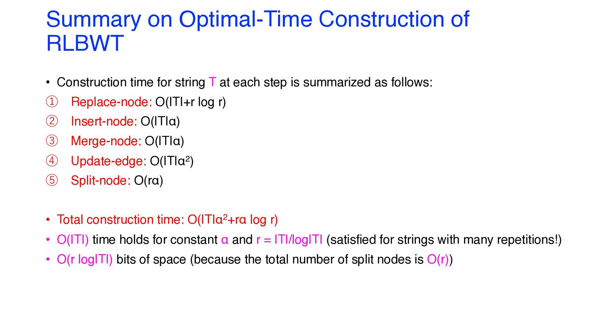
25. Summary on Optimal-Time Construction of RLBWT • Construction time for string T at each step is summarized as follows: ① Replace-node: O(|T|+r log r) ② Insert-node: O(|T|α) ③ Merge-node: O(|T|α) ④ Update-edge: O(|T|α2) ⑤ Split-node: O(rα) • Total construction time: O(|T|α2+rα log r) • O(|T|) time holds for constant α and r = |T|/log|T| (satisfied for strings with many repetitions!) • O(r log|T|) bits of space (because the total number of split nodes is O(r))
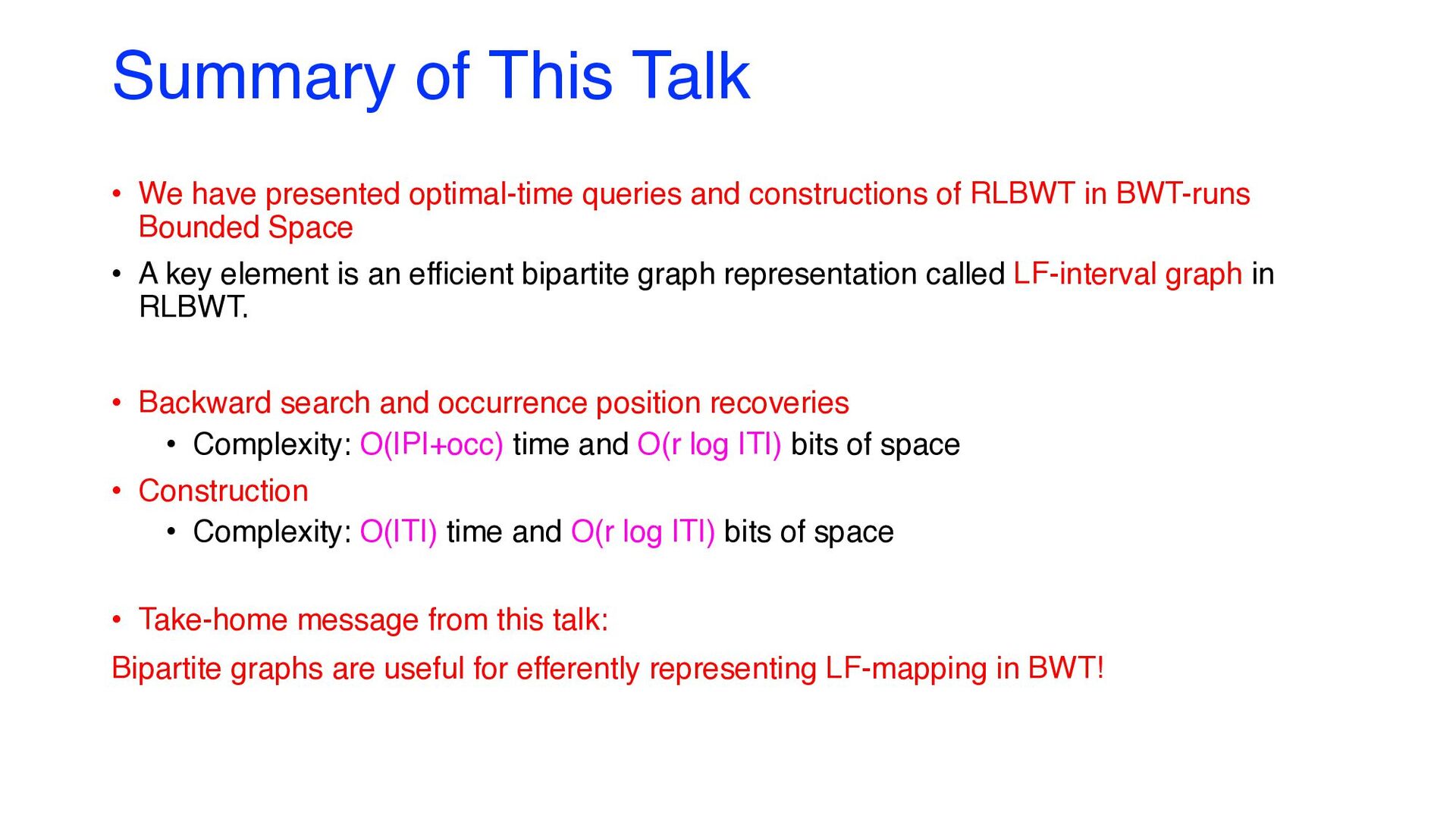
26. Summary of This Talk • We have presented optimal-time queries and constructions of RLBWT in BWT-runs Bounded Space • A key element is an efficient bipartite graph representation called LF-interval graph in RLBWT. • Backward search and occurrence position recoveries • Complexity: O(|P|+occ) time and O(r log |T|) bits of space • Construction • Complexity: O(|T|) time and O(r log |T|) bits of space • Take-home message from this talk: Bipartite graphs are useful for efferently representing LF-mapping in BWT!