Quorum sensing without counting, a discounting approach, or: Nobody goes there anymore, it’s too crowded

Quorum sensing is ubiquitous in nature, but the underlying mechanisms that individuals use to sense quorums are not well understood beyond bacterial quorum sensing. Encounter rate appears to be an important cue of quorum attainment in ants, but how ants synthesize their individual-level experiences to determine whether they have reached a critical encounter rate is still unknown. Computer scientists have suggested quorum-sensing strategies that are implemented on an individual agents with some way to count discrete encounters with other individuals. Instead, motivated by observations of honeybees and classic research on temporal discounting in psychology, we propose a quorum sensing algorithm based on the likelihood that an ant will re-encounter a nest entrance within a short time period of the last encounter with another ant. Simulations of the resulting mechanism show both outcome and response-time characteristics that are qualitatively similar to ants, and the implementation does not require maintaining a count of previous encounters with other agents.

Transcript

1. Quorum sensing without counting, a discounting approach “Nobody goes there anymore, it’s too crowded” …or… Collaborators: Jake Hanson, Dr. Gabriele Valentini, Dr. Sara Imari Walker, Dr. Stephen C. Pratt Dr. Theodore (Ted) P. Pavlic Assistant Professor School of Computing, Informatics, and Decision Systems Engineering School of Sustainability School of Life Sciences Arizona State University (Tempe, AZ, USA)
2. (via Matthew Ryan and Laura Washburn) 2 Bacterial Quorum Sensing
3. Injection Site Target Site Bio−Nano Robot Concentration Gradient Swarm Intelligence for Cooperation of Bio-Nano Robots using Quorum Sensing Sreedevi Chandrasekaran and Dean F. Hougen ract— Bio-nano robots are nano-scaled robots made from cal components like proteins and DNA structures. Their caled size, ready availability (in nature), and high effi- make them perfect tools for diagnosis and therapeutic ents in nano-medicine. Due to their nano-scaled size, elligence of each individual nano robot is small when red to that of the collection of nano robots acting together omplish the given task. This group intelligence, called intelligence, helps the nano robots do their task more ely, more quickly, and with fewer other resources. The nation to accomplish the given task can be achieved by nano robots through quorum sensing. Quorum sensing ability of nano robots to communicate and coordinate or via signaling molecules. The whole scenario of com- ation and coordination can be done using these nano- robots and the results are studied using simulation at a vel of abstraction. I. INTRODUCTION obot is an autonomous physical device where sensing ctions are coupled by intelligent decisions [1]. A no robot is a nano-scaled biologically-based robot. robot systems and find that the performance is of the changes greatly by varying the quorum threshold val The research presented here will help future bi robot designers and developers to decide among v design strategies before they start constructing these of bio-nano robots for real world applications. A. Methods for Nano Intelligence Unlike traditional robots, bio-nano robots require niques such as swarm intelligence and quorum sensi efficient performance because of their space limitatio 1) Swarm Intelligence: Every nano-robot perform same set of tasks to accomplish a goal, for example, a tumor site in an affected individual. Instead of doi difficult task on it’s own, nano-robots can communica coordinate as a group to accomplish the desired goa collective behavior, that emerges from a group of indiv insignificant agents, is called swarm intelligence [7]. intelligence happens widely in nature, for examp (Chandrasekaran and Hougen, 2006, ASM-IEEE Conference on Bio-, Micro- and Nanosystems) 3
4. Crevice-dwelling, house-hunting Temnothorax ants (© James Waters, Takao Sasaki) 4
5. “Tandem running” behavior (via Stephen C. Pratt) Propensity to do a tandem run increases with nest-site quality 5
6. “Transport” behavior (via Stephen C. Pratt) Transport triggered by candidate site reaching quorum 6
7. (Pratt, 2005, Behav. Ecol.) Decision Accuracy 7
8. “Counting and Calculating” Swarm Intell (2010) 4: 199–220 Fig. 2 This figure illustrates the principle behind analog consensus estimation (ACE). Each robot its own quorum and kin index, both of which decay exponentially at the same rate. A robot incre kin index every time that a teammate is encountered. The quorum index is incremented only by de robots, after they have encountered a teammate that agrees that the current task is complete. The ra peak equilibria of a robot’s quorum and kin indices approximates the apparent consensus Assume that each robot in a well-stirred dec-MRS will encounter one of its tea every T0 seconds on average. Each robot therefore will increment its kin index mately every T0 seconds. Each deliberating robot will tend to encounter an agreein mate every T0/Ca seconds on average, and so they will increment their quorum in this rate. It was shown in Parker (2009) that the peak equilibria of the quorum and kin (qequ and kequ , respectively) are given by qequ = ∆ 1 − e −T0 τCa ≈ ∆ τCa T0 , kequ = ∆ 1 − e −T0 τ ≈ ∆ τ T0 . The ratio of a deliberating robot’s two indices’ peak values at equilibria, qequ kequ , mates the apparent consensus, Ca . In Fig. 2, the quorum index is incremented half as the kin index; its peak value at equilibrium is approximately 50% of that of th The accuracies of the rightmost terms of (2) increase with τ, making the delibera bots’ estimates of Ca more precise as the indices are made to decay more slowly re Musco, Su, and Lynch (2017, PNAS) [BDA 2016] Parker and Zhang (2010, Swarm Int.) Parker and Zhang (2009, IEEE/ASME Trans. Mechatronics) Parker and Zhang (IROS 2004) “Counting and Thresholding” upper threshold lower threshold positive decision negative decision internal state indicator (a) Peysakhov and Regli (SIS 2005) Approaches from Engineering and Computer Science 8
9. to slowly mixing graphs, showing that strong local mixing is suffi- cient in many applications. The key to the local mixing property of the grid is an upper bound on the probability that two random walks starting from the same position recollide (or that a single random walk equal- izes) after a certain number of steps (Lemma 3). We show that recollision probability bounds imply collision moment bounds on general graphs, and apply this technique to extend our results to d-dimensional grids, regular expanders, and hypercubes. We dis- cuss applications of our bounds to the task of estimating the size of a social network using random walks (12), obtaining improve- ments over prior work for networks with relatively slow global mixing times but strong local mixing. We also discuss connections to density estimation by robot swarms and random walk-based sensor network sampling (13, 14). Theoretical Model for Density Estimation We consider a set of agents populating a 2D torus with A nodes (dimensions p A ⇥ p A). At each time step, each agent has an associated ordered pair position, which gives its coordinates on the torus. We assume that A is large—larger than the area agents traverse over the runtimes of our algorithms. We believe the torus model successfully captures the dynamics of density estima- tion on a surface, while avoiding complicating factors of bound- ary behavior on a finite grid. Initially, each agent is placed independently at a uniform ran- dom node in the torus. Computation proceeds in discrete, syn- chronous rounds. Each agent updates its position with a step cho- sen uniformly at random from {(0, 1), (0, 1), (1, 0), ( 1, 0)} in each round. Of course, in reality, ants do not move via pure ran- dom walk; observed encounter rates seem to actually be lower than predicted by a pure random walk model (6, 15). How- ever, we feel that our model sufficiently captures the highly ran- Fig. 1. A basic illustration of our computational model. Each agent (ant) may move to a random adjacent position on the 2D torus in each round (illustrated by the red arrows). A collision occurs when two or more agents are located at the same position. The agents detect collisions through the count(position) function, which returns the number of other agents at their current position. In this illustration, position is given as the (x, y) position, with the bottom left corner corresponding to (1, 1). However, the precise convention used is unimportant. Musco et al. PNAS | October 3, 2017 | vol. 114 | no. 40 | 10535 for simplicity. Removing our assumption of uniformly distributed agents and understanding local density estimation are important directions for future work. Random Walk-Based Density Estimation on the 2D Torus As discussed, the challenge in analyzing random walk-based den- sity estimation on the torus arises from correlations between col- lisions of nearby agents. If we do not restrict agents to random walking, and instead allow each agent to take an arbitrary step in each round, they can avoid collision correlations by splitting into “stationary” and “mobile” groups and counting collisions only between members of different groups. This allows them to essentially simulate independent sampling of grid locations to estimate density. This method is simple to analyze (SI Appendix, section S1), but it is not “natural” in a biological sense or useful for the applications we present. Further, independent sampling is unnecessary! Algorithm 1 describes a simple random walk-based approach that gives a nearly matching bound. Our main theoretical result follows; its proof appears at the end of this section, after a number of preliminary lemmas. Throughout our analysis, we take the viewpoint of a single agent executing Algorithm 1. never meet via random walking. Howeve change the expectation of ˜ d computed ab not affect any of our following proofs. With Lemma 2 in place, it remains to sho rate is close to its expectation with high p vides a good estimate of density. To do the strength of correlations between collis in successive rounds, which can decrease encounter rate-based estimate. A Recollision Probability Bound. The key correlations is bounding the probability of two agents in round r +m, assuming a colli we do in this section. Let cj = P t r=1 cj (r) be the total num agent j. Due to the initial uniform distribu cj are all independent and identically distr Each cj is the sum of highly correlate due to the slow mixing of the grid, if t round r, they are much more likely to rounds. However, by bounding this recol are able to give strong moment bounds f each cj . We bound not only its variance bu This allows us to show that the aver falls close to its expectation d with hig Theorem 1. Lemma 3 (Recollision Probability Bound). C and a2 randomly walking on a 2D torus of d If a1 and a2 collide in round r , for any m a1 and a2 collide again in round r +m is ⇥ ( • Nearby agents collide repeatedly • Cannot recognize duplicate collisions • Yet counting algorithm will converge to actual density Number of rounds t chosen by ant/evolution. 9
10. to slowly mixing graphs, showing that strong local mixing is suffi- cient in many applications. The key to the local mixing property of the grid is an upper bound on the probability that two random walks starting from the same position recollide (or that a single random walk equal- izes) after a certain number of steps (Lemma 3). We show that recollision probability bounds imply collision moment bounds on general graphs, and apply this technique to extend our results to d-dimensional grids, regular expanders, and hypercubes. We dis- cuss applications of our bounds to the task of estimating the size of a social network using random walks (12), obtaining improve- ments over prior work for networks with relatively slow global mixing times but strong local mixing. We also discuss connections to density estimation by robot swarms and random walk-based sensor network sampling (13, 14). Theoretical Model for Density Estimation We consider a set of agents populating a 2D torus with A nodes (dimensions p A ⇥ p A). At each time step, each agent has an associated ordered pair position, which gives its coordinates on the torus. We assume that A is large—larger than the area agents traverse over the runtimes of our algorithms. We believe the torus model successfully captures the dynamics of density estima- tion on a surface, while avoiding complicating factors of bound- ary behavior on a finite grid. Initially, each agent is placed independently at a uniform ran- dom node in the torus. Computation proceeds in discrete, syn- chronous rounds. Each agent updates its position with a step cho- sen uniformly at random from {(0, 1), (0, 1), (1, 0), ( 1, 0)} in each round. Of course, in reality, ants do not move via pure ran- dom walk; observed encounter rates seem to actually be lower than predicted by a pure random walk model (6, 15). How- ever, we feel that our model sufficiently captures the highly ran- Fig. 1. A basic illustration of our computational model. Each agent (ant) may move to a random adjacent position on the 2D torus in each round (illustrated by the red arrows). A collision occurs when two or more agents are located at the same position. The agents detect collisions through the count(position) function, which returns the number of other agents at their current position. In this illustration, position is given as the (x, y) position, with the bottom left corner corresponding to (1, 1). However, the precise convention used is unimportant. Musco et al. PNAS | October 3, 2017 | vol. 114 | no. 40 | 10535 Is counting and calculating the right computational model for ant quorum sensing? Is there a simpler way for robotic quorum sensing and other spatial applications? 11
11. (Pavlic and Pratt, in prep) Decision Latency 12 Number of rounds t chosen adaptively? During counting process? Like an adaptive step size in a numerical solver?
12. (Pavlic and Pratt, in prep) Psychological Review 1999, Vol. 106, No. 2, 261-300 Copyright 1999 by the American Psychological Association, Inc. 0033-295X/99/S3.00 Connectionist and Diffusion Models of Reaction Time Roger Ratcliff Northwestern University Trisha Van Zandt Johns Hopkins University Gail McKoon Northwestern University Two connectionist frameworks, GRAIN (J. L. McClelland, 1993) and brain-state-in-a-box (J. A. Anderson, 1991), and R. Ratcliff s (1978) diffusion model were evaluated using data from a signal detection task. Dependent variables included response probabilities, reaction times for correct and error responses, and shapes of reaction-time distributions. The diffusion model accounted for all aspects of the data, including error reaction times that had previously been a problem for all response-time models. The connectionist models accounted for many aspects of the data adequately, but each failed to a greater or lesser degree in important ways except for one model that was similar to the diffusion model. The findings advance the development of the diffusion model and show that the long tradition of reaction- time research and theory is a fertile domain for development and testing of connectionist assumptions about how decisions are generated over time. Research aimed at investigating how information is processed over time has had a long and influential history in psychology. In 1938 in his general textbook, Woodworm discussed simple and choice reaction time, the behaviors and shapes of reaction-time distributions, individual differences in reaction time, and the ef- fects on reaction time of experimental variables such as stimulus intensity. Several of these topics are raised again in this article. In the 1960s, when the cognitive revolution gave rise to modern cognitive psychology, reaction time entered the spotlight as a Connectionist models are a relatively new class of models and a surge in development and testing of them has taken place in the last 10 years. These models offer the promise of explanations of how cognitive tasks are learned. For most of the models, learning is the result of many individual trials with stimuli, each trial with feedback about whether the model's response was correct. The processes by which the response to a stimulus is chosen are usually assumed to be parallel, interactive, nonlinear, and continuous. These processing characteristics are theoretical choices that have Could a ants be using the same mechanisms for quorum detection as humans? used in fitting were chosen to represent widely spaced parts of the latency-response probability function (Figure 3). For example, for Subject 1, the values of response probability chosen were 0.965, 0.463, and 0.143. Each of these three values actually corresponds to two sets of reaction-time data, the number for which the probability of a high response equaled the chosen value and the number for which the probability of a low response equaled the chosen value. The fitting program adjusted the three values of v plus the three other parameters (a, 17, and Tfr ) to minimize a sum of squares using a standard function minimization routine. The data for the different subjects were fit individually, so the three values of v plus the other three parameters all were free to vary across subjects. The parameter estimates are shown in Table 1. Respond High Respond Low Parameters of the Diffusion Model: a = Boundary position z = starting point = a/2 v = mean drift rate, one for each condition s = standard deviation in drift within a trial Ter = encoding and response time i\ = standard deviation in mean drift rate from trial to trial (drift is N(v,n)) ex-Gaussians served as a meeting point between and the theoretical predictions from the model sents the position of the leading edge of the represents the extent of the tail of the distribu squares function was the sum of squared differ theoretically derived and empirically derived Gaussian summary parameters plus the sum of s in the theoretical and empirical values of respon weighted by standard errors). The fitting rout sums of squares as a function of the diffusion (see the Appendix for a full presentation). (The third parameter, cr, which roughly specifies the edge of the distribution, but it is not needed be model produces a rise in the reaction-time distri to the rise observed in the experimental data.) A shown in the figures are direct fits of the model recent work, we have moved to fitting the reac tions directly using quantiles of the distribution are not different in the two procedures. As pointed out, the three values of v for merely representative of all of the 96 experime served the purpose of summarizing the range o the other three parameter values, a, T), and Te subject. To sweep out all the conditions, v m some very low value to some very high value. I of the conditions were accommodated by v ra +.4, where a drift rate of -.4 corresponde 1 Note that setting up a successful run of the fi requires one or more runs much of the way through equaled the chosen value. The fitting program adjusted the three values of v plus the three other parameters (a, 17, and Tfr ) to minimize a sum of squares using a standard function minimization routine. The data for the different subjects were fit individually, so the three values of v plus the other three parameters all were free to vary across subjects. The parameter estimates are shown in Table 1. Respond High Respond Low Parameters of the Diffusion Model: a = Boundary position z = starting point = a/2 v = mean drift rate, one for each condition s = standard deviation in drift within a trial Ter = encoding and response time i\ = standard deviation in mean drift rate from trial to trial (drift is N(v,n)) sz =standard deviation in starting point (starting point is N(z,sz )) Figure 7. The diffusion model and parameters of the model. 13
13. Psychological Review 1999, Vol. 106, No. 2, 261-300 Copyright 1999 by the American Psychological Association, Inc. 0033-295X/99/S3.00 Connectionist and Diffusion Models of Reaction Time Roger Ratcliff Northwestern University Trisha Van Zandt Johns Hopkins University Gail McKoon Northwestern University Two connectionist frameworks, GRAIN (J. L. McClelland, 1993) and brain-state-in-a-box (J. A. Anderson, 1991), and R. Ratcliff s (1978) diffusion model were evaluated using data from a signal detection task. Dependent variables included response probabilities, reaction times for correct and error responses, and shapes of reaction-time distributions. The diffusion model accounted for all aspects of the data, including error reaction times that had previously been a problem for all response-time models. The connectionist models accounted for many aspects of the data adequately, but each failed to a greater or lesser degree in important ways except for one model that was similar to the diffusion model. The findings advance the development of the diffusion model and show that the long tradition of reaction- time research and theory is a fertile domain for development and testing of connectionist assumptions about how decisions are generated over time. Research aimed at investigating how information is processed over time has had a long and influential history in psychology. In 1938 in his general textbook, Woodworm discussed simple and choice reaction time, the behaviors and shapes of reaction-time distributions, individual differences in reaction time, and the ef- fects on reaction time of experimental variables such as stimulus intensity. Several of these topics are raised again in this article. In the 1960s, when the cognitive revolution gave rise to modern cognitive psychology, reaction time entered the spotlight as a Connectionist models are a relatively new class of models and a surge in development and testing of them has taken place in the last 10 years. These models offer the promise of explanations of how cognitive tasks are learned. For most of the models, learning is the result of many individual trials with stimuli, each trial with feedback about whether the model's response was correct. The processes by which the response to a stimulus is chosen are usually assumed to be parallel, interactive, nonlinear, and continuous. These processing characteristics are theoretical choices that have 14 “Counting and Thresholding” upper threshold lower threshold positive decision negative decision internal state indicator (a) Peysakhov and Regli (SIS 2005)
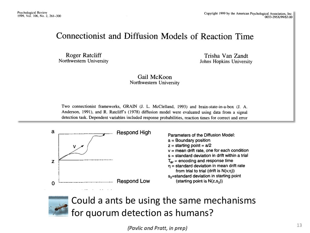
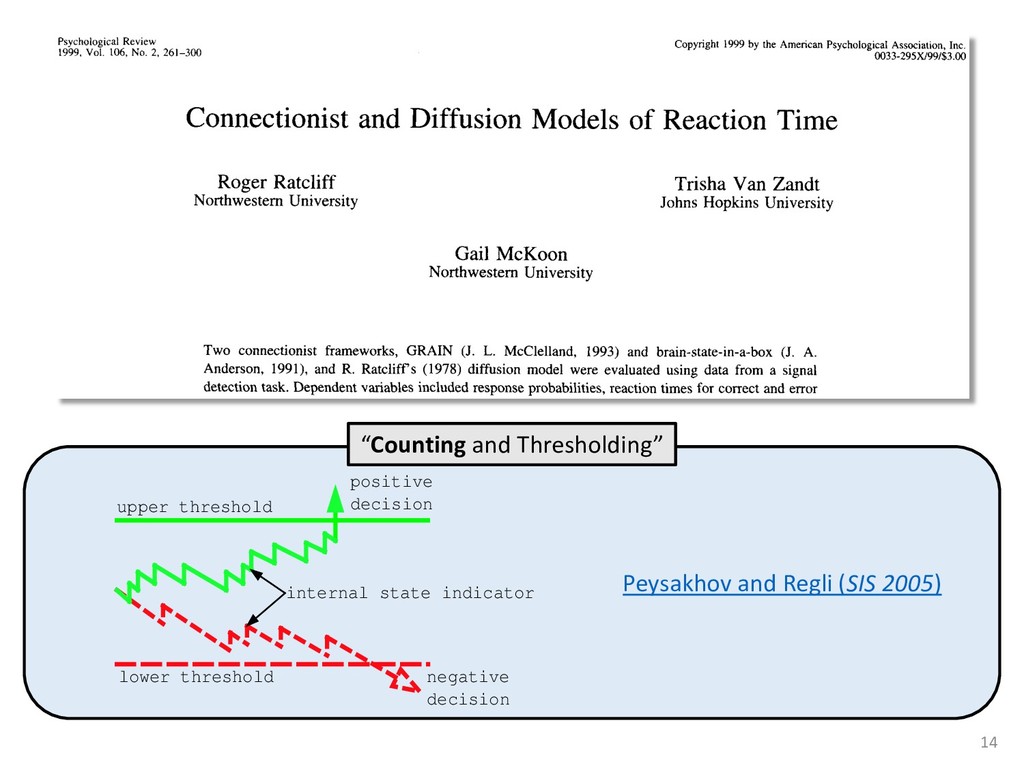
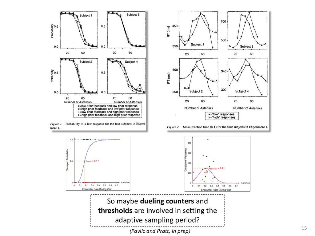
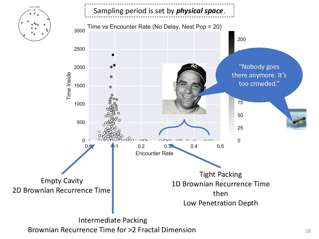
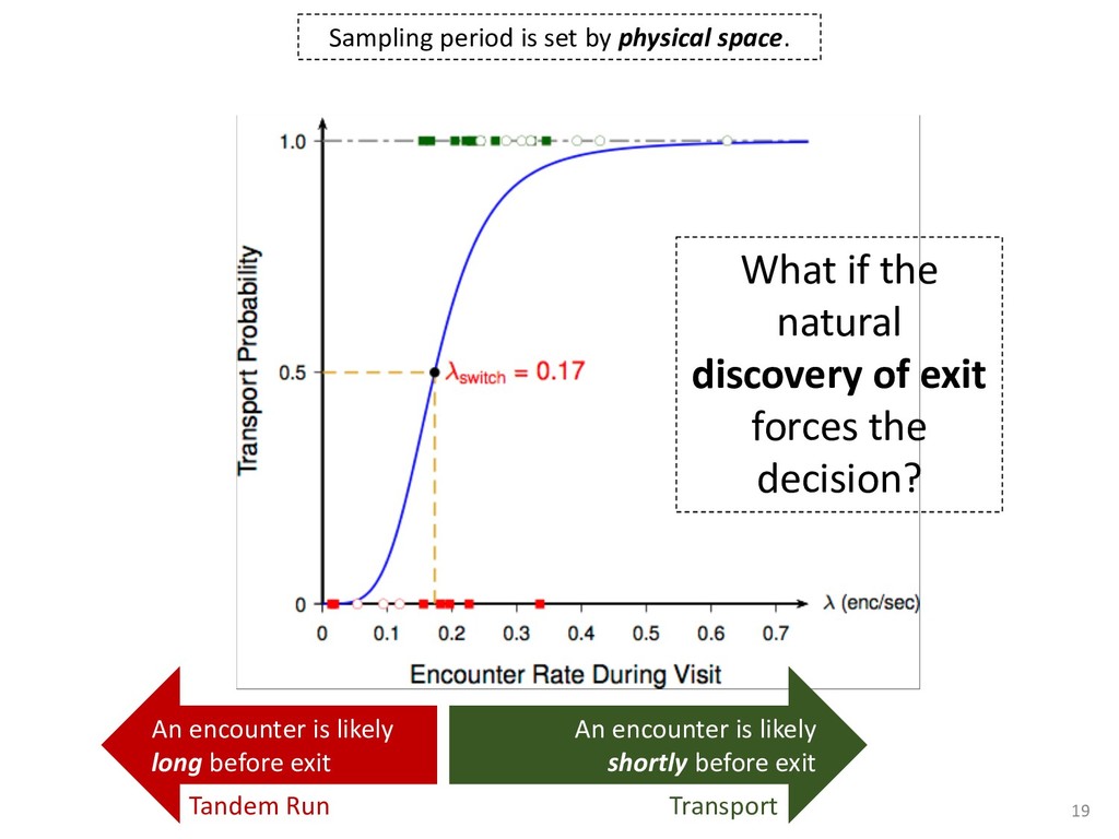
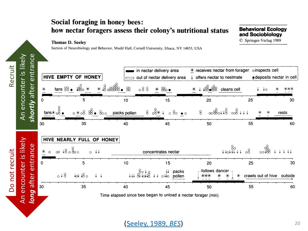
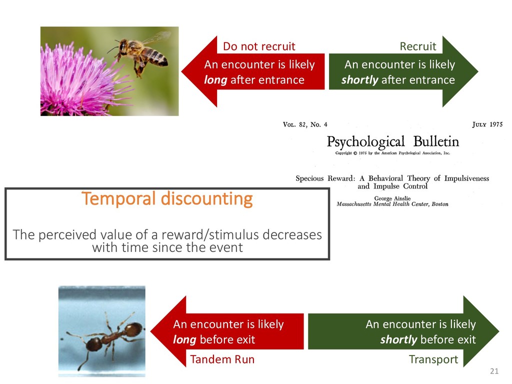
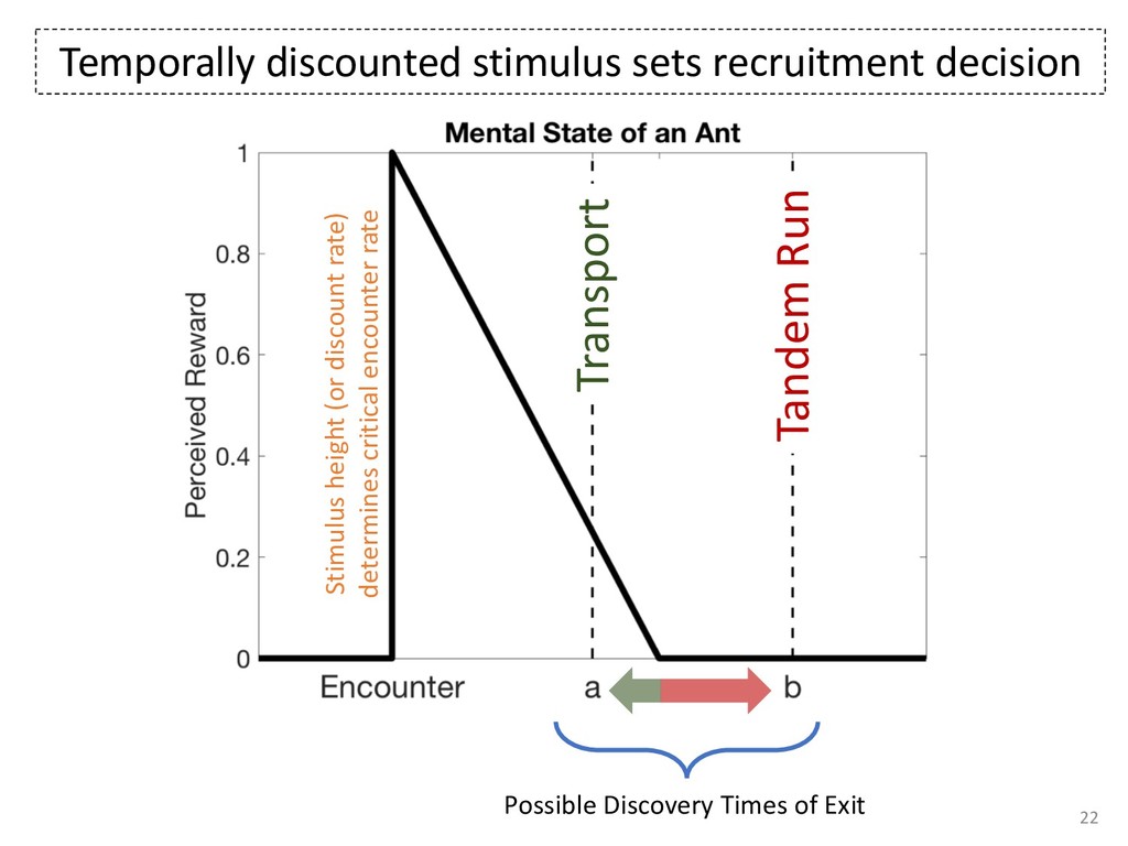
14. MODELING REACTION TIME 265 ned over the course of the exper- add to the payment rate for the he asterisks. They remained on the ich point the screen was erased. If iting period ensued and then the d. If the response was in error, the on the screen for 500 ms, followed of 50 trials was completed in less he subject was encouraged to take 11 sessions (except Subject 1, who mately 3 weeks. Each session was hin a block, one half of the stimuli and one half were sampled from of 1,200 observations per session used in any analysis (except for observations per subject. The first rded from the analyses. rials with response times less 00 ms were discarded (these . dividual differences in perfor- e long reaction times (in the ced very short reaction times other two were intermediate. ange of behaviors is a positive the models to have flexibility. , they might fit average data l data of the more extreme vided into three parts. First, it bjects' high and low responses the probabilities high and low showed sequential effects with ected by the response on the enerally slowed as the number er the crossover point between ross subjects, the relationship times varied. Third, the distri- the typical skewed shape and n either reached asymptote or asks; see Luce, 1986). ntial effects. Figure 1 shows r each subject as a function of vious response. The probabil- d they cross the 50th percentile hich the low and high distribu- performed without systematic l effects. For Subjects 1 and 4, S Q_ 0.0 Subject 1 0.6 0.0 • Subject 3 20 60 20 60 0.0 Subject 2 0.6 - 0.0 - 20 60 Number of Asterisks 20 60 Number of Asterisks x=low prior feedback and low prior response o=high prior feedback and low prior response +=low prior feedback and high prior response »=high prior feedback and high prior response Figure 1. Probability of a low response for the four subjects in Experi- ment 1. models because the mechanism that produces sequential effects must be flexible enough to behave in opposite ways for different subjects. The fact that sequential effects were dependent on the prior response and not on prior feedback is consistent with most earlier findings with psychophysical tasks (Thomas, 1973, 1975; Treis- man & Williams, 1984) and choice reaction time (Falmagne, Cohen, & Dwivedi, 1975; see Luce, 1986, chap. 7), although some studies, particularly in absolute identification (Ward & Lockhead, 1970), did find that feedback affected response probability. In the earliest investigations of signal detection paradigms, it appeared originally that any explanation of learning would have to take prior feedback into account (e.g., Kac, 1962), but Thomas (1973, 1975) showed that learning could be modeled by assuming criterion shifts toward the presented stimulus value so that learning did not depend directly on prior feedback. Thomas's account could also deal with paradigms in which feedback was not presented to the subject. Our experimental results are consistent with these early signal detection results and with the choice reaction-time results. Subjects knew that feedback was inconsistent and that for most stimuli the correct response was sometimes high and sometimes low. This, along with the large number of sessions tested per (Pavlic and Pratt, in prep) 266 RATCLIFF, VAN ZANDT, AND McKOON 700 500 350 20 60 20 60 600 300- 340 300 20 60 Number of Asterisks 20 60 Number of Asterisks +="low" responses x="high" responses Figure 2. Mean reaction time (RT) for the four subjects in Experiment 1. high and low responses. Generally, responses slowed as they neared the crossover point. For purposes of exposition, we defined error responses accord- ing to the crossover point (47); low responses to numbers greater than 47 are labeled errors, and so are high responses to numbers less than 47. We used error as the label for these responses because it is a convenient way of describing them. A response of this type is not exactly an error, but neither is it the best response because it is less likely to be correct than the alternative. (Note that this definition does not correspond to the feedback that was given subjects; ERROR -1 POINT feedback was determined by the distribution from which a number was drawn, not by its position relative to the crossover point.) We use the error terminology for compactness of description throughout this article. The subjects showed different patterns of error versus correct response times. For Subjects 1 and 2, errors for extreme stimulus numbers (e.g., numbers above 80 or below 20) were faster than correct responses for those numbers, whereas less extreme errors were slower than correct responses. But for Subject 4, errors were always faster than correct responses, and for Subject 3 errors were always slower than correct responses. This difference among sub- collapsed. So, for example asterisks can be averaged w equivalent high responses low response to 27 asteris of a high response to 67 a can be plotted against the in Figure 3. Thus, the late a parametric plot where th stimulus difficulty. The different patterns show up in the degree to are symmetric. Errors gene probability less than .5. corresponds to an error example, if the probability sponding error probability corresponding errors had probability function wou function with a maximum is asymmetric, with errors correct responses (see Fig tions are asymmetric, wit except that the most extr sponses. For Subject 4, t errors are a little faster th Besides providing a sum response probability functi traditional sequential samp Pike, 1965; Vickers, 1979 simple random walk m 550 i 15 So maybe dueling counters and thresholds are involved in setting the adaptive sampling period?
15. Does the process have to be cognitive at the level of an individual? 16
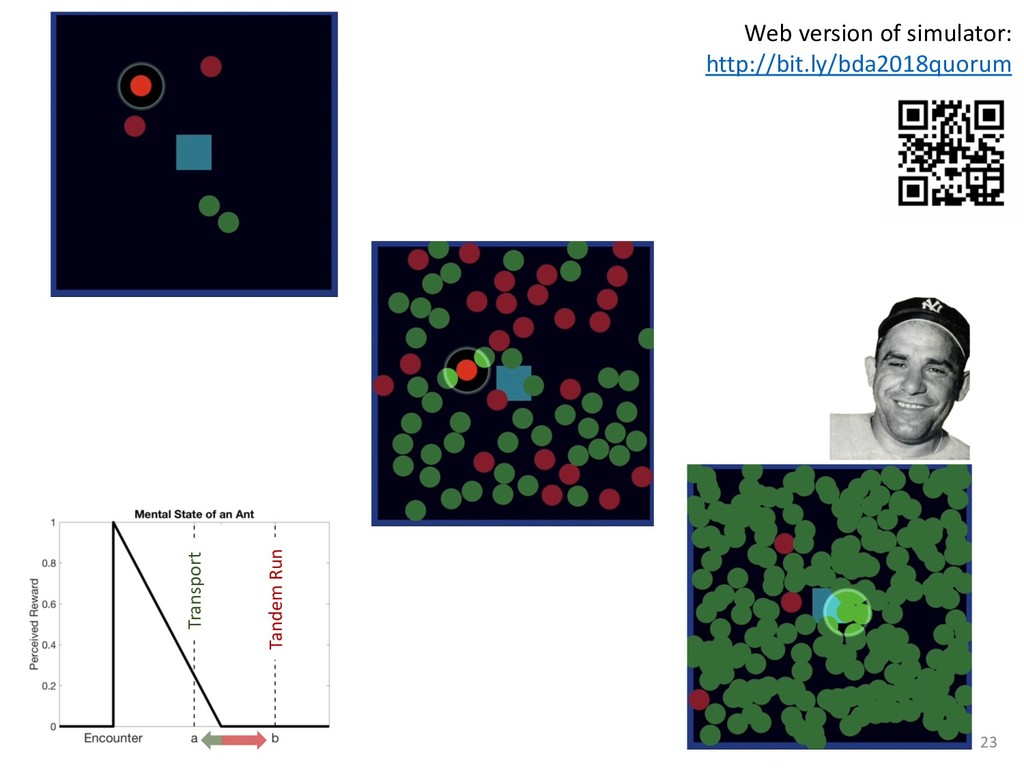
16. 17 Observed decision latency is exactly what is expected from a naïve 2D random walk amongst hard spheres.
17. 18 Empty Cavity 2D Brownian Recurrence Time Intermediate Packing Brownian Recurrence Time for >2 Fractal Dimension Tight Packing 1D Brownian Recurrence Time then Low Penetration Depth Sampling period is set by physical space. “Nobody goes there anymore. It’s too crowded.” “Nobody goes there anymore. It’s too crowded.”
18. Sampling period is set by physical space. An encounter is likely shortly before exit What if the natural discovery of exit forces the decision? An encounter is likely long before exit Tandem Run Transport 19
19. 189 _ in nectar delivery area * receives nectar from forager oinspects cell HIVE EMPTY OF HONEY w[ out of nectar delivery area 4 offers nectar to nestmate *deposits nectar in cell * fans 88. 4o* *o8 8 ?8 _ oS * 88o 80 *8 8 e cleanscell 4 *o * + 0 5 10 15 20 25 30 fans*0. o* 30 35 40 45 50 55 60 HIVE NEARLY FULL OF HONEY 0 0 * o O o00 8o o 0U concentrates nectar Uo U oI 8 oo,88 ; U 0 5 10 15 20 25 30 8o 8 04 ,o 8 ~ ~8 o , ~ 4, 84, 4 4 o44oo pollen * A+ * * * crawlsoutof hive outside 30 35 40 45 50 55 60 Time elapsed si Fig. 6. Typical tim bees when their h that the food sto area and the nect A more detailed view of the behavior of food storer bees reveals that their behavior is str influenced by the number of empty stora (Seeley, 1989, BES) Social foraging in honey bees: how nectar foragers assess their colony's nutritional st Thomas D. Seeley Section of Neurobiology and Behavior, Mudd Hall, Cornell University, Ithaca, NY 14853, USA Received June 8, 1988 / Accepted November 23, 1988 Summary. A honey bee colony operates as a tightly integrated unit of behavioral action. One manifes- tation of this in the context of foraging is a col- ony's ability to adjust its selectivity among nectar sources in relation to its nutritional status. When a colony's food situation is good, it exploits only highly profitable patches of flowers, but when its situation is poor, a colony's foragers will exploit both highly profitable and less profitable flower patches. The nectar foragers in a colony acquire information about their colony's nutritional status by noting the difficulty of finding food storer bees to receive their nectar, rather than by evaluating directly the variables determining their colony's food situation: rate of nectar intake and amount of empty storage comb. (The food storer bees in a colony are the bees that collect nectar from re- turning foragers and store it in the honey combs. They are the age group (generally 12-18 day old bees) that is older than the nurse bees but younger than the foragers. Food storers make up approxi- mately 20% of a colony members.) The mathemat- ical theory for the behavior of queues indicates that the waiting time experienced by nectar for- agers before unloading to food storers (queue length) is a reliable and sensitive indicator of a colony's nutritional status. Queue length is au- tomatically determined by the ratio of two rates which are directly related to a colony's nutritional condition: the rate of arrival of loaded nectar for- agers at the hive (arrival rate) and the rate of arriv- "cue" conveys information as an automatic by- product. Such cues may prove more important than signals in colony integration. Introduction In advanced social insects - such as army ants, fungus-growing termites, and honey bees - in which the colonies consists of one queen and many thousands of sterile workers, natural selection is based mainly on differences in survival and repro- duction between colonies, rather than between in- dividuals within these colonies. This colony-level selection has propeled the evolution of highly elab- orate societies which function as tightly integrated units of behavioral action. For example, to collect its food, a colony of honey bees gathers informa- tion about flower patches in the surrounding coun- tryside, skillfully chooses among these patches to exploit selectively those that are most profitable, and swiftly shifts the foci of its foraging efforts in response to changes in the foraging opportuni- ties (Seeley 1986, 1987; Seeley and Levien 1987). This and other impressive forms of integrated be- havior at the colony level, which reflect complex division of labor and altruistic interactions among a colony's members (reviewed for the social insects in general by Wilson 1971, 1985; Brian 1983; Markl 1985) are very telling because they reveal Behavioral Ecology Behav Ecol Sociobiol (1989) 24:181-199 and Sociobiology ? Springer-Verlag 1989 Social foraging in honey bees: how nectar foragers assess their colony's nutrit Thomas D. Seeley Section of Neurobiology and Behavior, Mudd Hall, Cornell University, Ithaca, NY 14853, Received June 8, 1988 / Accepted November 23, 1988 Summary. A honey bee colony operates as a tightly integrated unit of behavioral action. One manifes- tation of this in the context of foraging is a col- ony's ability to adjust its selectivity among nectar sources in relation to its nutritional status. When a colony's food situation is good, it exploits only highly profitable patches of flowers, but when its situation is poor, a colony's foragers will exploit both highly profitable and less profitable flower patches. The nectar foragers in a colony acquire information about their colony's nutritional status by noting the difficulty of finding food storer bees to receive their nectar, rather than by evaluating directly the variables determining their colony's food situation: rate of nectar intake and amount "cue" conveys information as an automatic by- product. Such cues may prove more important than signals in colony integration. Introduction In advanced social insects - such as army ants, fungus-growing termites, and honey bees - in which the colonies consists of one queen and many thousands of sterile workers, natural selection is based mainly on differences in survival and repro- duction between colonies, rather than between in- dividuals within these colonies. This colony-level An encounter is likely shortly after entrance An encounter is likely long after entrance Recruit Do not recruit 20
20. An encounter is likely shortly after entrance An encounter is likely long after entrance Recruit Do not recruit An encounter is likely shortly before exit An encounter is likely long before exit Tandem Run Transport VOL. 82, No. 4 JULY 1975 Psychological Bulletin Copyright © 1975 by the American Psychological Association, Inc. Specious Reward: A Behavioral Theory of Impulsiveness and Impulse Control George Ainslie Massachusetts Mental Health Center, Boston In a choice among assured, familiar outcomes of behavior, impulsiveness is the choice of less rewarding over more rewarding alternatives. Discussions of impulsiveness in the literature of economics, sociology, social psychology, dynamic psychology and psychiatry, behavioral psychology, and "behavior therapy" are reviewed. 'Impulsiveness seems to be best accounted for by the hyberbolic curves that have been found to describe the decline in effectiveness of rewards as the rewards are delayed from the time of choice. Such curves predict a reliable change of choice between some alternative rewards as a function of time. This change of choice provides a rationale for the known kinds of impulse control and relates them to several hitherto perplexing phe- nomena: behavioral rigidity, time-out from positive reinforcement, willpower, self-reward, compulsive traits, projection, boredom, and the capacity of punish- ing stimuli to attract attention. This article takes up the question of why organisms, particularly human beings, often freely choose the poorer, smaller, or more disastrous of two alternative rewards even when they seem to be entirely familiar with the alternatives. I call this kind of choice impulsive, although the word has also been used for behavior that is simply unpremedi- tated. The question of impulsiveness is one of the oldest on record—it is, after all, the subject of the story of Adam and Eve. It recurs in Homer in the story of Ulysses and This article was prepared in conjunction with research supported by National Institute of Mental the Sirens. Millenia of philosophical ponder- ing and decades of scientific observation have left us with three rather poorly defined guesses about why people are so prone to this maladaptive behavior: 1. In seeming to obey impulses, people do not knowingly choose the poorer alternative but have not really learned the consequences of their behavior. Socrates said something like this. Those who hold this kind of theory prescribe education or "insight" as the cure for impulsiveness. 2. In obeying impulses, people know the consequences of their behavior but are im- pelled by some lower principle (the devil, Temporal discounting The perceived value of a reward/stimulus decreases with time since the event 21
21. Tandem Run Transport Possible Discovery Times of Exit Temporally discounted stimulus sets recruitment decision Stimulus height (or discount rate) determines critical encounter rate 22
22. Tandem Run Transport Web version of simulator: http://bit.ly/bda2018quorum 23
23. 0 0.05 0.1 0.15 0.2 Focal-Ant Average Encounter Rate at Exit 0 500 1000 1500 2000 2500 Time (simulation time steps) Time for Focal Ant to Leave Nest Tandem Runners Transporters 0 0.05 0.1 0.15 0.2 Focal-Ant Average Encounter Rate at Exit Tandem Run Transport Decision of Focal Ant When Leaving Tandem Runners Transporters Hill (exp=100.00, halfsat=0.061) Half-Saturation @ 0.061 Weak Stimulus (High Discount Rate) 24
24. Medium Stimulus (Medium Discount Rate) 0 0.05 0.1 0.15 0.2 Focal-Ant Average Encounter Rate at Exit 0 2000 4000 6000 8000 Time (simulation time steps) Time for Focal Ant to Leave Nest Tandem Runners Transporters 0 0.05 0.1 0.15 0.2 Focal-Ant Average Encounter Rate at Exit Tandem Run Transport Decision of Focal Ant When Leaving Tandem Runners Transporters Hill (exp=67.27, halfsat=0.038) Half-Saturation @ 0.038 25
25. Strong Stimulus (Low Discount Rate) 0 0.02 0.04 0.06 0.08 0.1 0.12 0.14 0.16 Focal-Ant Average Encounter Rate at Exit 0 1000 2000 3000 4000 5000 6000 Time (simulation time steps) Time for Focal Ant to Leave Nest Tandem Runners Transporters 0 0.02 0.04 0.06 0.08 0.1 0.12 0.14 0.16 Focal-Ant Average Encounter Rate at Exit Tandem Run Transport Decision of Focal Ant When Leaving Tandem Runners Transporters Hill (exp=1.81, halfsat=0.007) Half-Saturation @ 0.007 26
26. -nano robots could also generate such a pulse. A multi-robot system implementing TD-QS can be d event-triggered rules summarized by the chemical re S + S ea * 2R S + R ea * 2R S + E ee * XT R + E Theodore P. Pavlic et al. R + E ee * XT + E R 1/⌧ * S the CRN, a robot enters the confined space in the Tandem Run Transport …also amenable to theoretical analysis. 0 200 400 600 800 1000 Total Number of Ants in Nest 0 0.1 0.2 0.3 0.4 0.5 0.6 0.7 0.8 0.9 1 Equilibrium Fraction of Transporters in Nest 27
27. For take away… 28 • The ants are an interacting ensemble • The cavity’s physical space is a sampler • The computational model should be at the level of the ant–cavity system • More broadly: Physical spaces provide memory and even computational primitives for free
28. Dr. Sara Walker Dr. Stephen Pratt Jake Hanson 29 Dr. Gabriele Valentini Thanks to the BDA 2018 organizers! The Team: Acknowledgements: NSF PHY-1505048
29. 30 “Any questions?” @TedPavlic tpavlic@asu.edu Web version of simulator: http://bit.ly/bda2018quorum For More Information: “Any questions?” via guardian.co.uk “Any questions?”