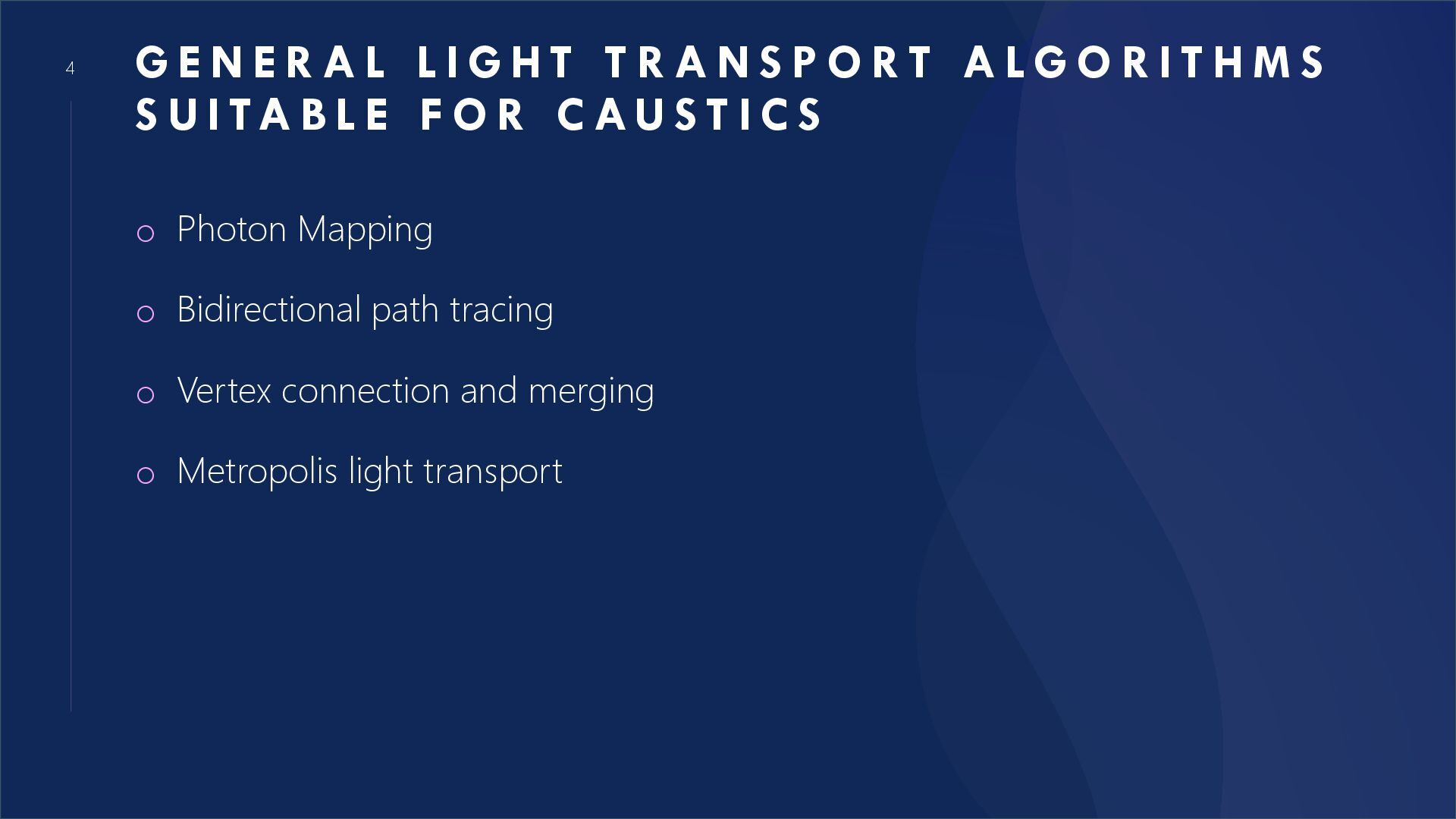
G H T T R A N S P O R T A L G O R I T H M S S U I TA B L E F O R C AU S T I C S o Photon Mapping o Bidirectional path tracing o Vertex connection and merging o Metropolis light transport
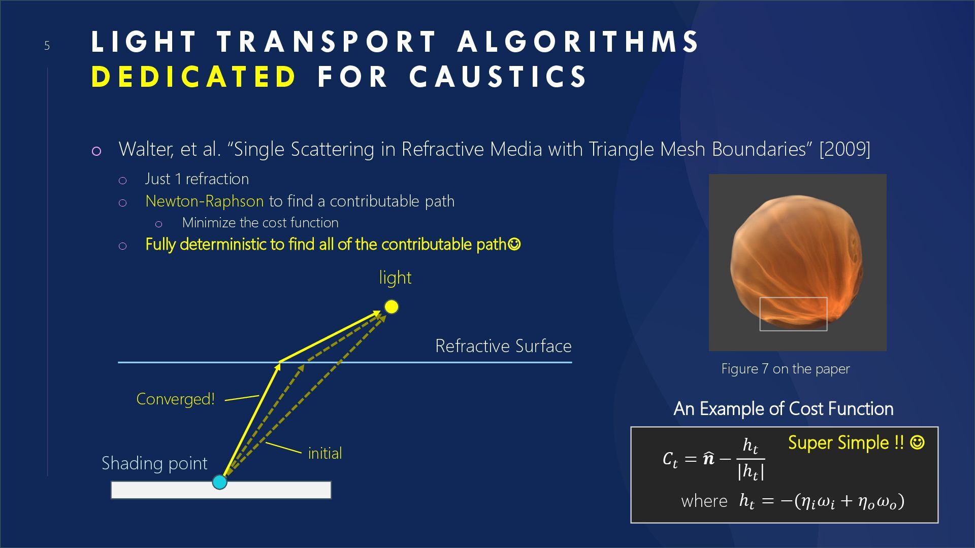
S P O R T A L G O R I T H M S D E D I C AT E D F O R C AU S T I C S o Walter, et al. “Single Scattering in Refractive Media with Triangle Mesh Boundaries” [2009] o Just 1 refraction o Newton-Raphson to find a contributable path o Minimize the cost function o Fully deterministic to find all of the contributable path☺ Figure 7 on the paper An Example of Cost Function 𝐶𝑡 = ෝ 𝒏 − ℎ𝑡 |ℎ𝑡 | ℎ𝑡 = −(𝜂𝑖 𝜔𝑖 + 𝜂𝑜 𝜔𝑜 ) where Super Simple !! ☺ light Refractive Surface Shading point initial Converged!
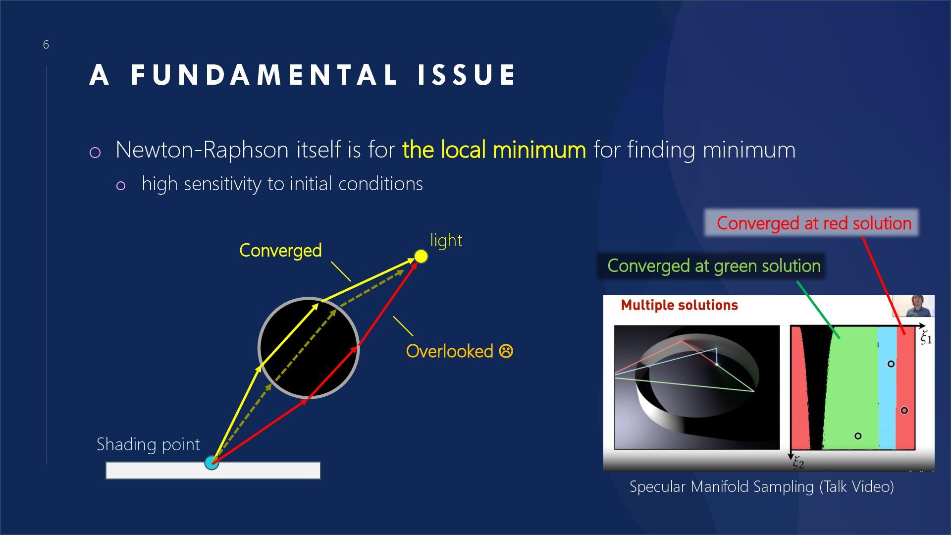
L I S S U E o Newton-Raphson itself is for the local minimum for finding minimum o high sensitivity to initial conditions Shading point light Converged Overlooked Specular Manifold Sampling (Talk Video) Converged at green solution Converged at red solution
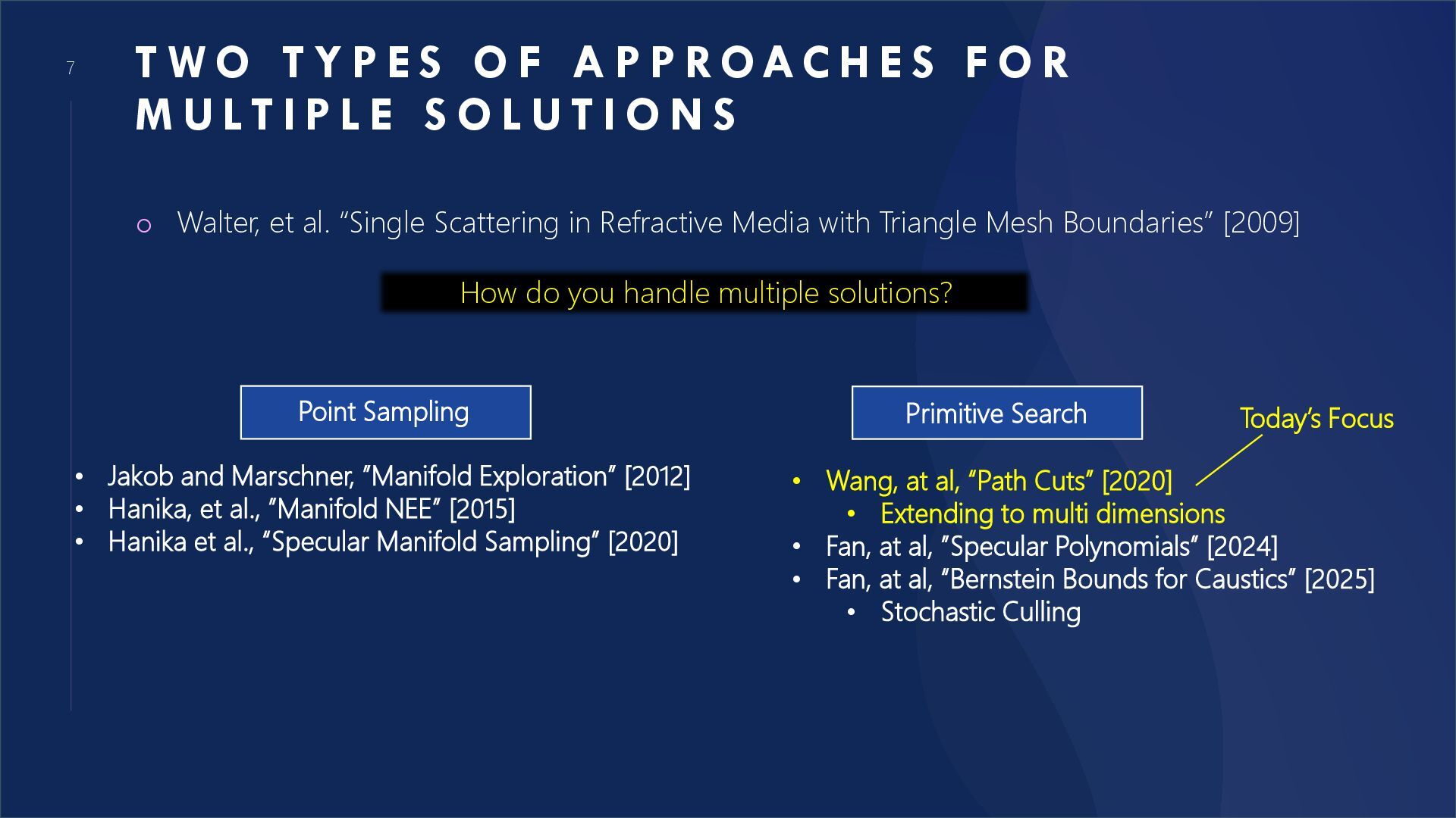
F A P P ROAC H E S F O R M U L T I P L E S O L U T I O N S o Walter, et al. “Single Scattering in Refractive Media with Triangle Mesh Boundaries” [2009] Point Sampling • Jakob and Marschner, ”Manifold Exploration” [2012] • Hanika, et al., ”Manifold NEE” [2015] • Hanika et al., “Specular Manifold Sampling” [2020] Primitive Search • Wang, at al, “Path Cuts” [2020] • Extending to multi dimensions • Fan, at al, ”Specular Polynomials” [2024] • Fan, at al, “Bernstein Bounds for Caustics” [2025] • Stochastic Culling Today’s Focus How do you handle multiple solutions?
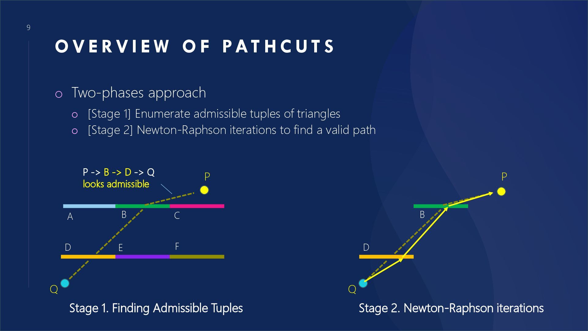
PAT H C U T S o Two-phases approach o [Stage 1] Enumerate admissible tuples of triangles o [Stage 2] Newton-Raphson iterations to find a valid path P P -> B -> D -> Q looks admissible D A B C E F Q Stage 1. Finding Admissible Tuples P D B Q Stage 2. Newton-Raphson iterations
N D I N G A D M I S S I B L E T U P L E S o Brute force search works, but prohibitively expensive o Search using a bounding volume hierarchy for mesh P Q Check if an admissible path is contained Yes P Q Go down the tree and do the same recursively Check this box too This can be seen as a cut of non-admissible path space. Path Cuts
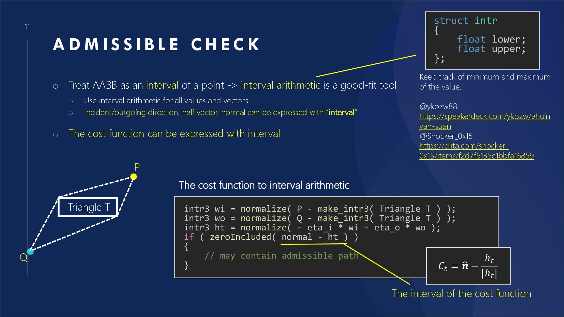
E C H E C K o Treat AABB as an interval of a point -> interval arithmetic is a good-fit tool o Use interval arithmetic for all values and vectors o Incident/outgoing direction, half vector, normal can be expressed with “interval” o The cost function can be expressed with interval struct intr { float lower; float upper; }; Keep track of minimum and maximum of the value. @ykozw88 https://speakerdeck.com/ykozw/ahuin yan-suan @Shocker_0x15 https://qiita.com/shocker- 0x15/items/f2d7f6135c1bbfa16859 P Q Triangle T The cost function to interval arithmetic intr3 wi = normalize( P - make_intr3( Triangle T ) ); intr3 wo = normalize( Q - make_intr3( Triangle T ) ); intr3 ht = normalize( - eta_i * wi - eta_o * wo ); if ( zeroIncluded( normal - ht ) ) { // may contain admissible path } The interval of the cost function 𝐶𝑡 = ෝ 𝒏 − ℎ𝑡 |ℎ𝑡 |
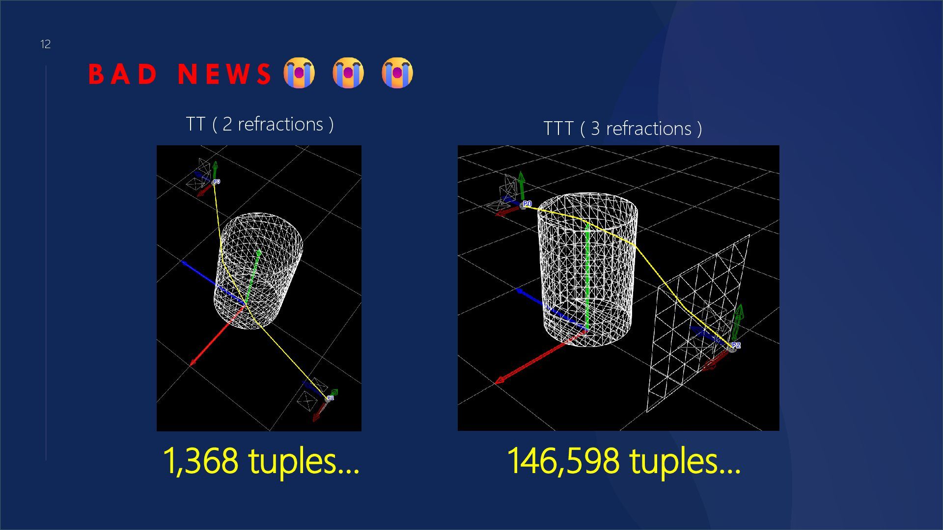
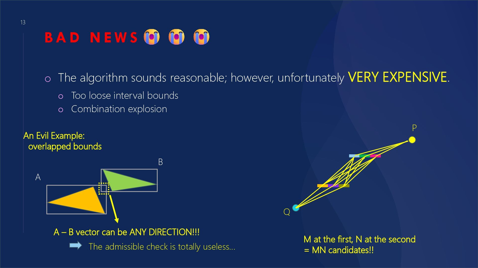
algorithm sounds reasonable; however, unfortunately VERY EXPENSIVE. o Too loose interval bounds o Combination explosion A B An Evil Example: overlapped bounds A – B vector can be ANY DIRECTION!!! The admissible check is totally useless… P Q M at the first, N at the second = MN candidates!!
E C A N D O ? o Specialize some functions interval arithmetic o Square, normalize, reflection, etc.. o Affine Arithmetic o Combination explosion still there..
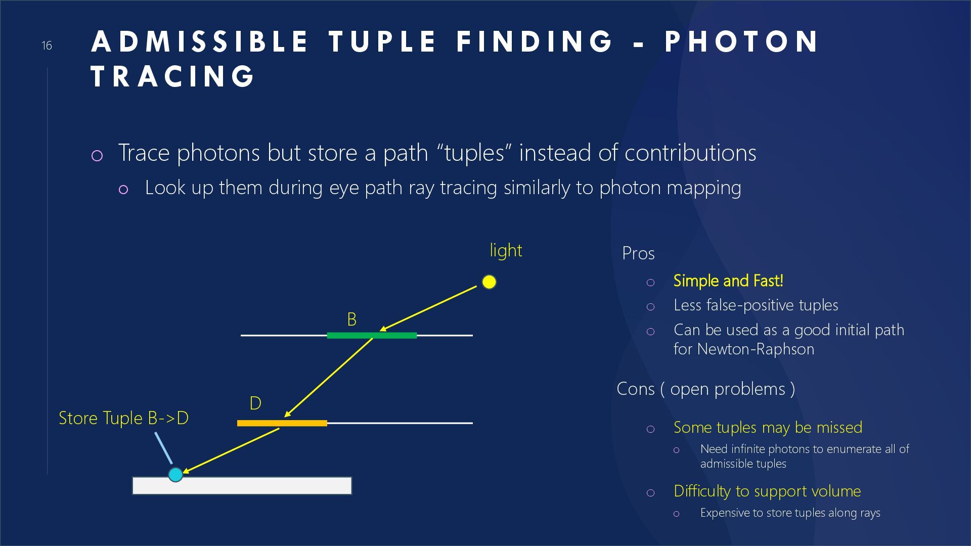
E T U P L E F I N D I N G - P H O T O N T R AC I N G o Trace photons but store a path “tuples” instead of contributions o Look up them during eye path ray tracing similarly to photon mapping light B D Store Tuple B->D Pros o Simple and Fast! o Less false-positive tuples o Can be used as a good initial path for Newton-Raphson Cons ( open problems ) o Some tuples may be missed o Need infinite photons to enumerate all of admissible tuples o Difficulty to support volume o Expensive to store tuples along rays
T F I N D I N G o Assumes there is only 1 solution for each tuple for simplicity o Assumes the scene geometry is subdivided enough o The resolution dependency is a weak point of primitive search algorithms o We can use subdivision but appropriate depth are not clear
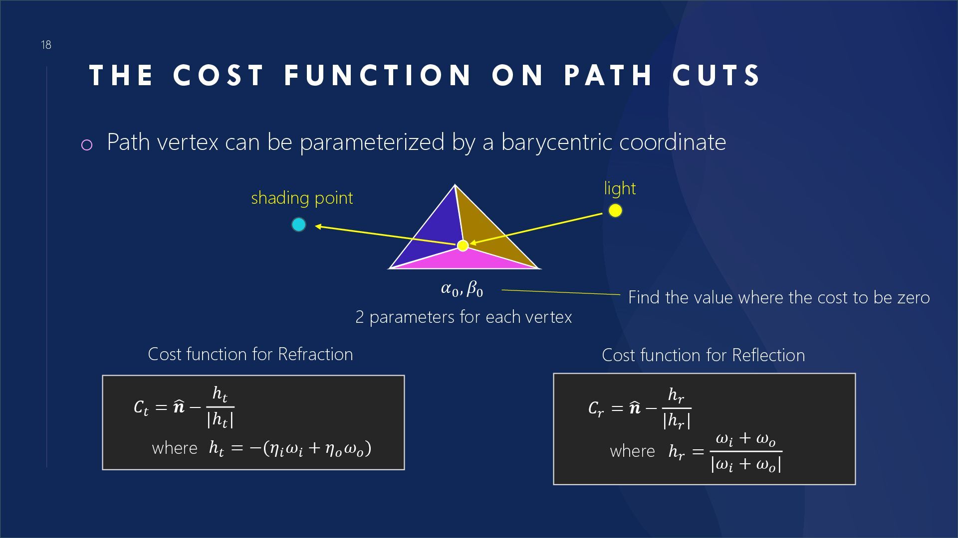
N C T I O N O N PAT H C U T S o Path vertex can be parameterized by a barycentric coordinate 𝐶𝑡 = ෝ 𝒏 − ℎ𝑡 |ℎ𝑡 | ℎ𝑡 = −(𝜂𝑖 𝜔𝑖 + 𝜂𝑜 𝜔𝑜 ) where Cost function for Refraction 𝐶𝑟 = ෝ 𝒏 − ℎ𝑟 |ℎ𝑟 | ℎ𝑟 = 𝜔𝑖 + 𝜔𝑜 |𝜔𝑖 + 𝜔𝑜 | where Cost function for Reflection light shading point 𝛼0 , 𝛽0 2 parameters for each vertex Find the value where the cost to be zero
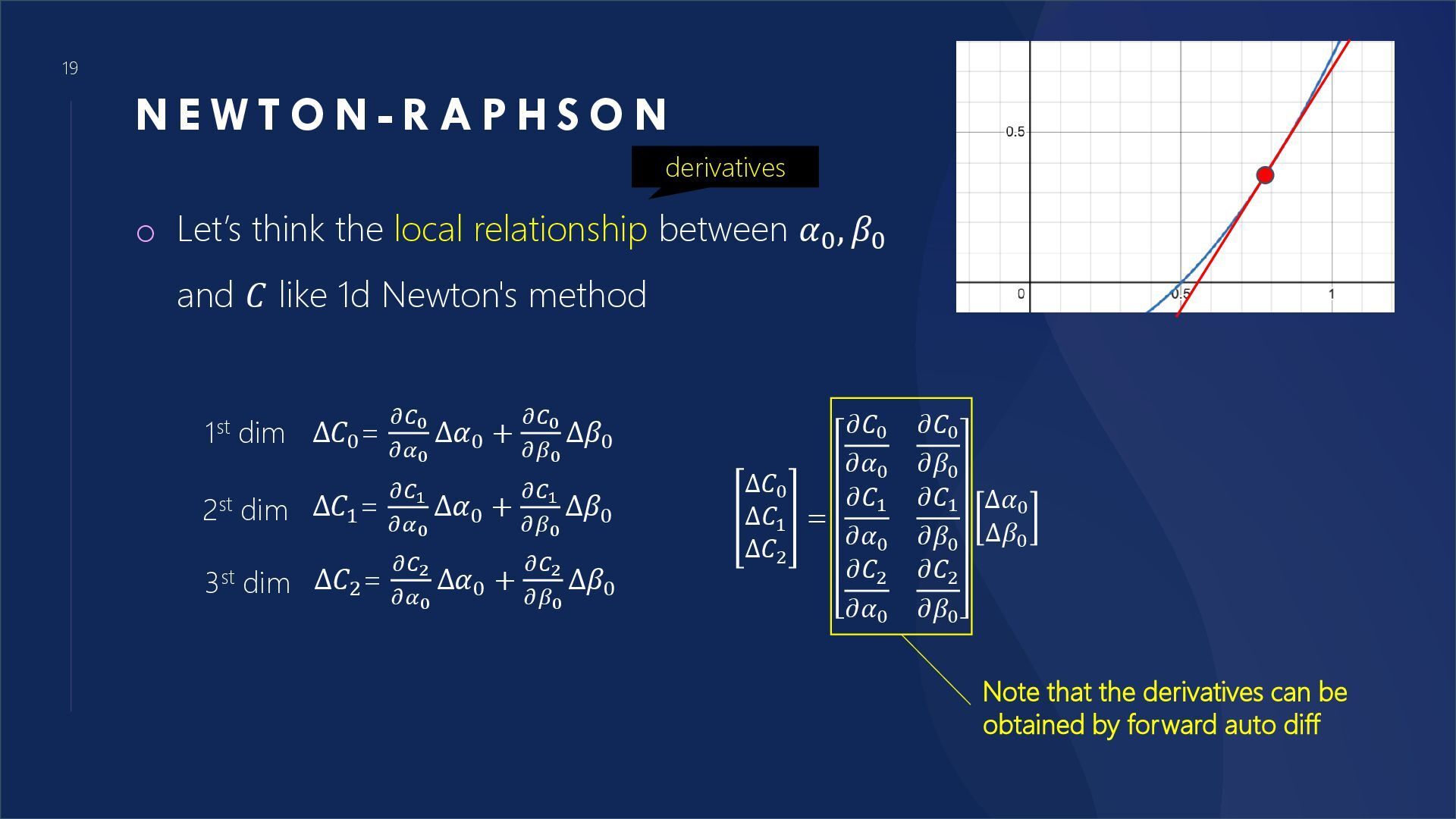
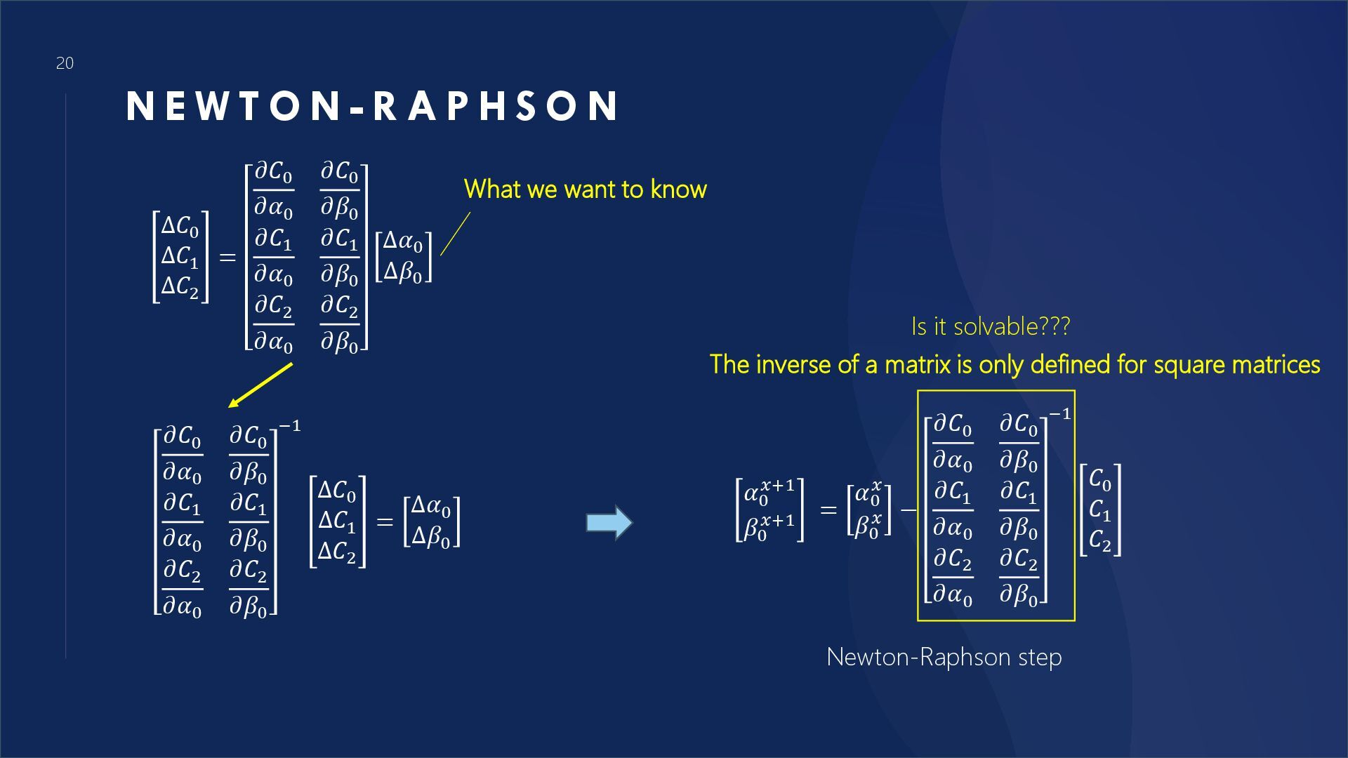
P H S O N o Let’s think the local relationship between 𝛼0 , 𝛽0 and 𝐶 like 1d Newton's method Δ𝐶0 Δ𝐶1 Δ𝐶2 = 𝜕𝐶0 𝜕𝛼0 𝜕𝐶0 𝜕𝛽0 𝜕𝐶1 𝜕𝛼0 𝜕𝐶1 𝜕𝛽0 𝜕𝐶2 𝜕𝛼0 𝜕𝐶2 𝜕𝛽0 Δ𝛼0 Δ𝛽0 Δ𝐶0= 𝜕𝐶0 𝜕𝛼0 Δ𝛼0 + 𝜕𝐶0 𝜕𝛽0 Δ𝛽0 1st dim Δ𝐶1= 𝜕𝐶1 𝜕𝛼0 Δ𝛼0 + 𝜕𝐶1 𝜕𝛽0 Δ𝛽0 2st dim Δ𝐶2= 𝜕𝐶2 𝜕𝛼0 Δ𝛼0 + 𝜕𝐶2 𝜕𝛽0 Δ𝛽0 3st dim Note that the derivatives can be obtained by forward auto diff derivatives
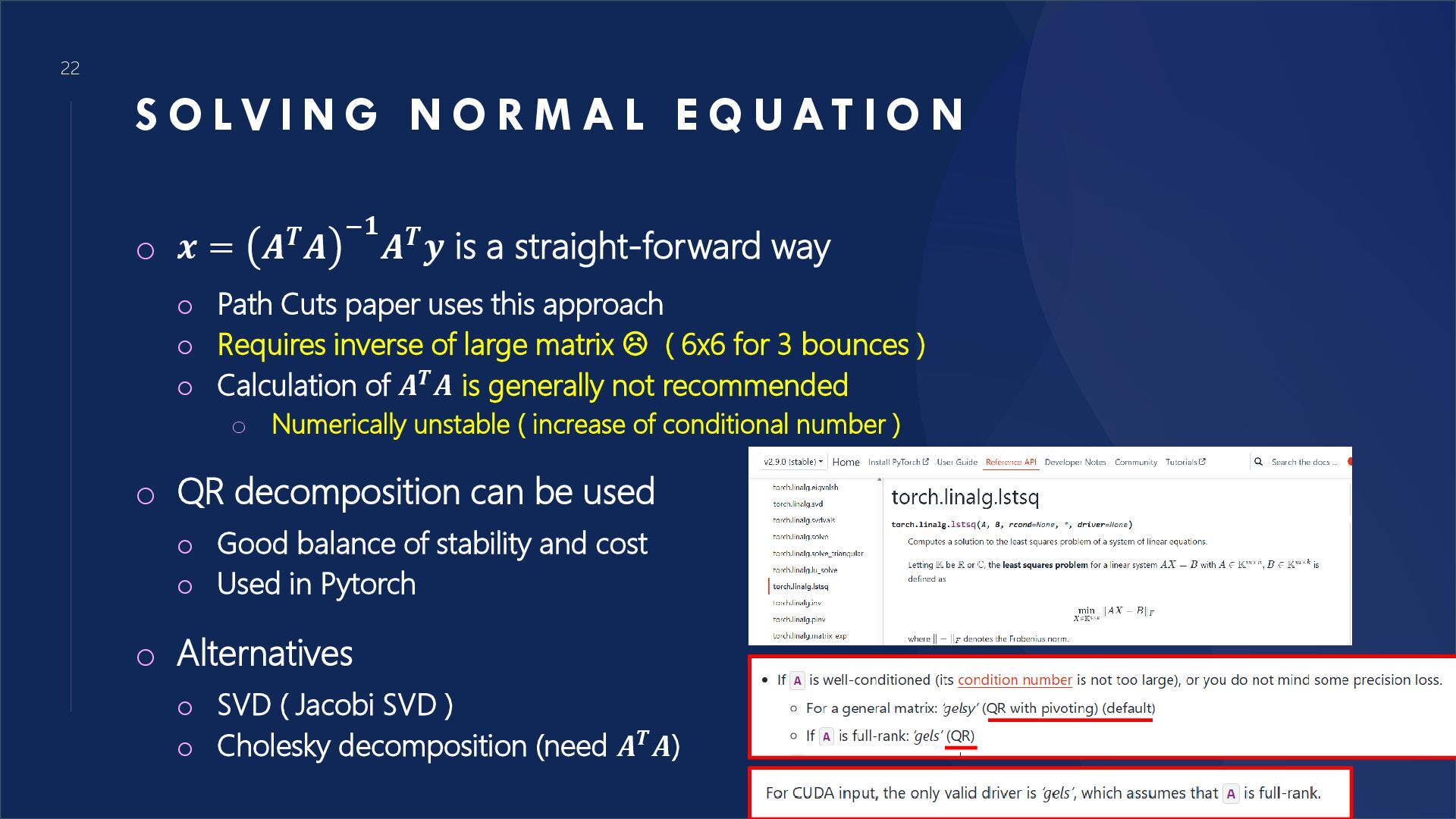
M A L E Q U AT I O N o 𝒙 = 𝑨𝑻𝑨 −𝟏 𝑨𝑻𝒚 is a straight-forward way o Path Cuts paper uses this approach o Requires inverse of large matrix ( 6x6 for 3 bounces ) o Calculation of 𝑨𝑻𝑨 is generally not recommended o Numerically unstable ( increase of conditional number ) o QR decomposition can be used o Good balance of stability and cost o Used in Pytorch o Alternatives o SVD ( Jacobi SVD ) o Cholesky decomposition (need 𝑨𝑻𝑨)
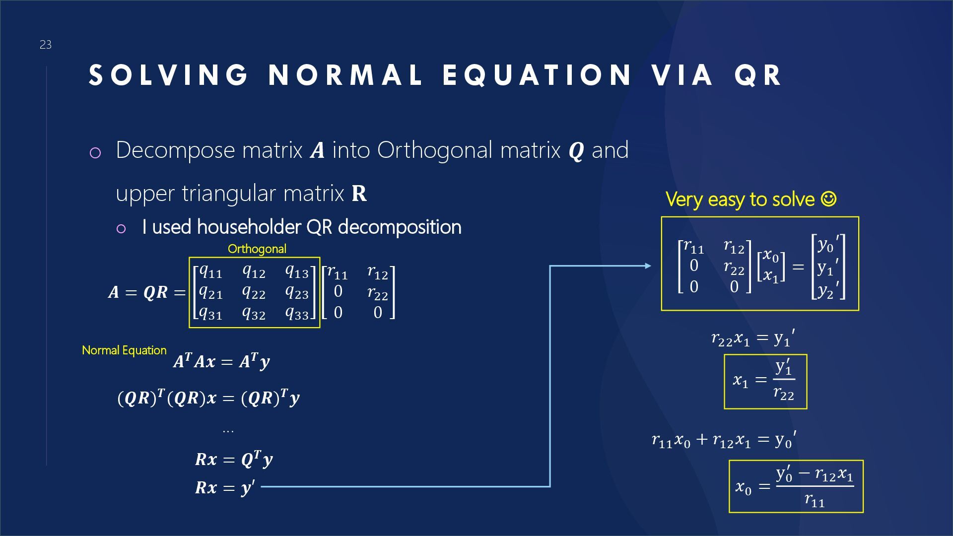
M A L E Q U AT I O N V I A Q R o Decompose matrix 𝑨 into Orthogonal matrix 𝑸 and upper triangular matrix 𝐑 o I used householder QR decomposition (𝑸𝑹)𝑻(𝑸𝑹)𝒙 = (𝑸𝑹)𝑻𝒚 𝑹𝒙 = 𝑸𝑻𝒚 … 𝑹𝒙 = 𝒚′ 𝑟11 𝑟12 0 𝑟22 0 0 𝑥0 𝑥1 = 𝑦0 ′ y1 ′ 𝑦2 ′ Very easy to solve ☺ 𝑟11 𝑥0 + 𝑟12 𝑥1 = y0 ′ 𝑥0 = y0 ′ − 𝑟12 𝑥1 𝑟11 𝑨𝑻𝑨𝒙 = 𝑨𝑻𝒚 Normal Equation 𝑨 = 𝑸𝑹 = 𝑞11 𝑞12 𝑞13 𝑞21 𝑞22 𝑞23 𝑞31 𝑞32 𝑞33 𝑟11 𝑟12 0 𝑟22 0 0 Orthogonal 𝑥1 = y1 ′ 𝑟22 𝑟22 𝑥1 = y1 ′
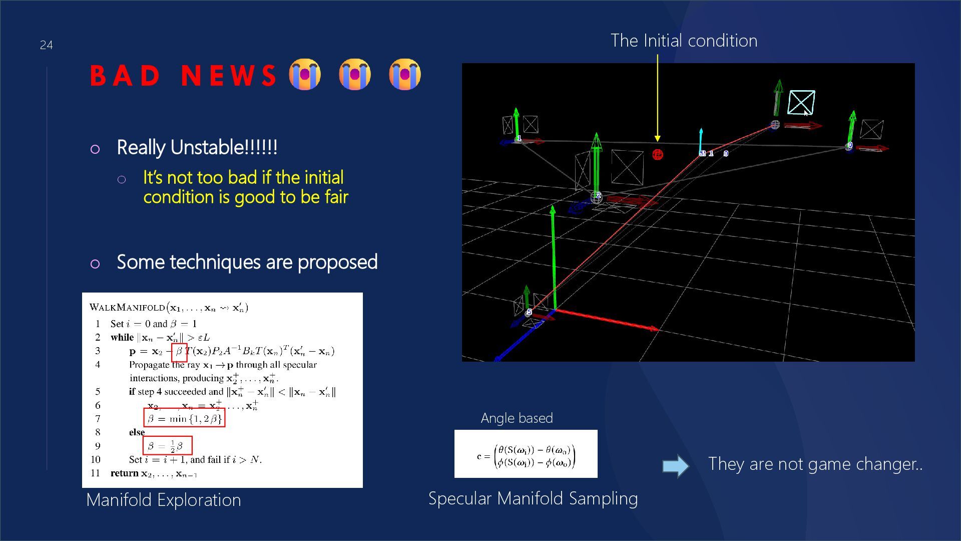
Unstable!!!!!! o It’s not too bad if the initial condition is good to be fair o Some techniques are proposed The Initial condition Manifold Exploration Specular Manifold Sampling Angle based They are not game changer..
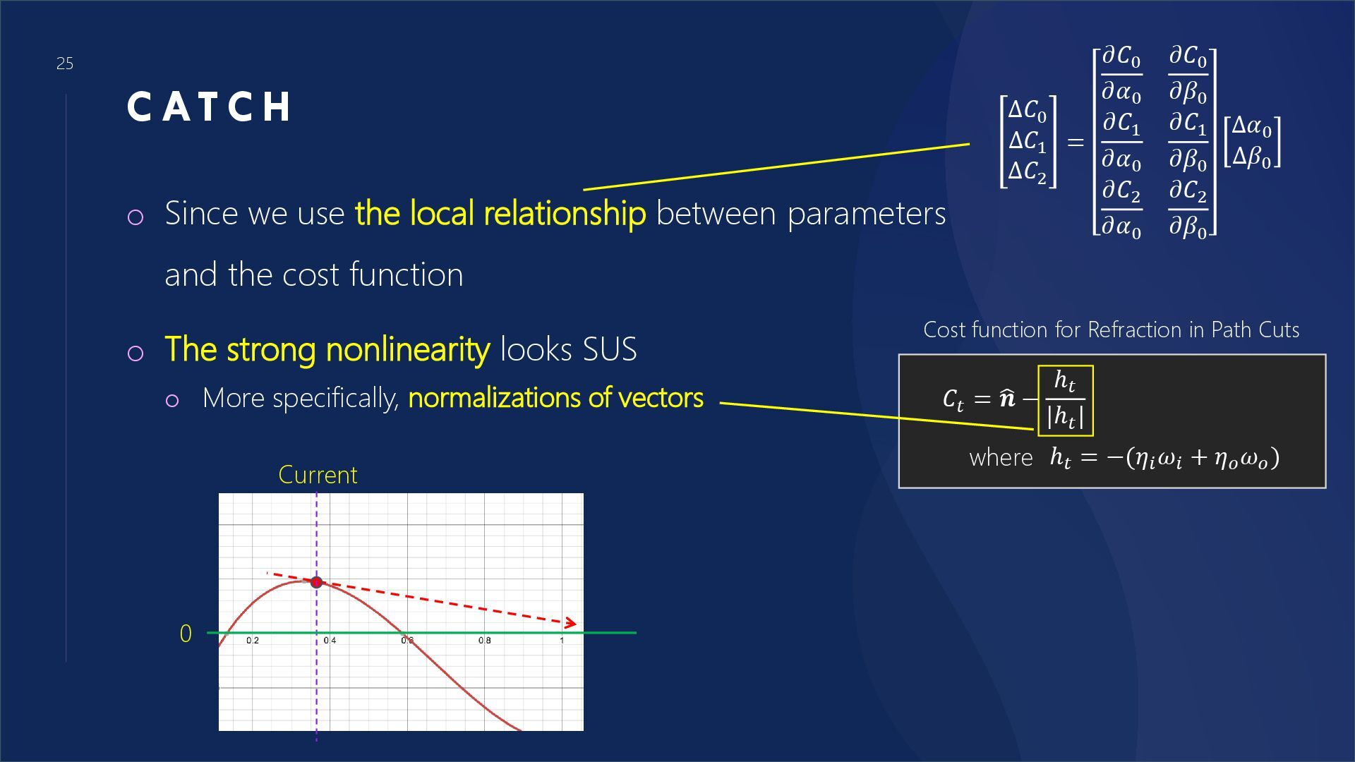
local relationship between parameters and the cost function o The strong nonlinearity looks SUS o More specifically, normalizations of vectors Δ𝐶0 Δ𝐶1 Δ𝐶2 = 𝜕𝐶0 𝜕𝛼0 𝜕𝐶0 𝜕𝛽0 𝜕𝐶1 𝜕𝛼0 𝜕𝐶1 𝜕𝛽0 𝜕𝐶2 𝜕𝛼0 𝜕𝐶2 𝜕𝛽0 Δ𝛼0 Δ𝛽0 𝐶𝑡 = ෝ 𝒏 − ℎ𝑡 |ℎ𝑡 | ℎ𝑡 = −(𝜂𝑖 𝜔𝑖 + 𝜂𝑜 𝜔𝑜 ) where Cost function for Refraction in Path Cuts Current 0
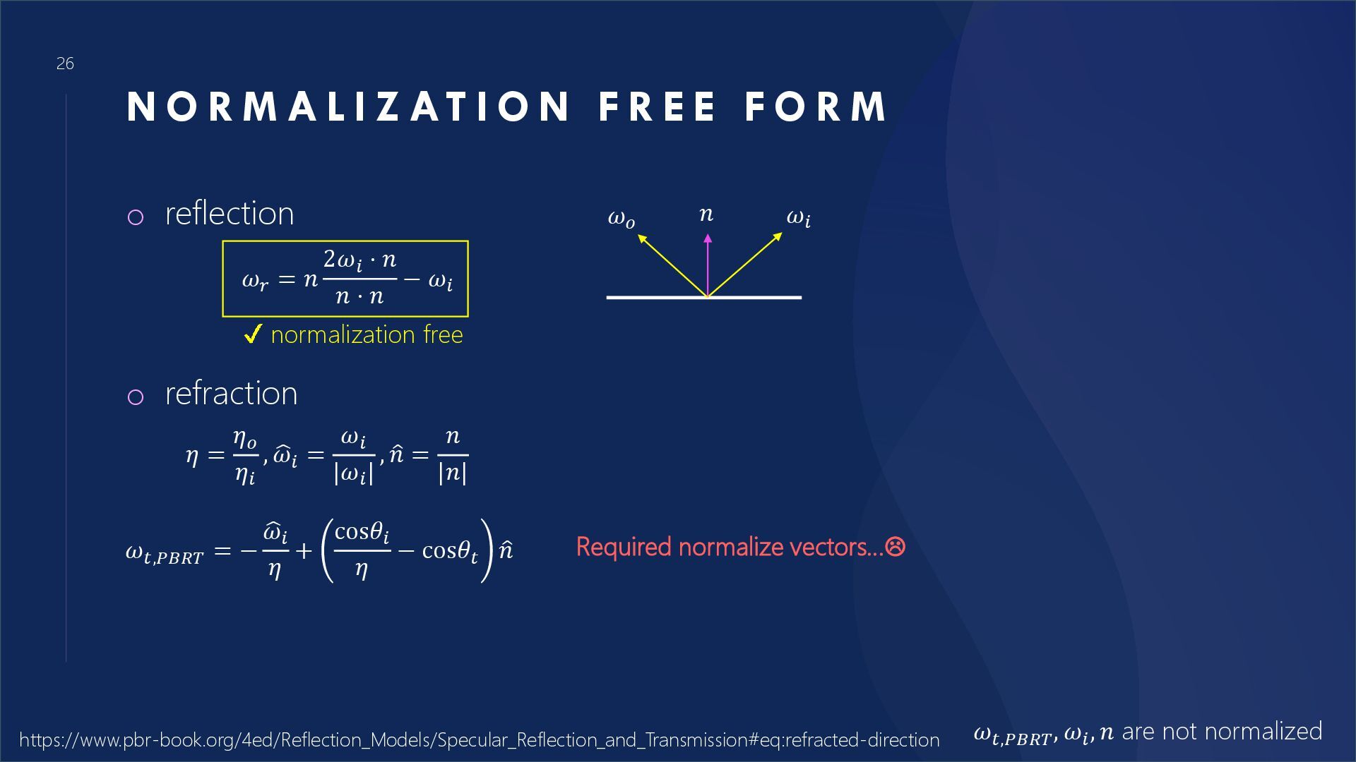
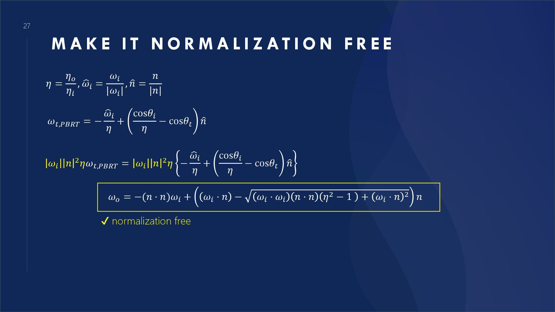
I O N F R E E F O R M o reflection 𝜔𝑟 = 𝑛 2𝜔𝑖 ⋅ 𝑛 𝑛 ⋅ 𝑛 − 𝜔𝑖 𝜔𝑖 𝑛 𝜔𝑜 normalization free o refraction 𝜔𝑡,𝑃𝐵𝑅𝑇 = − ෝ 𝜔𝑖 𝜂 + cos𝜃𝑖 𝜂 − cos𝜃𝑡 ො 𝑛 𝜔𝑡,𝑃𝐵𝑅𝑇 , 𝜔𝑖 , 𝑛 are not normalized 𝜂 = 𝜂𝑜 𝜂𝑖 , ෝ 𝜔𝑖 = 𝜔𝑖 |𝜔𝑖 | , ො 𝑛 = 𝑛 |𝑛| Required normalize vectors… https://www.pbr-book.org/4ed/Reflection_Models/Specular_Reflection_and_Transmission#eq:refracted-direction
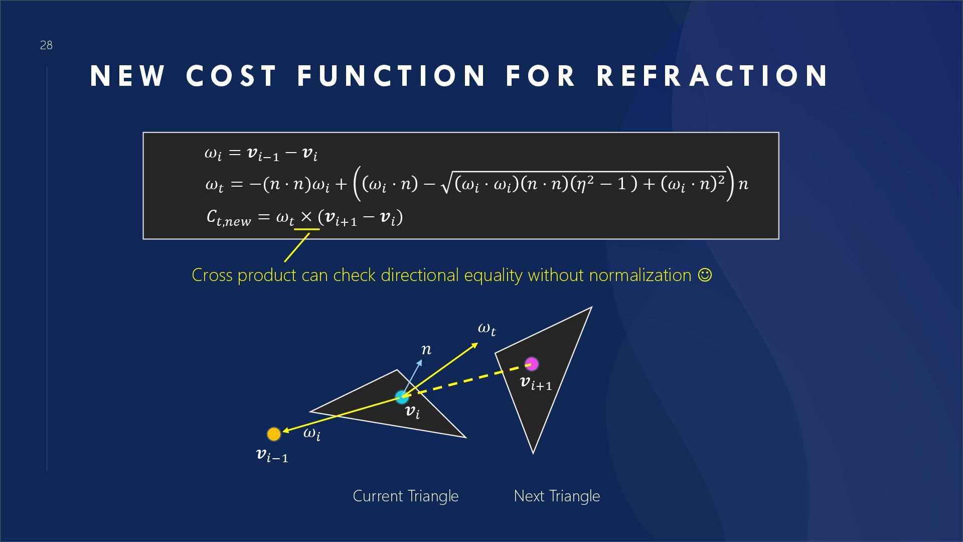
N C T I O N F O R R E F R AC T I O N 𝐶𝑡,𝑛𝑒𝑤 = 𝜔𝑡 × (𝒗𝑖+1 − 𝒗𝑖 ) 𝜔𝑡 𝒗𝑖 𝒗𝑖+1 Next Triangle Current Triangle 𝜔𝑖 𝜔𝑖 = 𝒗𝑖−1 − 𝒗𝑖 𝒗𝑖−1 𝑛 𝜔𝑡 = −(𝑛 ⋅ 𝑛)𝜔𝑖 + 𝜔𝑖 ⋅ 𝑛 − 𝜔𝑖 ⋅ 𝜔𝑖 𝑛 ⋅ 𝑛 𝜂2 − 1 + 𝜔𝑖 ⋅ 𝑛 2 𝑛 Cross product can check directional equality without normalization ☺
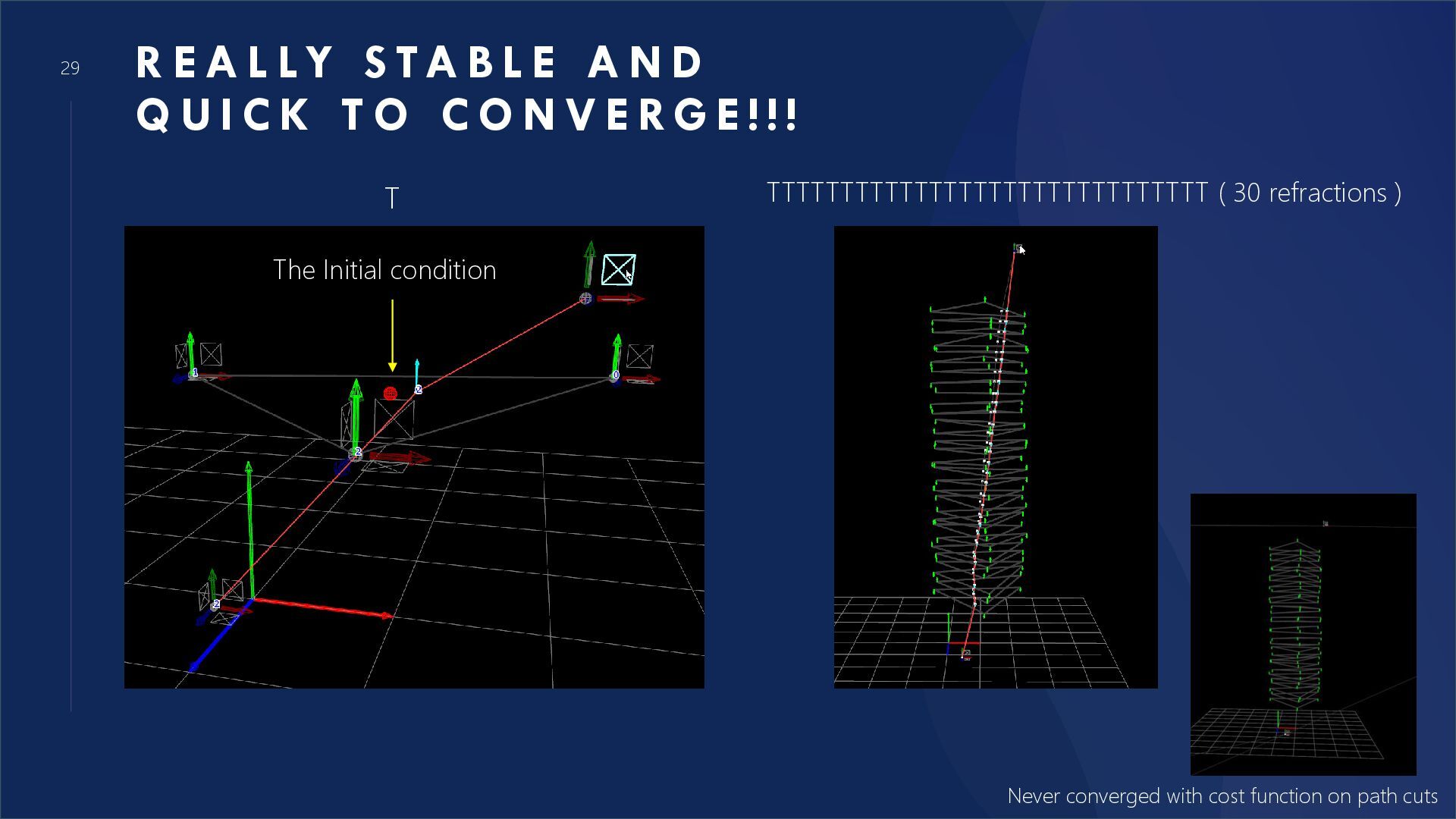
E A N D Q U I C K T O C O N V E R G E ! ! ! T Never converged with cost function on path cuts TTTTTTTTTTTTTTTTTTTTTTTTTTTTTT ( 30 refractions ) The Initial condition
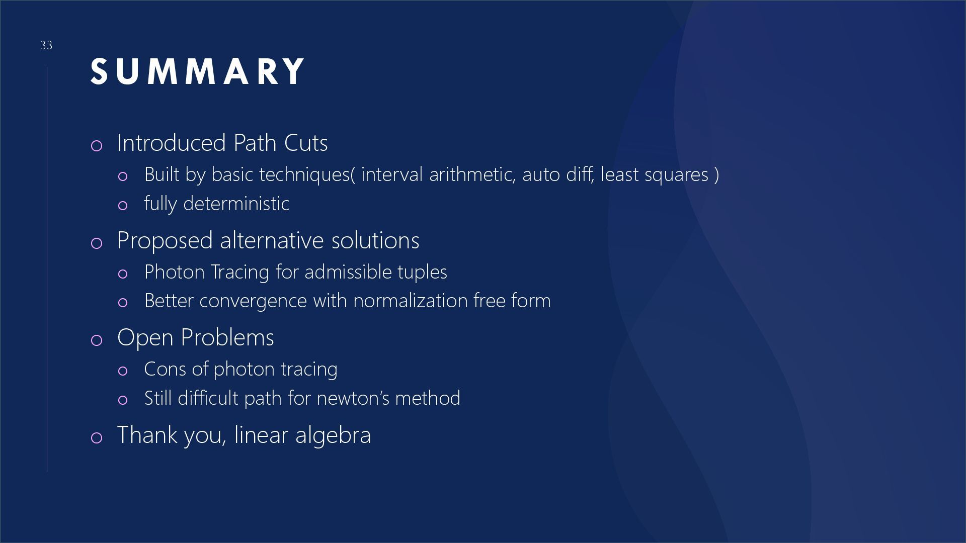
basic techniques( interval arithmetic, auto diff, least squares ) o fully deterministic o Proposed alternative solutions o Photon Tracing for admissible tuples o Better convergence with normalization free form o Open Problems o Cons of photon tracing o Still difficult path for newton’s method o Thank you, linear algebra
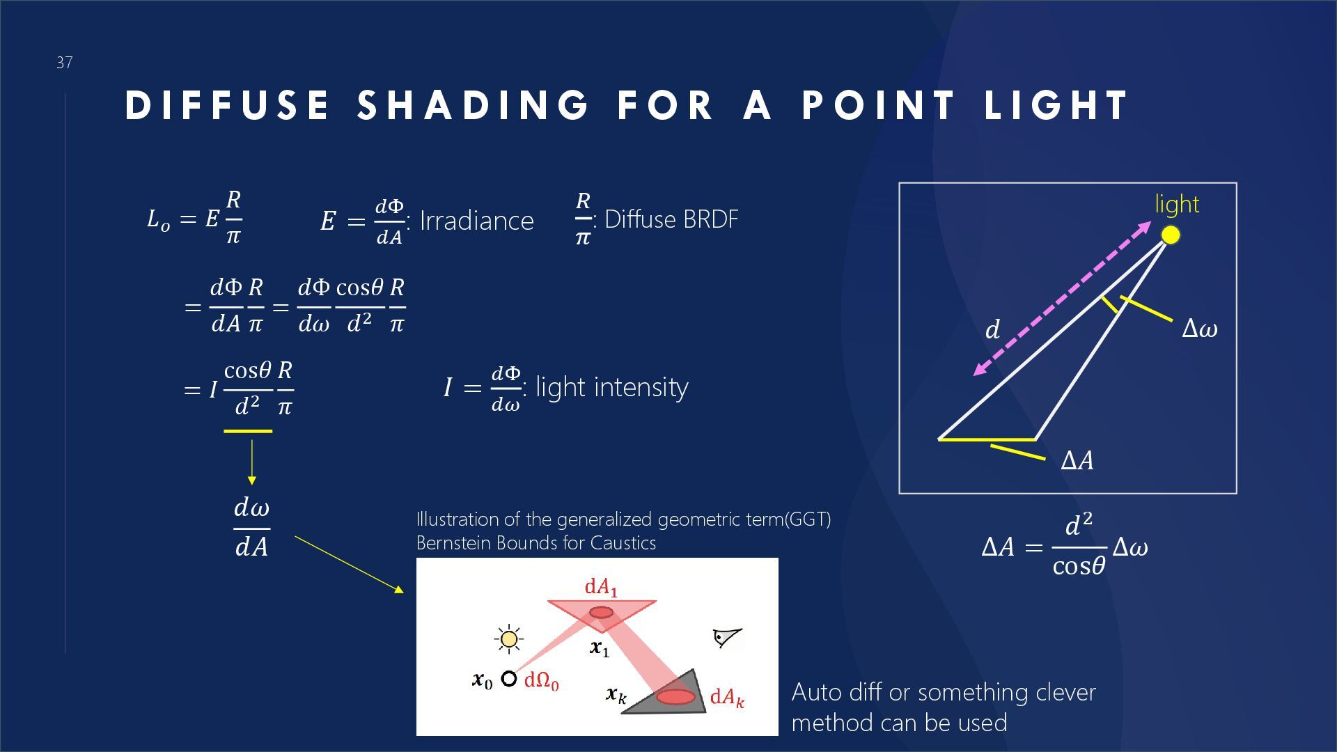
A D I N G F O R A P O I N T L I G H T Illustration of the generalized geometric term(GGT) Bernstein Bounds for Caustics 𝐿𝑜 = 𝐸 𝑅 𝜋 𝐸 = 𝑑Φ 𝑑𝐴 : Irradiance 𝑅 𝜋 : Diffuse BRDF light Δ𝜔 Δ𝐴 = 𝑑2 cos𝜃 Δ𝜔 𝑑 Δ𝐴 = 𝑑Φ 𝑑𝐴 𝑅 𝜋 = 𝑑Φ 𝑑𝜔 cos𝜃 𝑑2 𝑅 𝜋 = 𝐼 cos𝜃 𝑑2 𝑅 𝜋 𝐼 = 𝑑Φ 𝑑𝜔 : light intensity 𝑑𝜔 𝑑𝐴 Auto diff or something clever method can be used
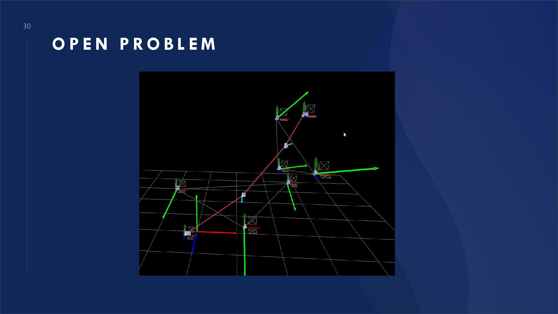
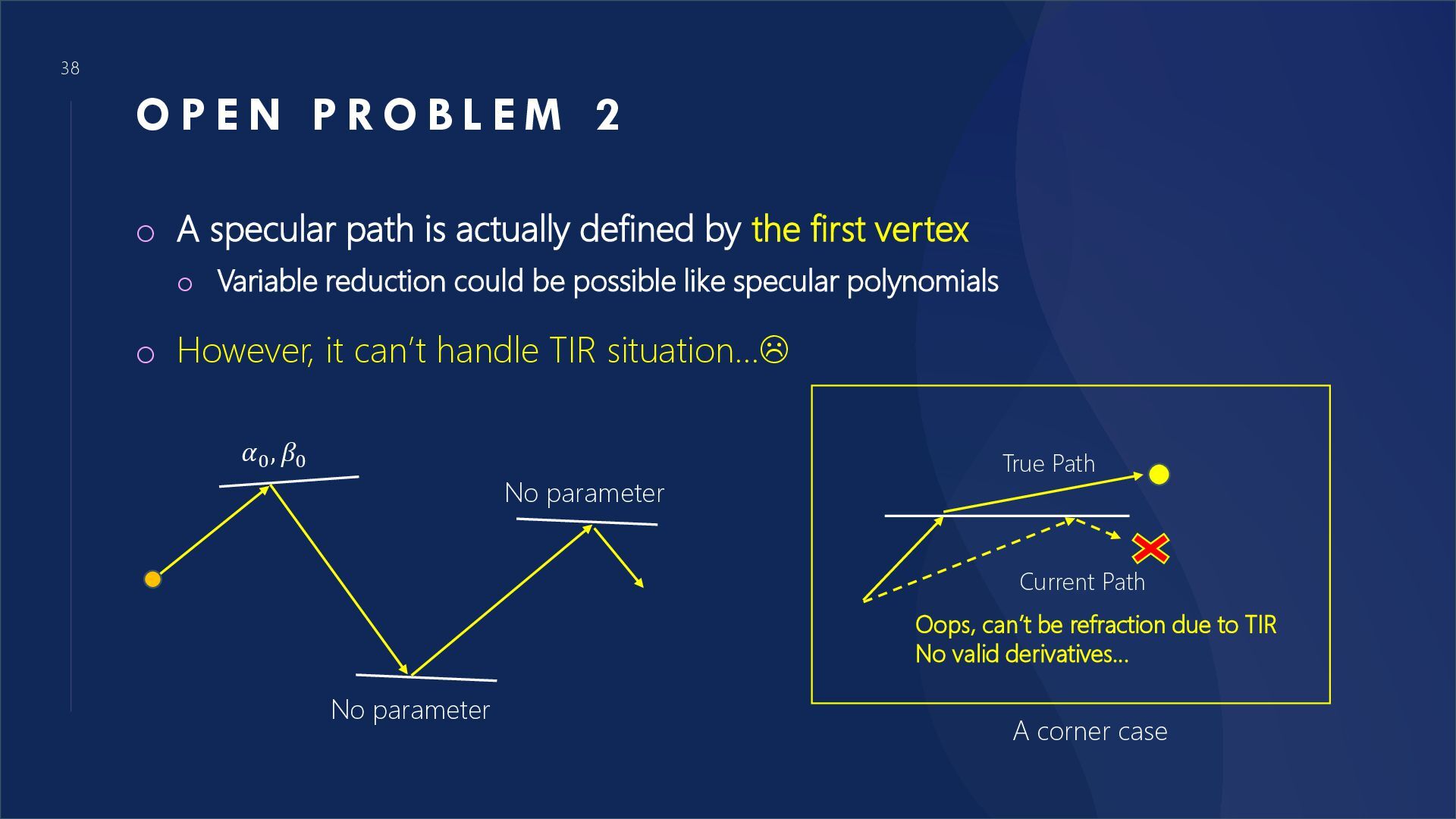
M 2 o A specular path is actually defined by the first vertex o Variable reduction could be possible like specular polynomials o However, it can’t handle TIR situation… 𝛼0 , 𝛽0 No parameter No parameter True Path Current Path Oops, can’t be refraction due to TIR No valid derivatives… A corner case
![10 [ S TA G E 1 ] F I](https://files.speakerdeck.com/presentations/dcb71dd71f7f4935ab98d74f42fe3559/slide_9.jpg)
![17 [ S TA G E 2 ] RO O](https://files.speakerdeck.com/presentations/dcb71dd71f7f4935ab98d74f42fe3559/slide_16.jpg)