Introduction to Algorithms: Computational Complexity

Transcript

1. INTRODUCTION TO ALGORITHMS: COMPUTATIONAL COMPLEXITY BY VASYL NAKVASIUK, 2013
2. WHAT IS AN ALGORITHM?
3. WHAT IS AN ALGORITHM? Important issues: correctness, elegance and efficiency. An algorithm is a procedure that takes any of the possible input instances and transforms it to the desired output.
4. EFFICIENCY Is this really necessary?
5. CRITERIA OF EFFICIENCY: Time complexity Space complexity Time complexity ≠ Space complexity ≠ Complexity of algorithm
6. HOW CAN WE MEASURE COMPLEXITY?
7. HOW CAN WE MEASURE COMPLEXITY? EMPIRICAL ANALYSIS (BENCHMARKS) THEORETICAL ANALYSIS (ASYMPTOTIC ANALYSIS)
8. BENCHMARKS EMPIRICAL ANALYSIS
9. BENCHMARKS VERSION #1 WHAT MEANS “FAST”?
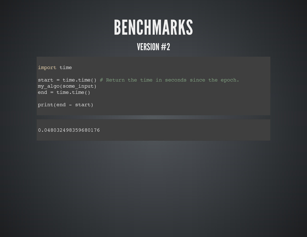
10. BENCHMARKS VERSION #2 i m p o r t t i m e s t a r t = t i m e . t i m e ( ) # R e t u r n t h e t i m e i n s e c o n d s s i n c e t h e e p o c h . m y _ a l g o ( s o m e _ i n p u t ) e n d = t i m e . t i m e ( ) p r i n t ( e n d - s t a r t ) 0 . 0 4 8 0 3 2 4 9 8 3 5 9 6 8 0 1 7 6
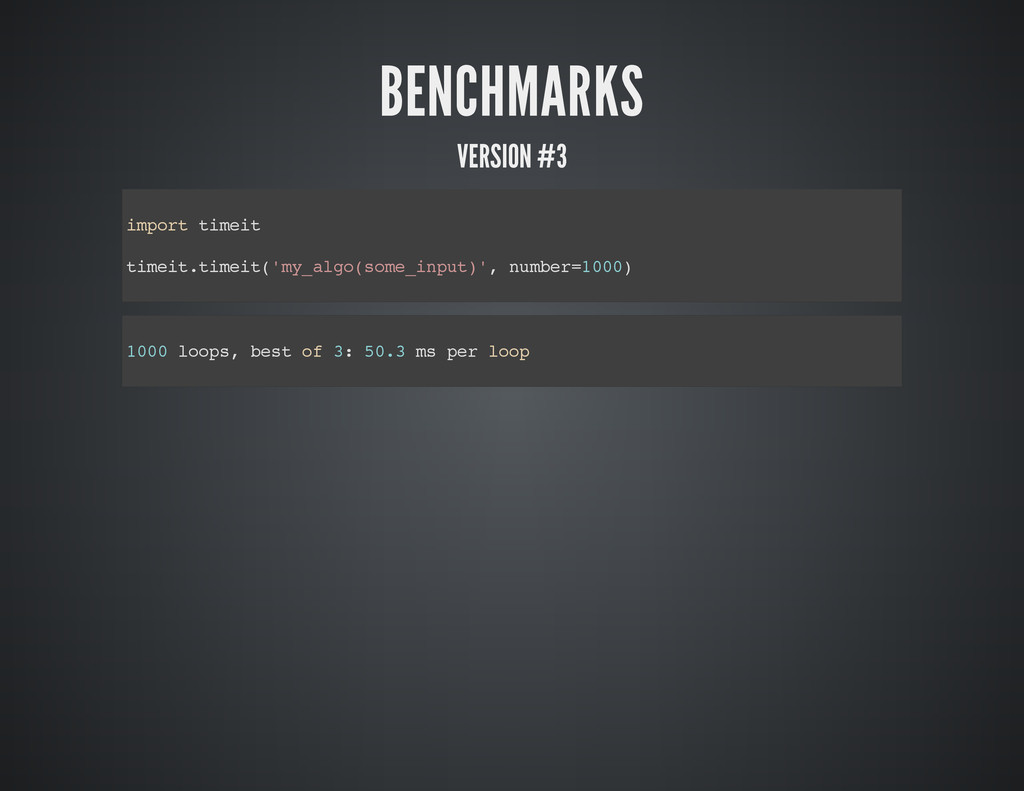
11. BENCHMARKS VERSION #3 i m p o r t t i m e i t t i m e i t . t i m e i t ( ' m y _ a l g o ( s o m e _ i n p u t ) ' , n u m b e r = 1 0 0 0 ) 1 0 0 0 l o o p s , b e s t o f 3 : 5 0 . 3 m s p e r l o o p
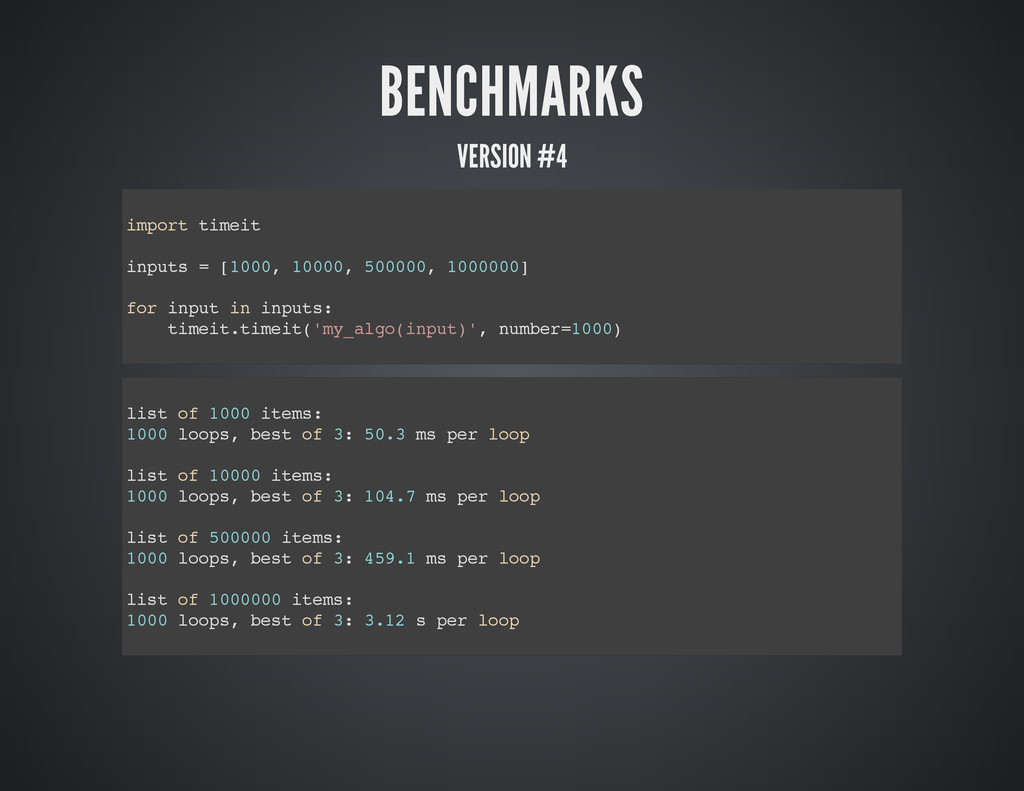
12. BENCHMARKS VERSION #4 i m p o r t t i m e i t i n p u t s = [ 1 0 0 0 , 1 0 0 0 0 , 5 0 0 0 0 0 , 1 0 0 0 0 0 0 ] f o r i n p u t i n i n p u t s : t i m e i t . t i m e i t ( ' m y _ a l g o ( i n p u t ) ' , n u m b e r = 1 0 0 0 ) l i s t o f 1 0 0 0 i t e m s : 1 0 0 0 l o o p s , b e s t o f 3 : 5 0 . 3 m s p e r l o o p l i s t o f 1 0 0 0 0 i t e m s : 1 0 0 0 l o o p s , b e s t o f 3 : 1 0 4 . 7 m s p e r l o o p l i s t o f 5 0 0 0 0 0 i t e m s : 1 0 0 0 l o o p s , b e s t o f 3 : 4 5 9 . 1 m s p e r l o o p l i s t o f 1 0 0 0 0 0 0 i t e m s : 1 0 0 0 l o o p s , b e s t o f 3 : 3 . 1 2 s p e r l o o p
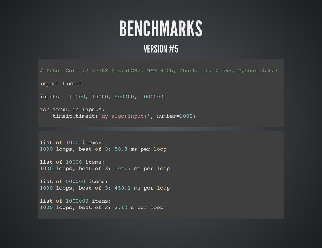
13. BENCHMARKS VERSION #5 # I n t e l C o r e i 7 - 3 9 7 0 X @ 3 . 5 0 G H z , R A M 8 G b , U b u n t u 1 2 . 1 0 x 6 4 , P y t h o n 3 . 3 . 0 i m p o r t t i m e i t i n p u t s = [ 1 0 0 0 , 1 0 0 0 0 , 5 0 0 0 0 0 , 1 0 0 0 0 0 0 ] f o r i n p u t i n i n p u t s : t i m e i t . t i m e i t ( ' m y _ a l g o ( i n p u t ) ' , n u m b e r = 1 0 0 0 ) l i s t o f 1 0 0 0 i t e m s : 1 0 0 0 l o o p s , b e s t o f 3 : 5 0 . 3 m s p e r l o o p l i s t o f 1 0 0 0 0 i t e m s : 1 0 0 0 l o o p s , b e s t o f 3 : 1 0 4 . 7 m s p e r l o o p l i s t o f 5 0 0 0 0 0 i t e m s : 1 0 0 0 l o o p s , b e s t o f 3 : 4 5 9 . 1 m s p e r l o o p l i s t o f 1 0 0 0 0 0 0 i t e m s : 1 0 0 0 l o o p s , b e s t o f 3 : 3 . 1 2 s p e r l o o p
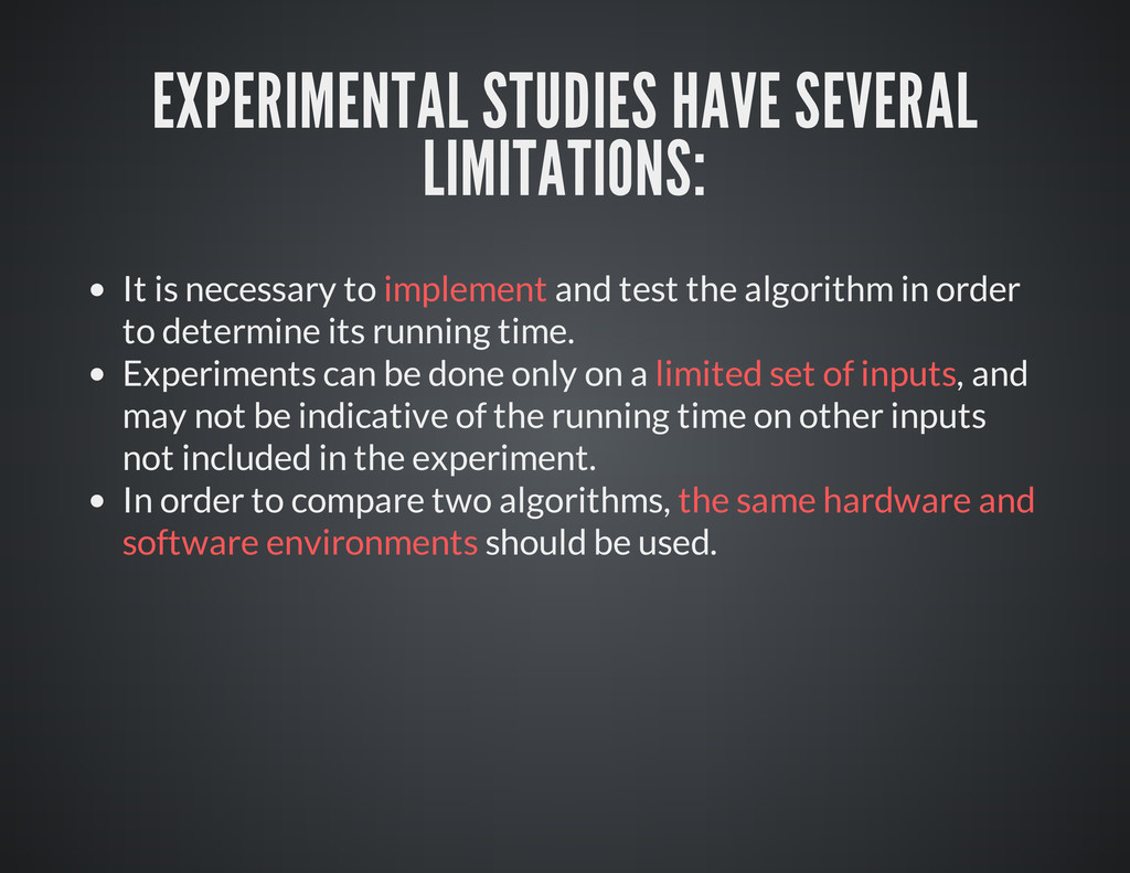
14. EXPERIMENTAL STUDIES HAVE SEVERAL LIMITATIONS: It is necessary to implement and test the algorithm in order to determine its running time. Experiments can be done only on a limited set of inputs, and may not be indicative of the running time on other inputs not included in the experiment. In order to compare two algorithms, the same hardware and software environments should be used.
15. ASYMPTOTIC ANALYSIS THEORETICAL ANALYSIS
16. ASYMPTOTIC ANALYSIS EFFICIENCY AS A FUNCTION OF INPUT SIZE T(n) – running time as a function of n, where n – size of input. n → ∞ Random-Access Machine (RAM)
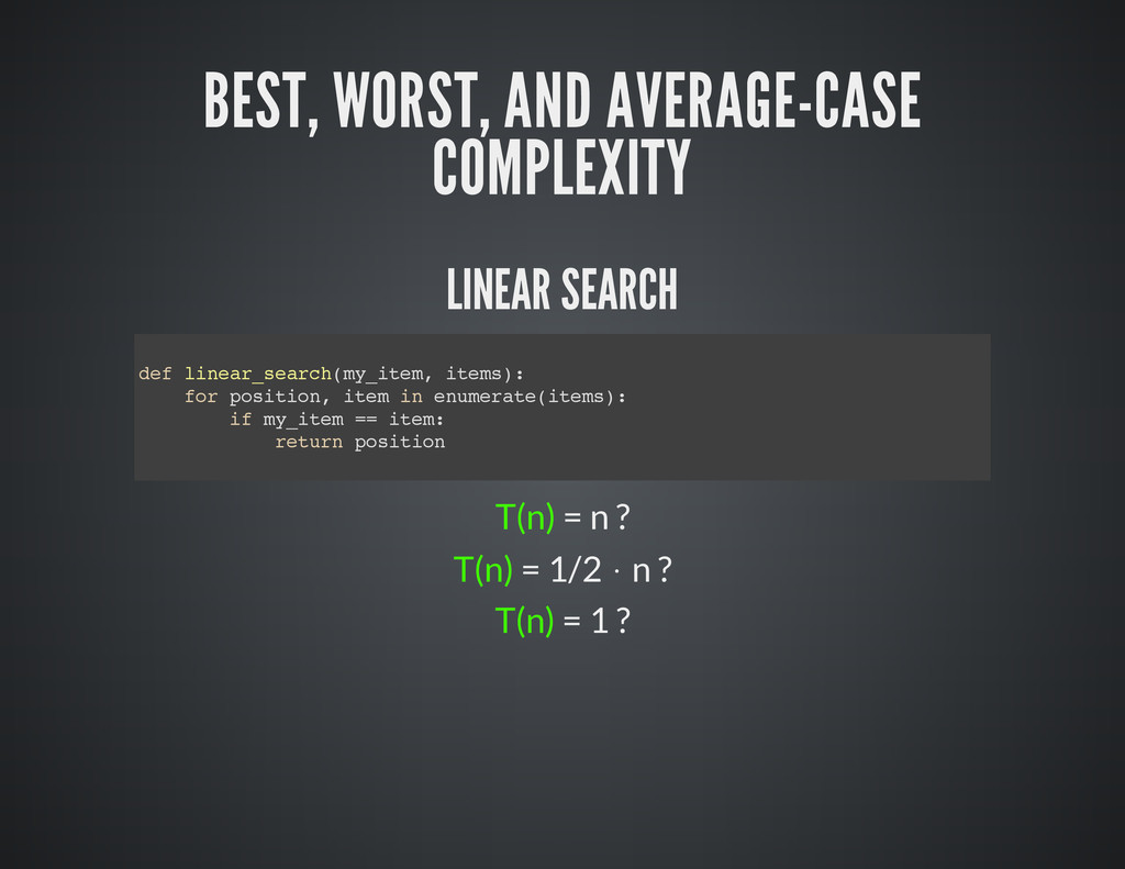
17. BEST, WORST, AND AVERAGE-CASE COMPLEXITY LINEAR SEARCH T(n) = n ? T(n) = 1/2 ⋅ n ? T(n) = 1 ? d e f l i n e a r _ s e a r c h ( m y _ i t e m , i t e m s ) : f o r p o s i t i o n , i t e m i n e n u m e r a t e ( i t e m s ) : i f m y _ i t e m = = i t e m : r e t u r n p o s i t i o n
18. BEST, WORST, AND AVERAGE-CASE COMPLEXITY
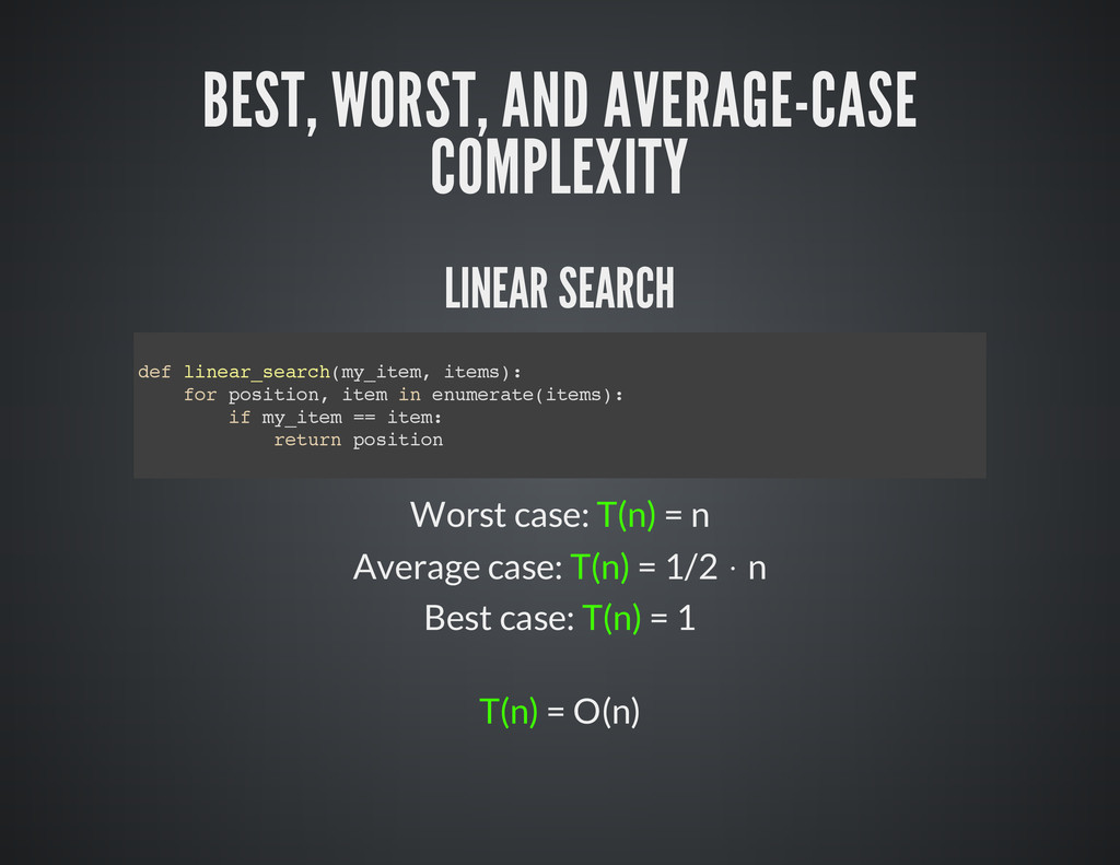
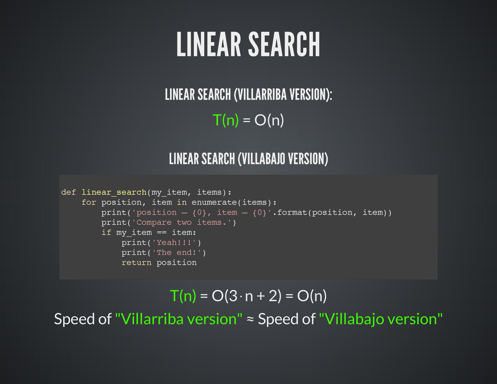
19. BEST, WORST, AND AVERAGE-CASE COMPLEXITY LINEAR SEARCH Worst case: T(n) = n Average case: T(n) = 1/2 ⋅ n Best case: T(n) = 1 T(n) = O(n) d e f l i n e a r _ s e a r c h ( m y _ i t e m , i t e m s ) : f o r p o s i t i o n , i t e m i n e n u m e r a t e ( i t e m s ) : i f m y _ i t e m = = i t e m : r e t u r n p o s i t i o n
20. HOW CAN WE COMPARE TWO FUNCTIONS? WE CAN USE ASYMPTOTIC NOTATION
21. ASYMPTOTIC NOTATION
22. THE BIG OH NOTATION ASYMPTOTIC UPPER BOUND O(g(n)) = {f(n): there exist positive constants c and n0 such that 0 ≤ f(n) ≤ c⋅g(n) for all n ≥ n0} T(n) ∈ O(g(n)) or T(n) = O(g(n))
23. Ω-NOTATION ASYMPTOTIC LOWER BOUND Ω(g(n)) = {f(n): there exist positive constants c and n0 such that 0 ≤ c⋅g(n) ≤ f(n) for all n ≥ n0} T(n) ∈ Ω(g(n)) or T(n) = Ω(g(n))
24. Θ-NOTATION ASYMPTOTIC TIGHT BOUND Θ(g(n)) = {f(n): there exist positive constants c1, c2 and n0 such that 0 ≤ c1⋅g(n) ≤ f(n) ≤ c2⋅g(n) for all n ≥ n0} T(n) ∈ Θ(g(n)) or T(n) = Θ(g(n))
25. GRAPHIC EXAMPLES OF THE Θ, O AND Ω NOTATIONS
26. EXAMPLES 3⋅n2 - 100⋅n + 6 = O(n2), because we can choose c = 3 and 3⋅n2 > 3⋅n2 - 100⋅n + 6 100⋅n2 - 70⋅n - 1 = O(n2), because we can choose c = 100 and 100⋅n2 > 100⋅n2 - 70⋅n - 1 3⋅n2 - 100⋅n + 6 ≈ 100⋅n2 - 70⋅n - 1
27. LINEAR SEARCH LINEAR SEARCH (VILLARRIBA VERSION): T(n) = O(n) LINEAR SEARCH (VILLABAJO VERSION) T(n) = O(3⋅n + 2) = O(n) Speed of "Villarriba version" ≈ Speed of "Villabajo version" d e f l i n e a r _ s e a r c h ( m y _ i t e m , i t e m s ) : f o r p o s i t i o n , i t e m i n e n u m e r a t e ( i t e m s ) : p r i n t ( ' p o s i t i o n – { 0 } , i t e m – { 0 } ' . f o r m a t ( p o s i t i o n , i t e m ) ) p r i n t ( ' C o m p a r e t w o i t e m s . ' ) i f m y _ i t e m = = i t e m : p r i n t ( ' Y e a h ! ! ! ' ) p r i n t ( ' T h e e n d ! ' ) r e t u r n p o s i t i o n
28. TYPES OF ORDER However, all you really need to understand is that: n! ≫ 2n ≫ n3 ≫ n2 ≫ n⋅log(n) ≫ n ≫ log(n) ≫ 1
29. THE BIG OH COMPLEXITY FOR DIFFERENT FUNCTIONS
30. GROWTH RATES OF COMMON FUNCTIONS MEASURED IN NANOSECONDS Each operation takes one nanosecond (10-9 seconds). CPU ≈ 1 GHz
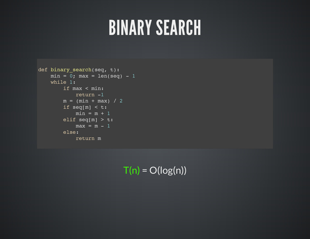
31. BINARY SEARCH T(n) = O(log(n)) d e f b i n a r y _ s e a r c h ( s e q , t ) : m i n = 0 ; m a x = l e n ( s e q ) - 1 w h i l e 1 : i f m a x < m i n : r e t u r n - 1 m = ( m i n + m a x ) / 2 i f s e q [ m ] < t : m i n = m + 1 e l i f s e q [ m ] > t : m a x = m - 1 e l s e : r e t u r n m
32. PRACTICAL USAGE ADD DB “INDEX” Search with index vs Search without index Binary search vs Linear search O(log(n)) vs O(n)
33. HOW CAN YOU QUICKLY FIND OUT COMPLEXITY? O(?)
34. D. E. Knuth, "Big Omicron and Big Omega and BIg Theta", SIGACT News, 1976. On the basis of the issues discussed here, I propose that members of SIGACT, and editors of computer science and mathematics journals, adopt the O, Ω and Θ notations as defined above, unless a better alternative can be found reasonably soon.
35. BENCHMARKS OR ASYMPTOTIC ANALYSIS? USE BOTH APPROACHES!
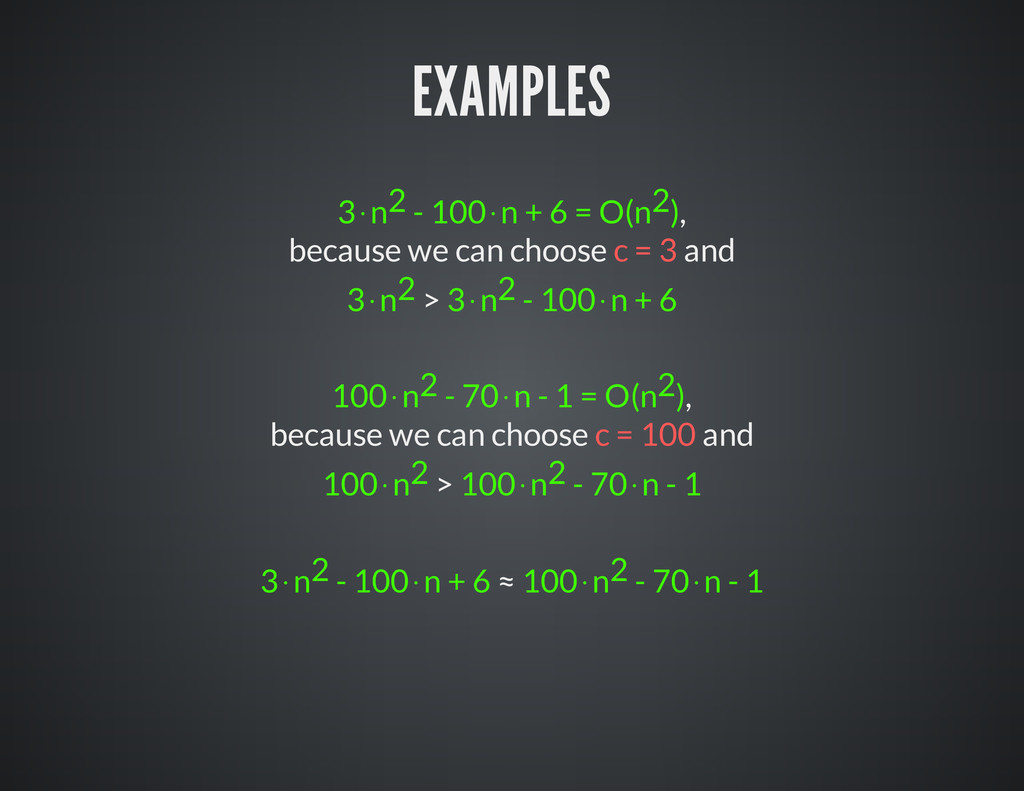
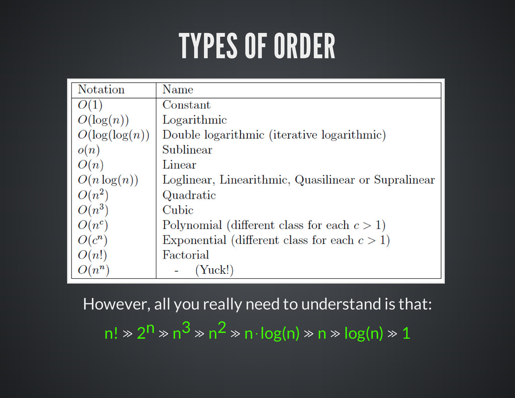
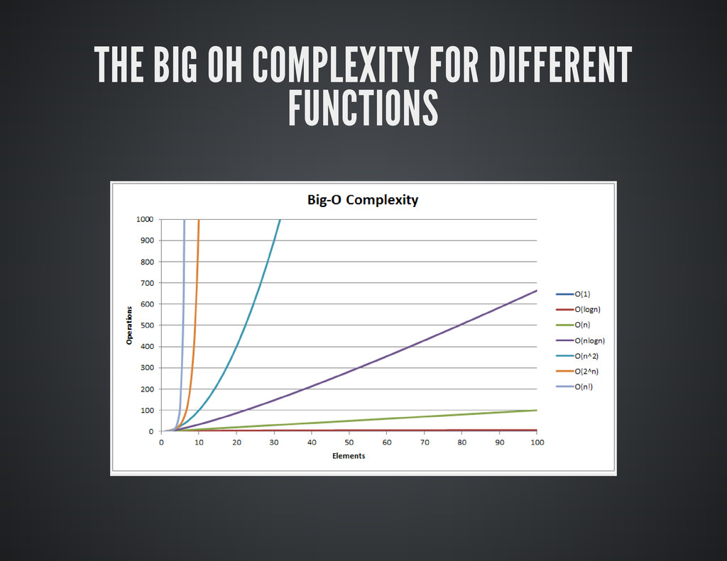
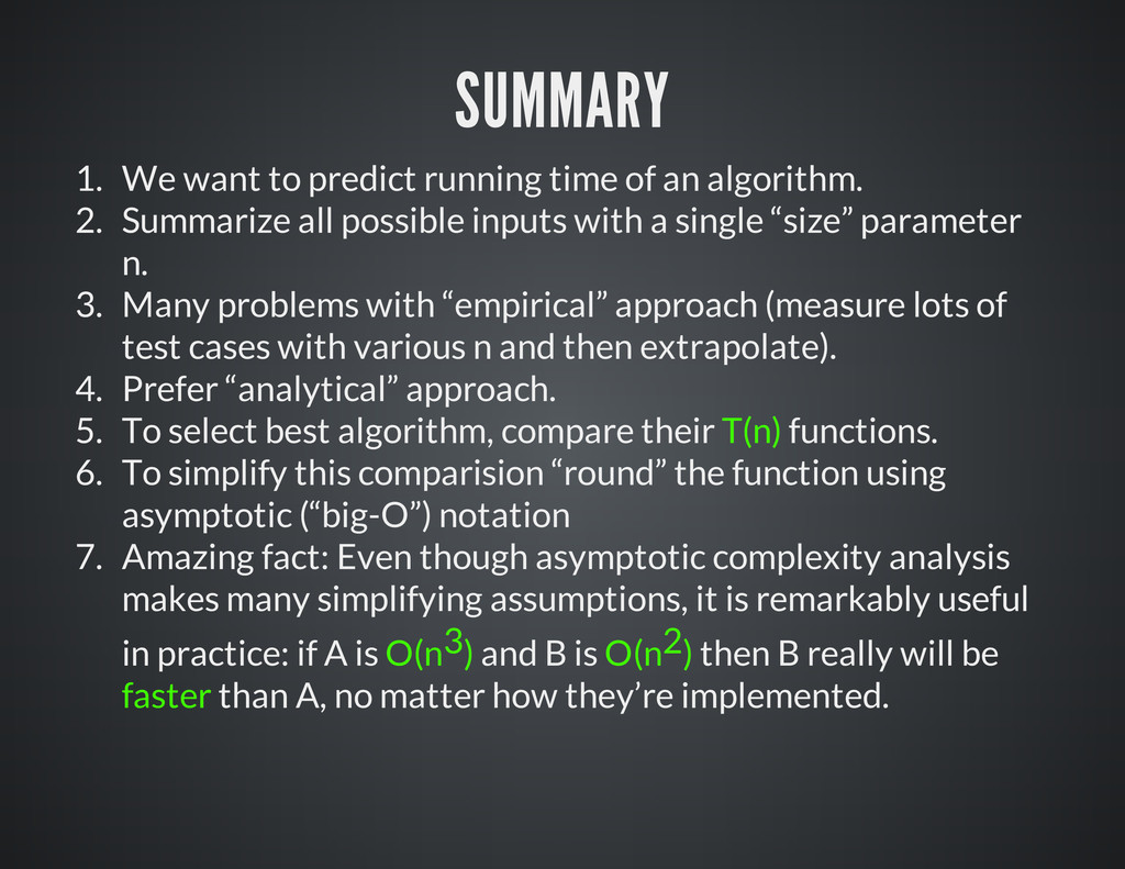
36. SUMMARY 1. We want to predict running time of an algorithm. 2. Summarize all possible inputs with a single “size” parameter n. 3. Many problems with “empirical” approach (measure lots of test cases with various n and then extrapolate). 4. Prefer “analytical” approach. 5. To select best algorithm, compare their T(n) functions. 6. To simplify this comparision “round” the function using asymptotic (“big-O”) notation 7. Amazing fact: Even though asymptotic complexity analysis makes many simplifying assumptions, it is remarkably useful in practice: if A is O(n3) and B is O(n2) then B really will be faster than A, no matter how they’re implemented.
37. LINKS BOOKS: “Introduction To Algorithms, Third Edition”, 2009, by Thomas H. Cormen, Charles E. Leiserson, Ronald L. Rivest and Clifford Stein “The Algorithm Design Manual, Second Edition”, 2008, by Steven S. Skiena OTHER: “Algorithms: Design and Analysis” by Tim Roughgarden Big-O Algorithm Complexity Cheat Sheet https://www.coursera.org/course/algo http://bigocheatsheet.com/
38. THE END THANK YOU FOR ATTENTION! Vasyl Nakvasiuk Email: vaxxxa@gmail.com Twitter: @vaxXxa Github: vaxXxa THIS PRESENTATION: Source: Live: https://github.com/vaxXxa/talks http://vaxXxa.github.io/talks