Introduction to deep learning

Transcript

1. Sensitivity: Internal & Restricted Deep Learning Vidyasagar Bhargava
2. Sensitivity: Internal & Restricted Contents 1. Introduction 2. Why deep learning? 3. Fundamentals of deep learning 4. How deep learning works? 5. Activation Function 6. Train Neural Network • How to minimize loss or cost? • How to move in right direction? • Stochastic Gradient Descent • How to calculate gradient? 7. Adaptive learning 8. Over fitting 9. Regularization 10. H2O • Introduction • H2O’s Deep learning • Features • Parameters • Demo
3. Sensitivity: Internal & Restricted Introduction • Deep learning is an enhanced and powerful form of neural network which is build on several hidden layers(more than 2) • Since Data comes in many forms sometimes its difficult for linear methods to detect non-linearity in the data. In fact, many a times even non-linear algorithm such as GBM, decision tree fails to learn from data. • In such cases, a multi layered neural network which creates non- linear interaction among the features gives the better solution!
4. Sensitivity: Internal & Restricted Why Deep Learning? • Neural Network has been around quite long time and only in past few years they become so popular. • Deep learning is powerful because it is able to learn powerful feature representation in unsupervised manner which differs from traditional machine learning algorithm where we have to manually handcraft features. • Handcraft features works in a lot of domain but some domains like image classification where data is very high dimensional and makes it difficult to craft feature that are useful for prediction. • So deep learning takes the approach to take all the data and figuring out what are the best features.
5. Sensitivity: Internal & Restricted A Perceptron
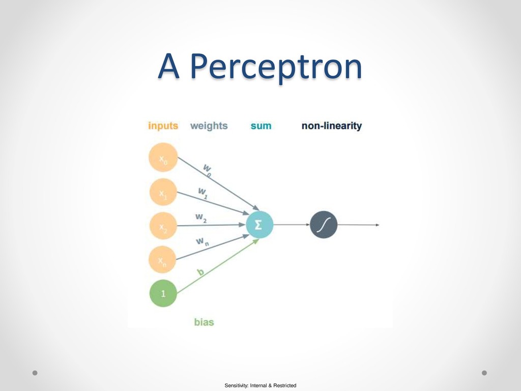
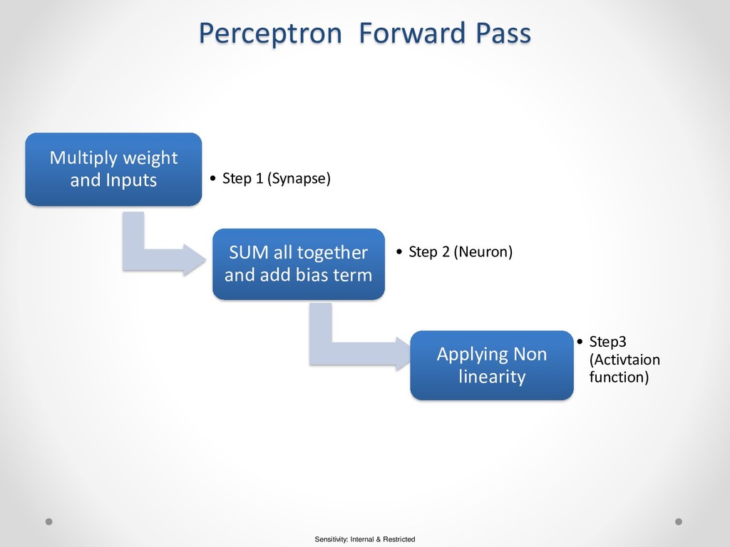
6. Sensitivity: Internal & Restricted Fundamentals of Deep learning • At the core of any neural network is a perceptron • In neural network visual… circle represents neuron and line represents synapse. • Synapse has very simple job they take value from neuron and multiply by specific weight and output the result. • Neurons are little bit complicated.. their job is to add together the outputs from all the synapses add a bias term and apply the activation function. • Activation function allow neural net to model complex non linear pattern.
7. Sensitivity: Internal & Restricted Perceptron Forward Pass Multiply weight and Inputs • Step 1 (Synapse) SUM all together and add bias term • Step 2 (Neuron) Applying Non linearity • Step3 (Activtaion function)
8. Sensitivity: Internal & Restricted Why is bias added ? • Bias is similar to the intercept term in linear regression. • It helps in achieving better prediction by shifting the decision boundary
9. Sensitivity: Internal & Restricted Activation function • At the core of every activation function is non linearity which transforms output from linear feature to non linear feature. • There are many -many activation functions . • Some common activation functions are :- Sigmoid, TanH, ReLu,
10. Sensitivity: Internal & Restricted Importance of Activation function • Activation functions add non linearity to our network’s function. • Non linearity is important because most of our real world data is non linear.
11. Sensitivity: Internal & Restricted How to build neural network with perceptron? • Perceptron is very basic of neural network. However, perceptron isn’t powerful enough to work on linearly separable data. • Due to this Multi-Layer Perceptron came into existence • We can add a hidden layer between input layer and output layer which gives rise to Multi-Layer Perceptron. (MLP) • To extend MLP to deep neural network simply add more layers.
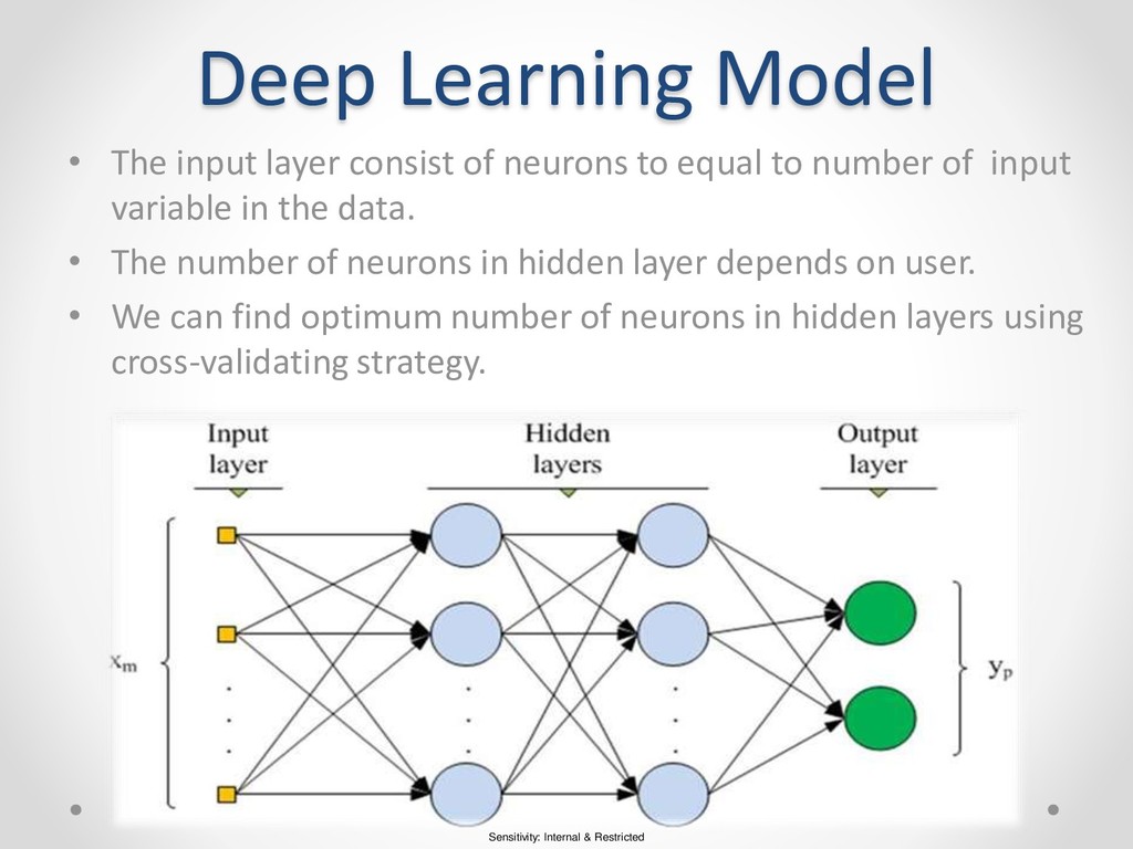
12. Sensitivity: Internal & Restricted Deep Learning Model • The input layer consist of neurons to equal to number of input variable in the data. • The number of neurons in hidden layer depends on user. • We can find optimum number of neurons in hidden layers using cross-validating strategy.
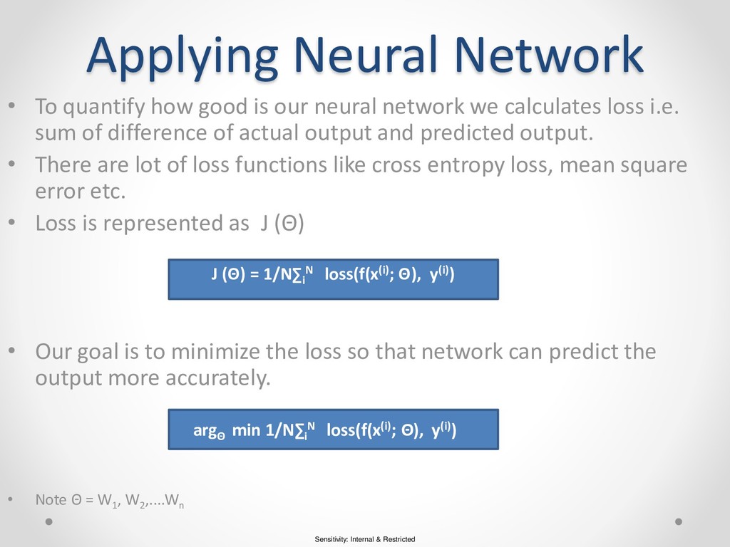
13. Sensitivity: Internal & Restricted Applying Neural Network • To quantify how good is our neural network we calculates loss i.e. sum of difference of actual output and predicted output. • There are lot of loss functions like cross entropy loss, mean square error etc. • Loss is represented as J (Θ) • Our goal is to minimize the loss so that network can predict the output more accurately. • Note Θ = W1 , W2 ,....Wn J (Θ) = 1/N∑i N loss(f(x(i); Θ), y(i)) argΘ min 1/N∑i N loss(f(x(i); Θ), y(i))
14. Sensitivity: Internal & Restricted Train Neural Network • Now we have J (Θ) we express out loss and we will train our neural network to minimize the loss. • So the objective is find the theta that minimizes the loss function. • Theta is just weights of our network. • So loss is a function of the model’s parameters. • To minimize the loss we need to find the lowest point.
15. Sensitivity: Internal & Restricted How to minimize loss or cost? • Once the predicted value is computed, it propagates back layer by layer and recalculates weights associated with each neuron. • This is known as back propagation. • The back propagation algorithm optimizes the network performance using cost function. • This cost function is minimized using an iterative sequence of steps called the gradient descent algorithm.
16. Sensitivity: Internal & Restricted Gradient Descent: How to move in right direction? • Start at random point and to get to the bottom. • To reach bottom we calculate the gradient at this point which points in the direction of maximum ascent…but we want to go downhill so just multiply by negative 1 and move in opposite direction downward and we form new point based on that. • This way we update our parameters to form new loss. • We can do this over and over again untill we reach the minimum loss(untill we reach convergence)
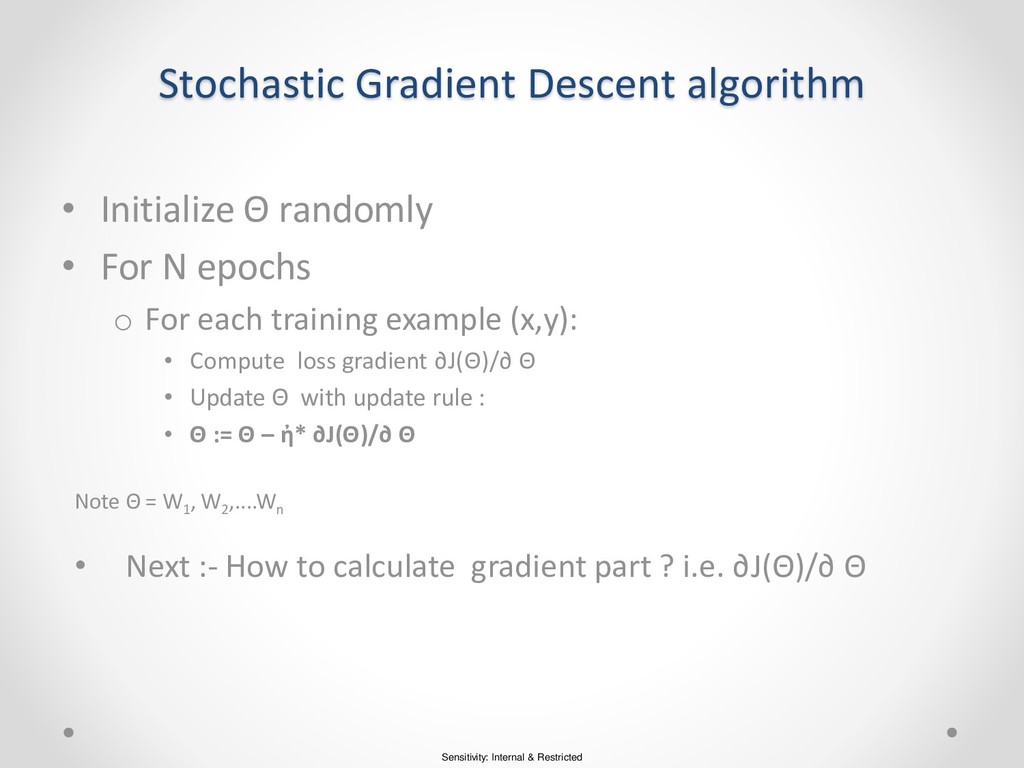
17. Sensitivity: Internal & Restricted Stochastic Gradient Descent algorithm • Initialize Θ randomly • For N epochs o For each training example (x,y): • Compute loss gradient ∂J(Θ)/∂ Θ • Update Θ with update rule : • Θ := Θ – ἠ* ∂J(Θ)/∂ Θ Note Θ = W1 , W2 ,....Wn • Next :- How to calculate gradient part ? i.e. ∂J(Θ)/∂ Θ
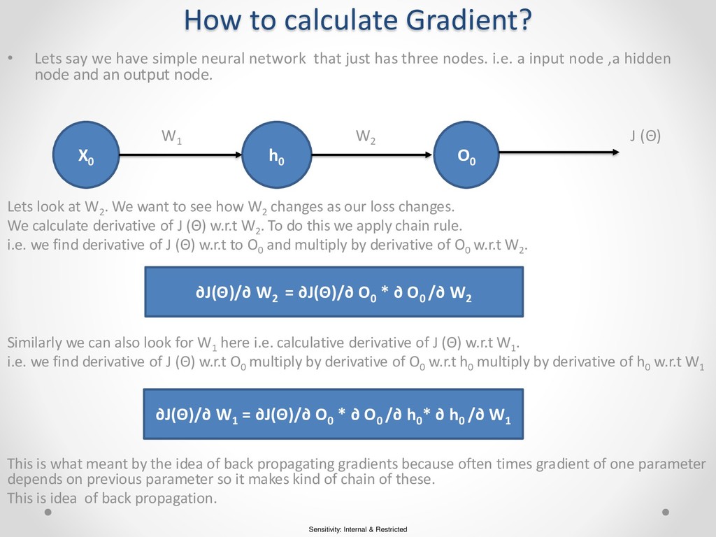
18. Sensitivity: Internal & Restricted How to calculate Gradient? • Lets say we have simple neural network that just has three nodes. i.e. a input node ,a hidden node and an output node. W1 W2 J (Θ) Lets look at W2 . We want to see how W2 changes as our loss changes. We calculate derivative of J (Θ) w.r.t W2 . To do this we apply chain rule. i.e. we find derivative of J (Θ) w.r.t to O0 and multiply by derivative of O0 w.r.t W2 . Similarly we can also look for W1 here i.e. calculative derivative of J (Θ) w.r.t W1 . i.e. we find derivative of J (Θ) w.r.t O0 multiply by derivative of O0 w.r.t h0 multiply by derivative of h0 w.r.t W1 This is what meant by the idea of back propagating gradients because often times gradient of one parameter depends on previous parameter so it makes kind of chain of these. This is idea of back propagation. X0 h0 O0 ∂J(Θ)/∂ W2 = ∂J(Θ)/∂ O0 * ∂ O0 /∂ W2 ∂J(Θ)/∂ W1 = ∂J(Θ)/∂ O0 * ∂ O0 /∂ h0 * ∂ h0 /∂ W1
19. Sensitivity: Internal & Restricted Recap Now we have good idea of :- • 1. How to calculate the gradient? • 2.How to move in the right direction? • 3.How to minimize our loss?
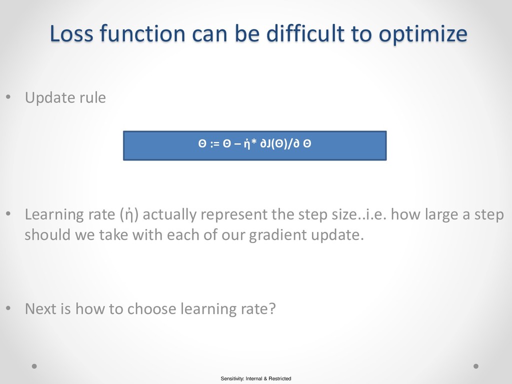
20. Sensitivity: Internal & Restricted Loss function can be difficult to optimize • Update rule • Learning rate (ἠ) actually represent the step size..i.e. how large a step should we take with each of our gradient update. • Next is how to choose learning rate? Θ := Θ – ἠ* ∂J(Θ)/∂ Θ
21. Sensitivity: Internal & Restricted How to choose learning rate (ἠ)? • Small learning rate take lot of time to reach minimum and may be struck in local minima rather global minima • Large learning rate can leads to divergence or increase the loss. • We need to find goldilocks in middle. • There are couple ways like:- guessing…try whole bunch of different values and see what gives best result.its very time consuming and not best use of our resources. • Do something smarter : Adaptive learning rate which adapt and change how learning is going. • We can adapt and change learning rate based on :- o How fast is learning happening? o How large are gradients are? o How large are weights are? o We can have different learning rate for different parameters.
22. Sensitivity: Internal & Restricted Adaptive learning Rate Algorithms • ADAM • Momentum • NAG • Adagrad • Adadelta (H20) • RMSProp For More info on this please check below URL • http://ruder.io/optimizing-gradient-descent/
23. Sensitivity: Internal & Restricted Over fitting • Neural Networks are really powerful models and that are capable of learning all sorts of features and functions. • Sometimes they can be too powerful…i.e. they can either over fit or memorize training examples. • The idea of over fitting is model performs very well on training set but when it comes to real world examples model learnt so specific to training set that it does not apply outside or to test set.
24. Sensitivity: Internal & Restricted Regularization • Regularization is how we prevent over fitting in machine learning or neural networks • Regularization techniques :- • Dropout • Early stop • Weight Regularization • …Others
25. Sensitivity: Internal & Restricted Intro to H2O • H2O is fast, scalable, open-source machine learning and deep learning for smarter application. • Using in-memory compression, H2O handles billions of data rows in-memory, even with a small cluster. • H2O includes many common machine learning algorithms, such as generalized linear modeling (linear regression, logistic regression, etc.), Naive Bayes, principal components analysis, time series, k-means clustering, and others.
26. Sensitivity: Internal & Restricted H2O’s Deep Learning • H2O ‘s Deep Learning is based on multi-layer feed forward artificial neural network that is trained with stochastic gradient descent using back propagation. • A feed forward artificial neural network (ANN) also known as deep neural network(DNN) or multi-layer perceptron(MLP) is the most common type of Deep neural network and the only type that is supported natively in H2O-3. • Other types of DNN such as Convolution Neural Network (CNNs) and Recurrent Neural Network RNN are popular as well. • MLP works well on transactional data (tabular) ,CNN is great choice for particularly image classification and RNN for sequential data (e.g. text, audio, time-series). • H20 deep water project supports CNNs and RNNs through third party integration of deep learning libraries such as Tensorflow, Caffe and MXNet.
27. Sensitivity: Internal & Restricted Features Features of H2O’s deep learning are:- • Multi- threaded distributed parallel computation • Adaptive learning rate for convergence • Regularization options like L1 and L2 • Automatic missing value imputation • Hyper parameter optimization using grid/random search. • For optimization it uses the Hogwild method which is parallelized version of SGD.
28. Sensitivity: Internal & Restricted Parameters • Hidden – It Specifies the number of hidden layer and number of neurons in each layer. • Epochs – It specifies the number of iterations to be done. • Rate –It specifies the learning rate. • Activation-It specifies the type of activation function to use. (In H2O major activation function are TanH, Rectifier and Maxout.)
29. Sensitivity: Internal & Restricted H2O Deep Learning Demo
30. Sensitivity: Internal & Restricted Thank You!