SVM Training in Large Data Sets

Inner seminar of D&Intel Lab.

Transcript

1. SVM TRAINING IN LARGE DATA SETS Weiwei SUN ww.sun@outlook.com
2. Paper Revision • Osuna, E. E., Freund, R., and Girosi, F. (1997b). Support vector machines: Training and applications. Technical report, MIT AI Lab. CBCL. 21 July 2014 Welcome to Southeast University 2
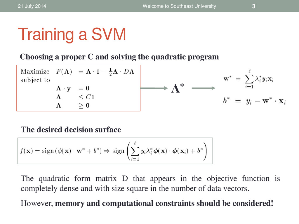
3. Training a SVM 21 July 2014 Welcome to Southeast University 3 Choosing a proper C and solving the quadratic program The desired decision surface Λ* The quadratic form matrix D that appears in the objective function is completely dense and with size square in the number of data vectors. However, memory and computational constraints should be considered!
4. Approach to Large Dataset Training Motivation: Training a SVM using large data sets (above 5000 samples) is a very difficult problem to approach. The matrix D will has 2.5*10^9 entries, and 20GB of memory. Solution: We can solve iteratively the system. Only consider the support vectors, and therefore only optimizing over a reduced set of variables. Then we need to talk about: 1.Optimality conditions: these conditions allow us to decide computationally. 2.Strategy for Improvement: this strategy defines a way to improve the cost function and is frequently associated with variables that violate optimality conditions. 21 July 2014 Welcome to Southeast University 4
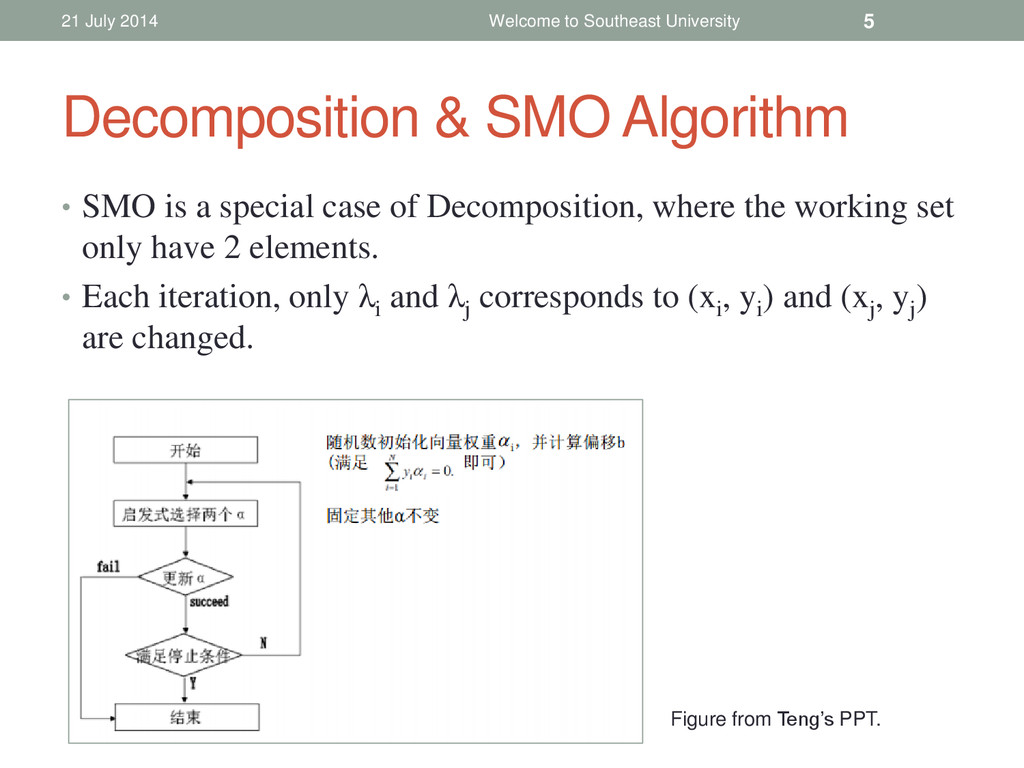
5. Decomposition & SMO Algorithm • SMO is a special case of Decomposition, where the working set only have 2 elements. • Each iteration, only λi and λj corresponds to (xi , yi ) and (xj , yj ) are changed. 21 July 2014 Welcome to Southeast University 5 Figure from Teng’s PPT.
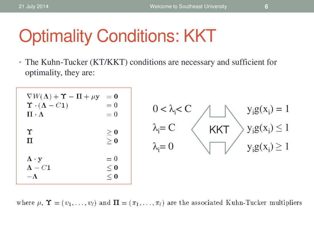
6. Optimality Conditions: KKT • The Kuhn-Tucker (KT/KKT) conditions are necessary and sufficient for optimality, they are: 21 July 2014 Welcome to Southeast University 6 0 < λi < C yi g(xi ) = 1 λi = C yi g(xi ) ≤ 1 λi = 0 yi g(xi ) ≥ 1 KKT
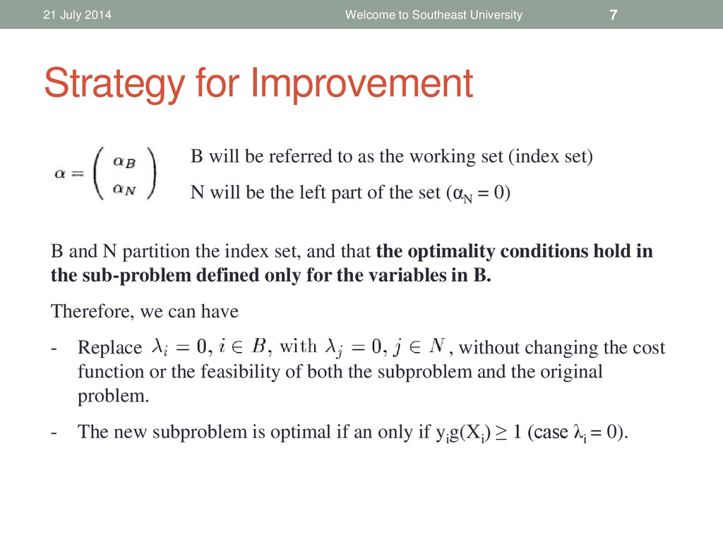
7. Strategy for Improvement 21 July 2014 Welcome to Southeast University 7 B will be referred to as the working set (index set) N will be the left part of the set (αN = 0) B and N partition the index set, and that the optimality conditions hold in the sub-problem defined only for the variables in B. Therefore, we can have - Replace , without changing the cost function or the feasibility of both the subproblem and the original problem. - The new subproblem is optimal if an only if yi g(Xi ) ≥ 1 (case λi = 0).
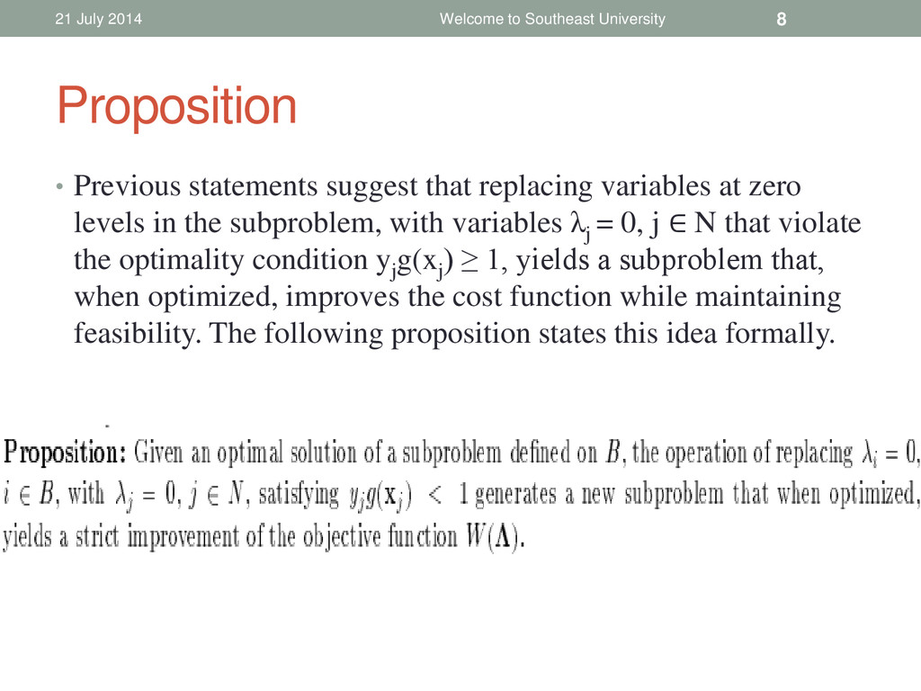
8. Proposition • Previous statements suggest that replacing variables at zero levels in the subproblem, with variables λj = 0, j ∈ N that violate the optimality condition yj g(xj ) ≥ 1, yields a subproblem that, when optimized, improves the cost function while maintaining feasibility. The following proposition states this idea formally. 21 July 2014 Welcome to Southeast University 8
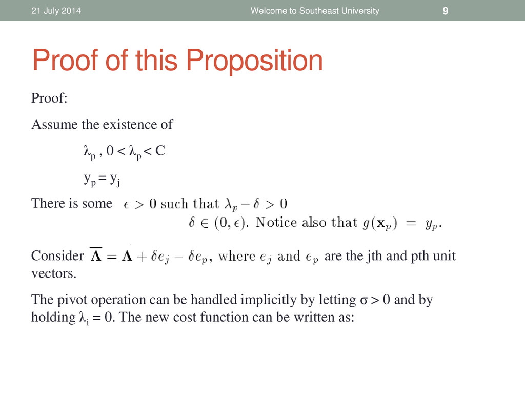
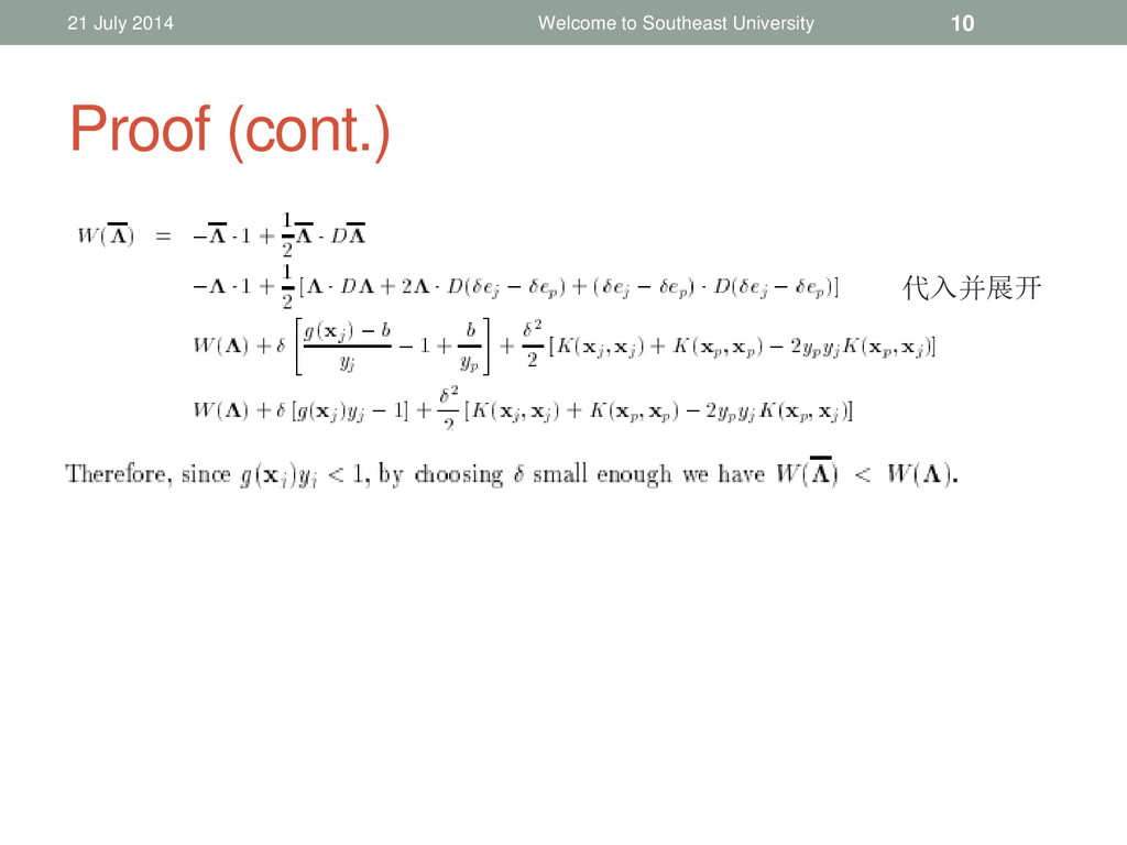
9. Proof of this Proposition 21 July 2014 Welcome to Southeast University 9 Proof: Assume the existence of λp , 0 < λp < C yp = yj There is some Consider are the jth and pth unit vectors. The pivot operation can be handled implicitly by letting σ > 0 and by holding λi = 0. The new cost function can be written as:
10. Proof (cont.) 21 July 2014 Welcome to Southeast University 10 代入并展开
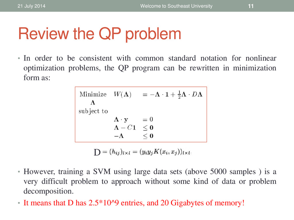
11. Review the QP problem • In order to be consistent with common standard notation for nonlinear optimization problems, the QP program can be rewritten in minimization form as: • However, training a SVM using large data sets (above 5000 samples ) is a very difficult problem to approach without some kind of data or problem decomposition. • It means that D has 2.5*10^9 entries, and 20 Gigabytes of memory! 21 July 2014 Welcome to Southeast University 11 D
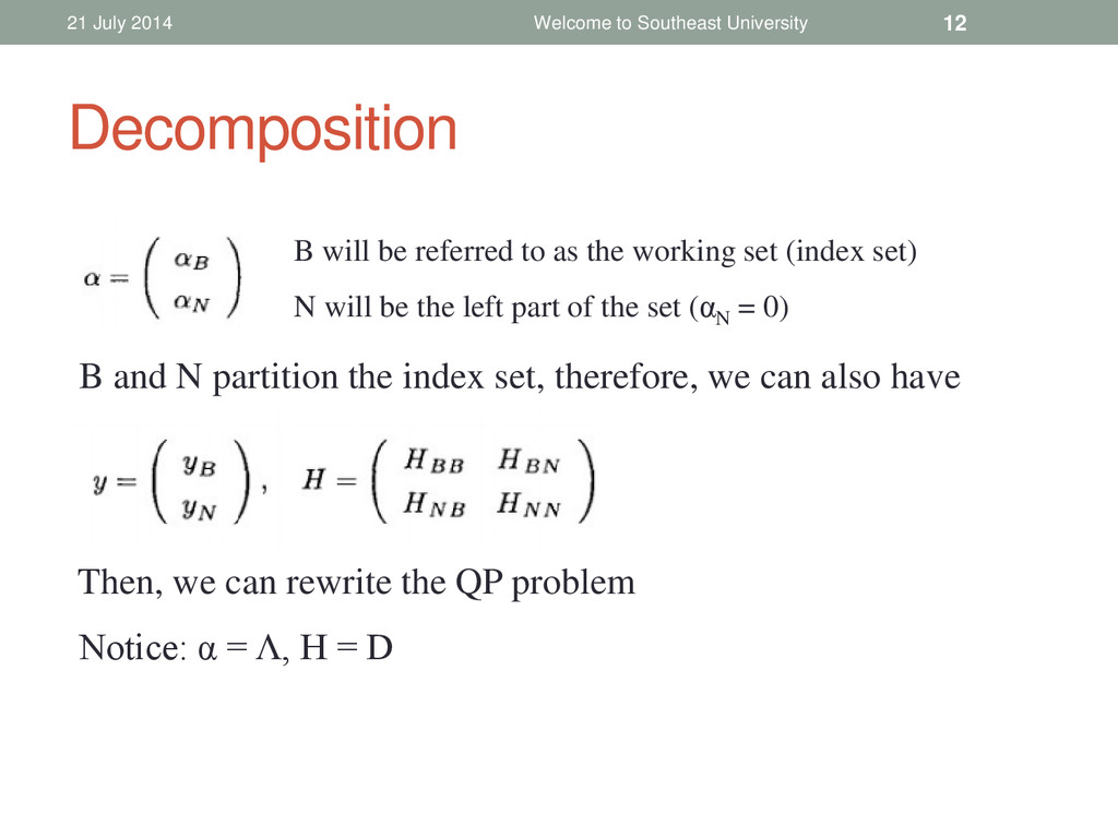
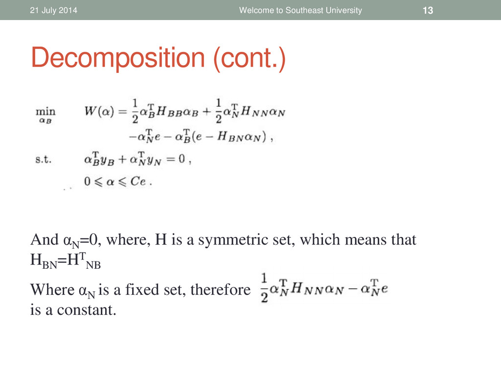
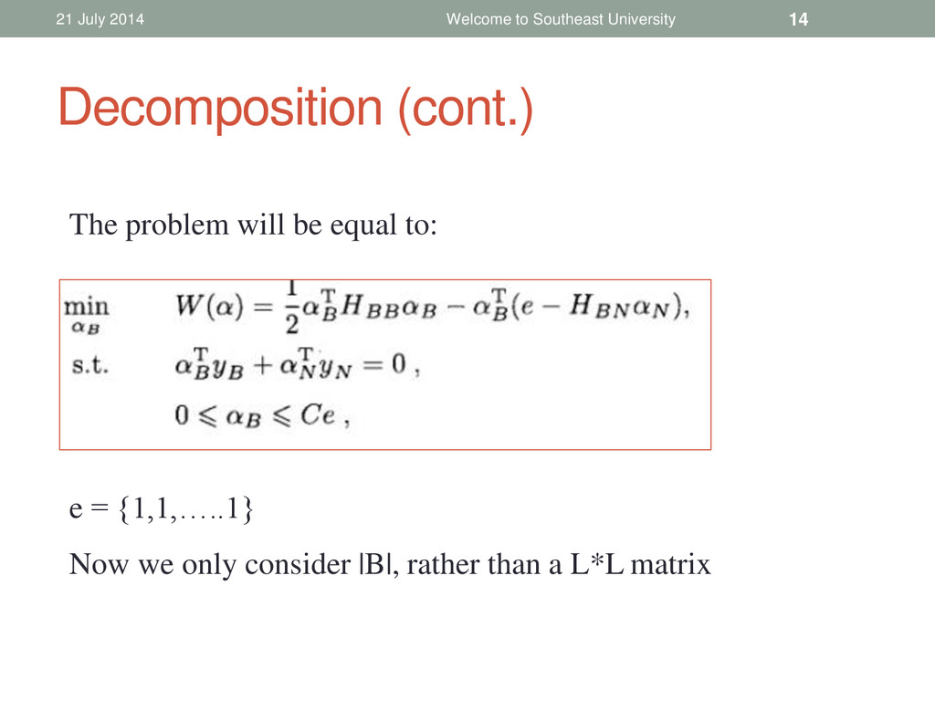
12. Decomposition 21 July 2014 Welcome to Southeast University 12 Notice: α = Λ, H = D B will be referred to as the working set (index set) N will be the left part of the set (αN = 0) B and N partition the index set, therefore, we can also have Then, we can rewrite the QP problem
13. Decomposition (cont.) 21 July 2014 Welcome to Southeast University 13 And αN =0, where, H is a symmetric set, which means that HBN =HT NB Where αN is a fixed set, therefore is a constant.
14. Decomposition (cont.) 21 July 2014 Welcome to Southeast University 14 e = {1,1,…..1} Now we only consider |B|, rather than a L*L matrix The problem will be equal to:
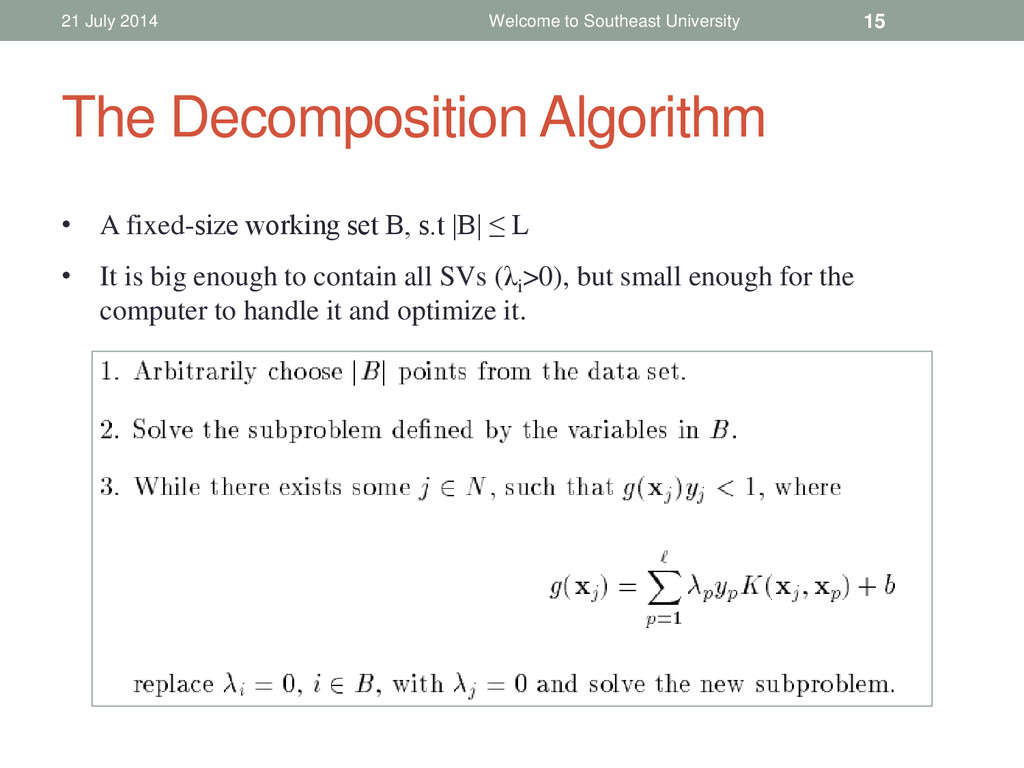
15. The Decomposition Algorithm 21 July 2014 Welcome to Southeast University 15 • A fixed-size working set B, s.t |B| ≤ L • It is big enough to contain all SVs (λi >0), but small enough for the computer to handle it and optimize it.
16. Geometric interpretation 21 July 2014 Welcome to Southeast University 16
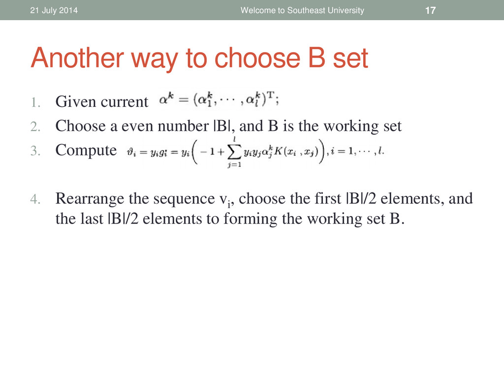
17. Another way to choose B set 1. Given current 2. Choose a even number |B|, and B is the working set 3. Compute 4. Rearrange the sequence vi , choose the first |B|/2 elements, and the last |B|/2 elements to forming the working set B. 21 July 2014 Welcome to Southeast University 17
18. Any questions? 21 July 2014 Welcome to Southeast University 18 Reference: 李航，统计学习方法，2012，清华大学出版社