Reducing the Sampling Complexity of Topic Models

Presented at ACM SIGKDD 2014 in New York. We received KDD 2014 Best Research Paper Award for the underlying research paper.

Transcript

1. Reducing the Sampling Complexity of Topic Models Aaron Li joint work with Amr Ahmed, Sujith Ravi, Alex Smola CMU and Google
2. Outline • Topic Models • Inference algorithms • Losing sparsity at scale • Inference algorithm • Metropolis Hastings proposal • Walker’s Alias method for O(kd) draws • Experiments • LDA, Pitman-Yor topic models, HPYM • Distributed inference
3. Models
4. Clustering & Topic Models Latent Dirichlet Allocation wij zij θi language prior topic probability topic label instance α β ψk
5. Topics in text
 (Blei, Ng, Jordan, 2003)
6. Collapsed Gibbs Sampler
 (Griffiths & Steyvers, 2005) wij zij θi language prior topic probability topic label instance α ψt β n ij(t, d) + ↵t n ij(d) + P t ↵t ⇥ n ij(t, w) + w n ij(t) + P w w
7. • For each document do • For each word in the document do • Resample topic for the word
 
 
 
 
 
 • Update (document, topic) table • Update (word,topic) table Collapsed Gibbs Sampler sparse for small collections sparse for most documents dense n ij(t, d) + ↵t ⇥ n ij(t, w) + w n ij(t) + ¯
8. • For each document do • For each word in the document do • Resample topic for the word
 
 
 
 
 
 • Update (document, topic) table • Update (word,topic) table Exploiting Sparsity
 (Yao, Mimno, Mccallum, 2009) sparse for small collections “constant” ↵t w n ij(t) + ¯ + n ij(t, d) n ij(t, w) + w n ij(t) + ¯ + n ij(t, w) ↵t n ij(t) + ¯ sparse for most documents amortized
 O(kd + kw ) time
9. • For each document do • For each word in the document do • Resample topic for the word
 
 
 
 
 
 • Update (document, topic) table • Update (word,topic) table Exploiting Sparsity
 (Yao, Mimno, Mccallum, 2009) “constant” ↵t w n ij(t) + ¯ + n ij(t, d) n ij(t, w) + w n ij(t) + ¯ + n ij(t, w) ↵t n ij(t) + ¯ sparse for most documents dense for large collections O(k) time we solve this problem
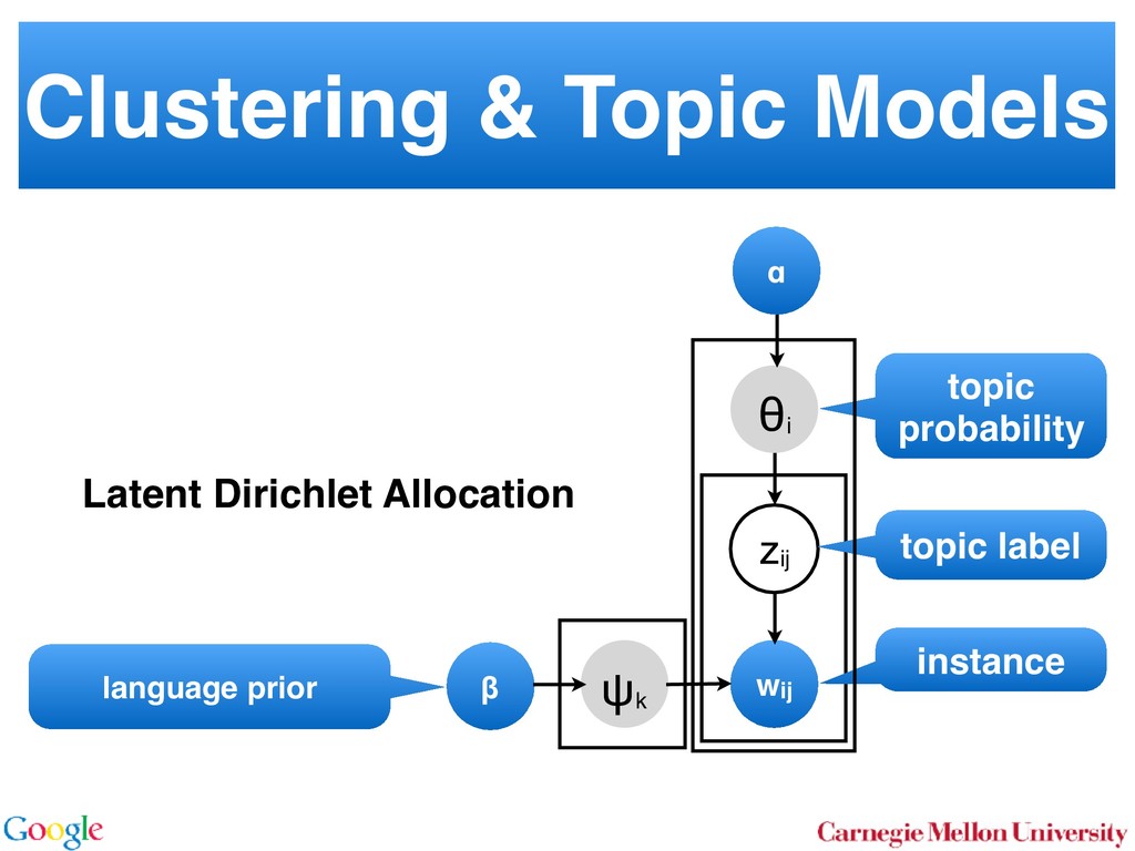
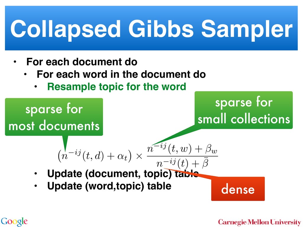
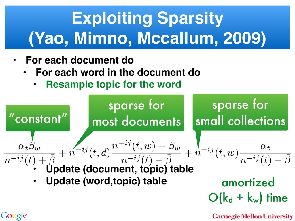
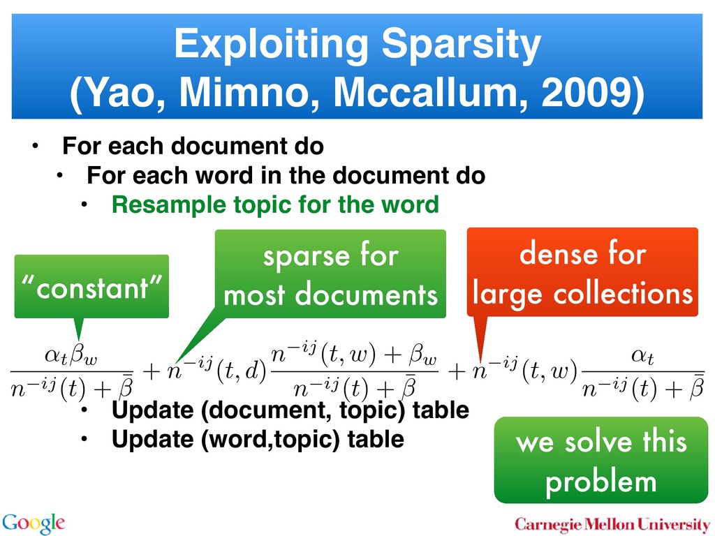
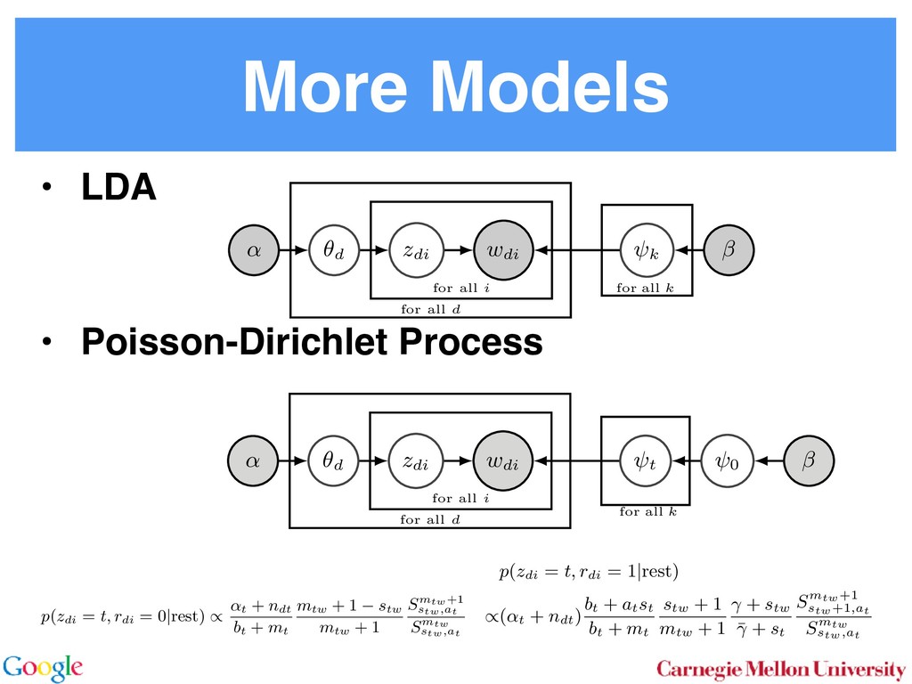
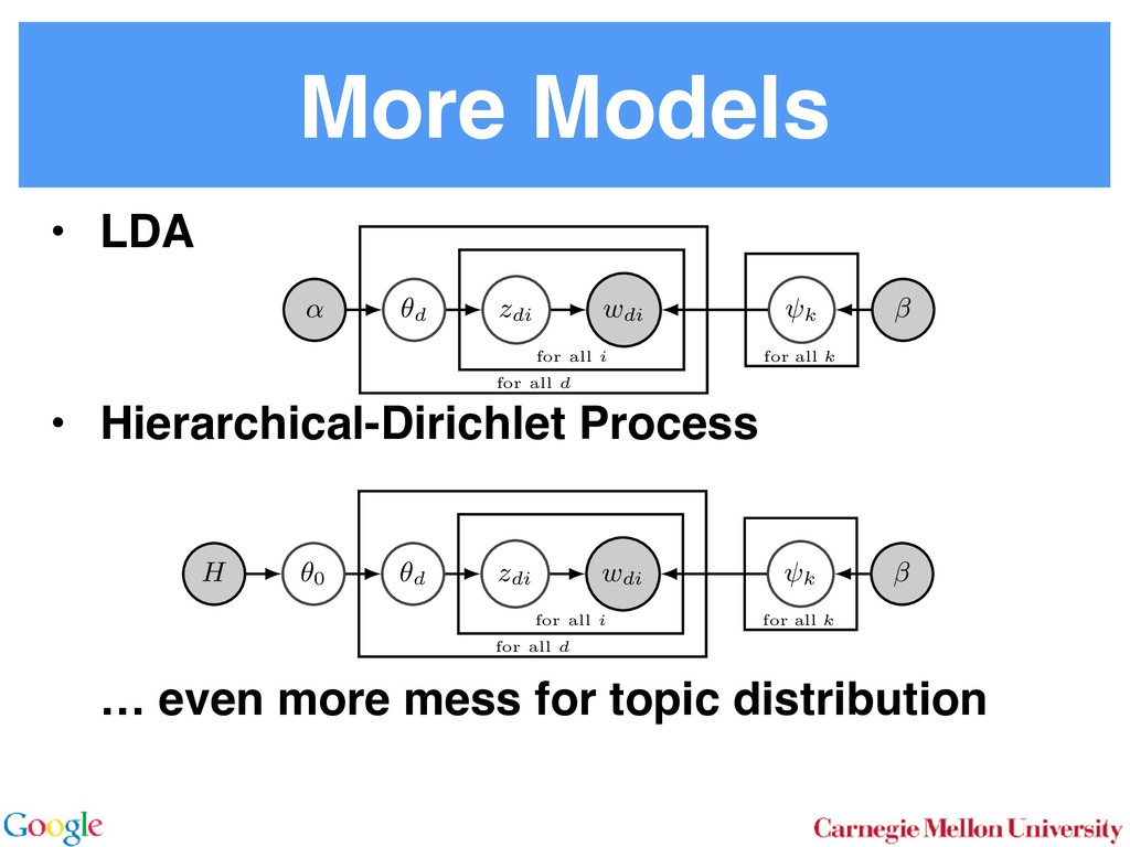
10. More Models • LDA • Poisson-Dirichlet Process 2.1 Latent Dirichlet Allocation In LDA [3] one assumes that documents are mixture dis- tributions of language models associated with individual topics. That is, the documents are generated following the graphical model below: for all i for all d for all k ↵ ✓d zdi wdi k For each document d draw a topic distribution ✓d from a Dirichlet distribution with concentration parameter ↵ ✓d ⇠ Dir(↵). (1) For each topic t draw a word distribution from a Dirichlet distribution with concentration parameter t ⇠ Dir( ). (2) For each word i 2 {1 . . . nd } in document d draw a topic from the multinomial ✓d via Sto sampl using ⌘tw a Unfor carefu dense Inst amort Here in O( numb tional does n gle wo chang the ba 2.2 To with m for all i for all d for all k ↵ ✓d zdi wdi t 0 In a conventional topic model the language model is sim- ply given by a multinomial draw from a Dirichlet distribu- tion. This fails to exploit distribution information between topics, such as the fact that all topics have the same common underlying language. A means for addressing this problem if n Her for rameter a prevents a word to be sampled too often by im- posing a penalty on its probability based on its frequency. The combined model described explicityly in [5]: ✓d ⇠ Dir(↵) 0 ⇠ Dir( ) zdi ⇠ Discrete(✓d ) t ⇠ PDP(b, a, 0 ) wdi ⇠ Discrete ( zdi ) As can be seen, the document-specific part is identical to LDA whereas the language model is rather more sophisti- cated. Likewise, the collapsed inference scheme is analogous to a Chinese Restaurant Process [6, 5]. The technical di - culty arises from the fact that we are dealing with distribu- tions over countable domains. Hence, we need to keep track of multiplicities, i.e. whether any given token is drawn from i or 0 . This will require the introduction of additional count variables in the collapsed inference algorithm. Each topic is equivalent to a restaurant. Each token in the document is equivalent to a customer. Each type of word corresponds each type of dish served by the restaurant. The same results in [6] can be used to derive the conditional probability by introducing axillary variables: • stw denotes the number of tables serving dish w in restaurant t. Here t is the equivalent of a topic. • rdi indicates whether wdi opens a new table in the restaurant or not (to deal with multiplicities). • mtw denotes the number of times dish w has been served in restaurant t (analogously to nwk in LDA). The conditional probability is given by: p(zdi = t, rdi = 0|rest) / ↵t + ndt bt + mt mtw + 1 stw mtw + 1 Smtw+1 stw,at Smtw stw,at (7) over topics. In other words, we add an extra level o chy on the document side (compared to the extra h on the language model used in the PDP). for all i for all d for al H ✓0 ✓d zdi wdi k More formally, the joint distribution is as follows: ✓0 ⇠ DP(b0 , H(·)) t ⇠ Dir( ) ✓d ⇠ DP(b1 , ✓0 ) zdi ⇠ Discrete(✓d ) wdi ⇠ Discrete ( zdi ) By construction, DP(b0 , H(·)) is a Dirichlet Process lent to a Poisson Dirichlet Process PDP(b0 , a, H(·)) discount parameter a set to 0. The base distributio often assumed to be a uniform distribution in most At first, a base ✓0 is drawn from DP(b0 , H(·)). T erns how many topics there are in general, and wh overall prevalence is. The latter is then used in the n of the hierarchy to draw a document-specific distrib that serves the same role as in LDA. The main di↵ that unlike in LDA, we use ✓0 to infer which topics popular than others. It is also possible to extend the model to more t levels of hierarchy, such as the infinite mixture mo Similar to Poisson Dirichlet Process, an equivalent Restaurant Franchise analogy [6, 19] exists for H cal Dirichlet Process with multiple levels. In this each Dirichlet Process is mapped to a single Chinese for all i for all d for all k d zdi wdi t 0 entional topic model the language model is sim- y a multinomial draw from a Dirichlet distribu- if no additional ’table’ is opened by word wdi . Otherwise p(zdi = t, rdi = 1|rest) (8 /(↵t + ndt ) bt + at st bt + mt stw + 1 mtw + 1 + stw ¯ + st Smtw+1 stw+1,at Smtw stw,at Here SN M,a is the generalized Stirling number. It is given b
11. More Models • LDA • Hierarchical-Dirichlet Process
 
 
 
 
 … even more mess for topic distribution 2.1 Latent Dirichlet Allocation In LDA [3] one assumes that documents are mixture dis- tributions of language models associated with individual topics. That is, the documents are generated following the graphical model below: for all i for all d for all k ↵ ✓d zdi wdi k For each document d draw a topic distribution ✓d from a Dirichlet distribution with concentration parameter ↵ ✓d ⇠ Dir(↵). (1) For each topic t draw a word distribution from a Dirichlet distribution with concentration parameter t ⇠ Dir( ). (2) For each word i 2 {1 . . . nd } in document d draw a topic from the multinomial ✓d via Sto sampl using ⌘tw a Unfor carefu dense Inst amort Here in O( numb tional does n gle wo chang the ba 2.2 To with m pus, the portional w from a ility dis- mon un- distribu- del, each base dis- anguage arameter le being ount pa- n by im- equency. 0 ) ntical to sophisti- nalogous cal di - distribu- ep track twice as large space of state variables. 2.3 Hierarchical Dirichlet Process To illustrate the e cacy and generality of our approach we discuss a third case where the document model itself is more sophisticated than a simple collapsed Dirichlet-multinomial. We demonstrate that there, too, inference can be performed e ciently. Consider the two-level topic model based on the Hierarchical Dirichlet Process [19] (HDP-LDA). In it, the topic distribution for each document ✓d is drawn from a Dirichlet process DP(b1 , ✓0 ). In turn, ✓0 is drawn from a Dirichlet process DP(b0 , H(·)) governing the distribution over topics. In other words, we add an extra level of hierar- chy on the document side (compared to the extra hierarchy on the language model used in the PDP). for all i for all d for all k H ✓0 ✓d zdi wdi k More formally, the joint distribution is as follows: ✓0 ⇠ DP(b0 , H(·)) t ⇠ Dir( ) ✓d ⇠ DP(b1 , ✓0 ) zdi ⇠ Discrete(✓d )
12. Key Idea of the Paper • LDA
 
 
 • Approximate slowly changing distribution by fixed distribution. Use Metropolis Hastings • Amortized O(1) time proposals 2.1 Latent Dirichlet Allocation In LDA [3] one assumes that documents are mixture dis- tributions of language models associated with individual topics. That is, the documents are generated following the graphical model below: for all i for all d for all k ↵ ✓d zdi wdi k For each document d draw a topic distribution ✓d from a Dirichlet distribution with concentration parameter ↵ ✓d ⇠ Dir(↵). (1) For each topic t draw a word distribution from a Dirichlet distribution with concentration parameter t ⇠ Dir( ). (2) For each word i 2 {1 . . . nd } in document d draw a topic from the multinomial ✓d via Sto sampl using ⌘tw a Unfor carefu dense Inst amort Here in O( numb tional does n gle wo chang the ba 2.2 To with m slow changes big variation
13. Metropolis Hastings Sampler
14. Lazy decomposition • Exploiting topic sparsity in documents
 
 
 
 
 
 • Normalization costs O(k) operations! n ij(t, d) + ↵t n ij(t, w) + w n ij(t) + P w w =n ij(t, d) n ij(t, w) + w n ij(t) + P w w + ↵t n ij(t, w) + w n ij(t) + P w w Sparse O(kd ) time samples Often dense but slowly varying
15. Lazy decomposition • Exploiting topic sparsity in documents
 
 
 
 
 
 
 • Normalization costs O(kd + 1) operations! n ij(t, d) + ↵t n ij(t, w) + w n ij(t) + P w w =n ij(t, d) n ij(t, w) + w n ij(t) + P w w + ↵t n ij(t, w) + w n ij(t) + P w w Sparse O(kd ) time samples Approximate by stale q(t|w)
16. Lazy decomposition • Exploiting topic sparsity in documents
 
 
 
 
 
 
 • Normalization costs O(kd + 1) operations! Sparse n ij(t, d) + ↵t n ij(t, w) + w n ij(t) + P w w =n ij(t, d) n ij(t, w) + w n ij(t) + P w w + ↵t n ij(t, w) + w n ij(t) + P w w ⇡q(t|d) + q(t|w) Static
17. Metropolis Hastings
 with stationary proposal distribution • We want to sample from p but only have q • Metropolis Hastings • Draw x from q(x) and accept move from x’
 
 • We only need to evaluate ratios of p and q • This is a chain. It mixes rapidly in experiments. min ✓ 1 , p ( x ) p ( x 0) q ( x 0) q ( x ) ◆
18. Application to Topic Models • Recall - we split topic probability • Dense part has normalization precomputed • Sparse part can easily be normalized • Sample from q(t) and 
 evaluate p(t|w,d) only for the draws q(t) / q(t|d) + q(t|w) kd Sparse Dense but static
19. In a nutshell • Sparse part for document
 (topics, topic hierarchy, etc.)
 Evaluate this exactly • Dense part for generative
 model (language, images, …)
 Approximate this by stale model • Metropolis Hastings sampler to correct • Need fast way to draw from stale model q(t) / q(t|d) + q(t|w)
20. Sampling
21. Walker’s Alias Method • Draw from discrete distribution in O(1) time • Requires O(n) preprocessing • Group all x with n p(x) < 1 into L (rest in H) • Fill each of the small ones up by stealing from H. This yields (i,j, p(i)) triples. • Draw from uniform over n, then from p(i)
22. Probability distribution Courtesy of keithschwartz.com
23. Probability distribution Courtesy of keithschwartz.com Splitting
24. Probability distribution Courtesy of keithschwartz.com Filling up (4) with (1)
25. Probability distribution Courtesy of keithschwartz.com Filling up (3) with (1)
26. Probability distribution Courtesy of keithschwartz.com Filling up (1) with (2)
27. Metropolis-Hastings-Walker • Conditional topic probability • Use Walker’s method to draw from q(t|w) • After k draws from q(t|w) recompute with current value • Amortized O(1 + kd) sampler q(t) / q(t|d) + q(t|w) kd Sparse Dense but static
28. Experiments
29. LDA: Varying the number of topics (4k) 34%, crease tuition ntw , th the ali than k Politic Blogs 2.6M tokens, 14K docs speed
30. LDA: Varying data size speed
31. HDP & PDP RS (321K tokens) GPOL (2.6M tokens) Enron (6M tokens) speed
32. Perplexity AliasLDA opics for 34%, 37%, 41%, 43% respectively. In other words, it in- creases with the amount of data, which conforms our in- tuition that adding new documents increases the density of ntw , thus slowing down the sparse sampler much more than the alias sampler, since the latter only depends on kd rather than kd + kw . Perplexity vs. Runtime GPOL Enron Perplexity vs. Iterations quality
33. Summary • Extends Sparse LDA concept of Yao et al.’09 • Works for any sparse document model • Useful for many emissions models
 (Pitman Yor, Gaussians, etc.) • Metropolis-Hastings-Walker • MH proposals on stale distribution • Recompute proposal after k draws for O(1) • Fastest LDA sampler by a large margin
34. And now in parallel Sparse LDA on 60k cores (0.1% of a nuclear reactor)
 Mu Li et al, 2014, OSDI
35. Saving Nuclear Power Plants Aaron Li et al, submitted
36. Saving Nuclear Power Plants Aaron Li et al, submitted Speed does not improve over time. It is machines are shutting down because algorithm is too slow… 1 machine alive Min = Avg