These slides desribe in brief my recent work on using the concept of Most Probable Point for repairing infeasible solutions in constrained optimization.
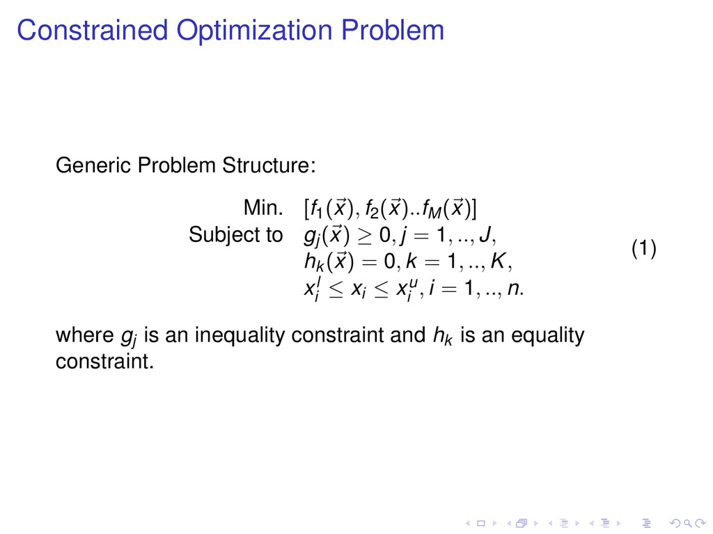
(x)..fM (x)] Subject to gj (x) ≥ 0, j = 1, .., J, hk (x) = 0, k = 1, .., K, xl i ≤ xi ≤ xu i , i = 1, .., n. (1) where gj is an inequality constraint and hk is an equality constraint.
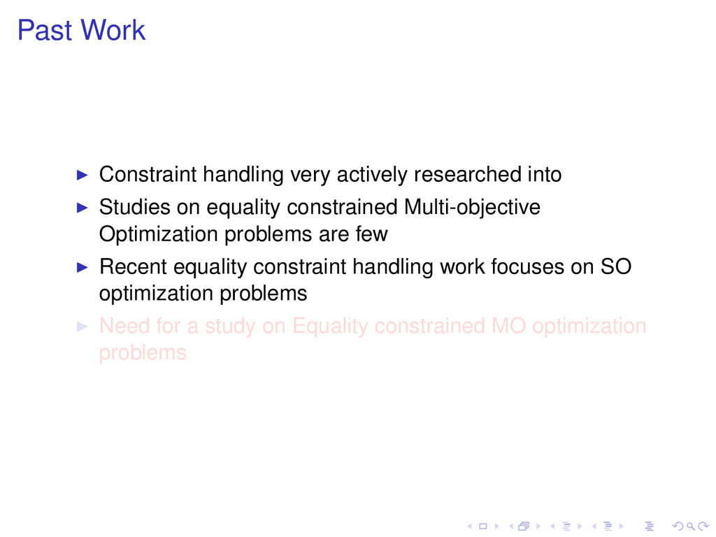
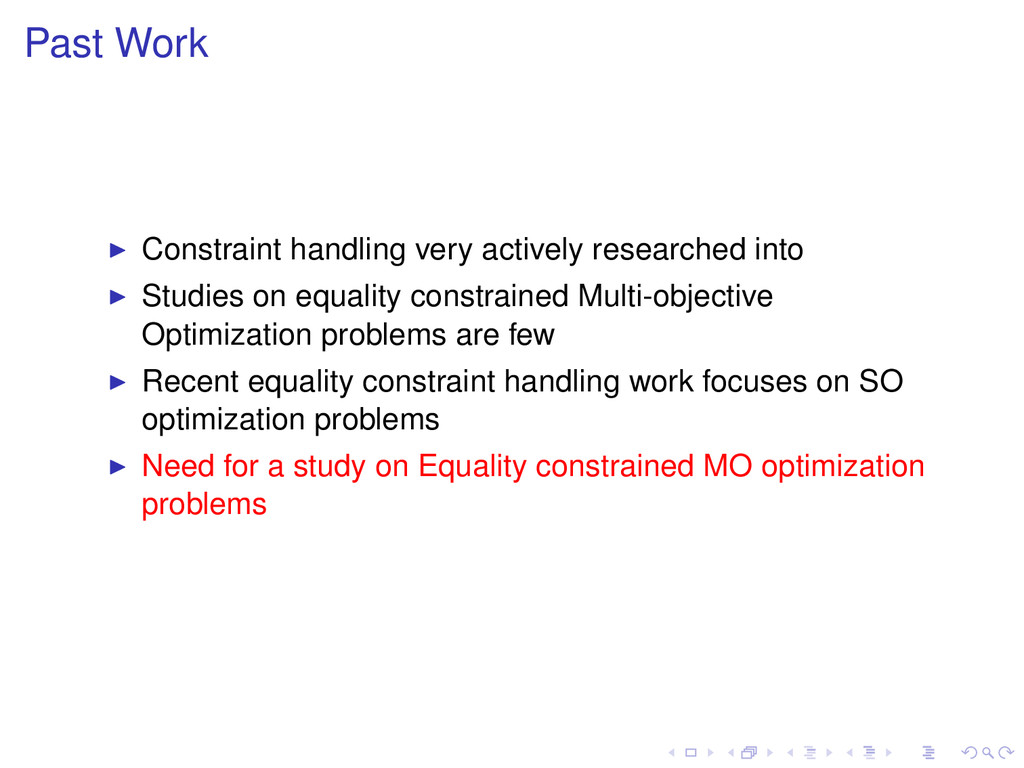
Studies on equality constrained Multi-objective Optimization problems are few ◮ Recent equality constraint handling work focuses on SO optimization problems ◮ Need for a study on Equality constrained MO optimization problems
Studies on equality constrained Multi-objective Optimization problems are few ◮ Recent equality constraint handling work focuses on SO optimization problems ◮ Need for a study on Equality constrained MO optimization problems
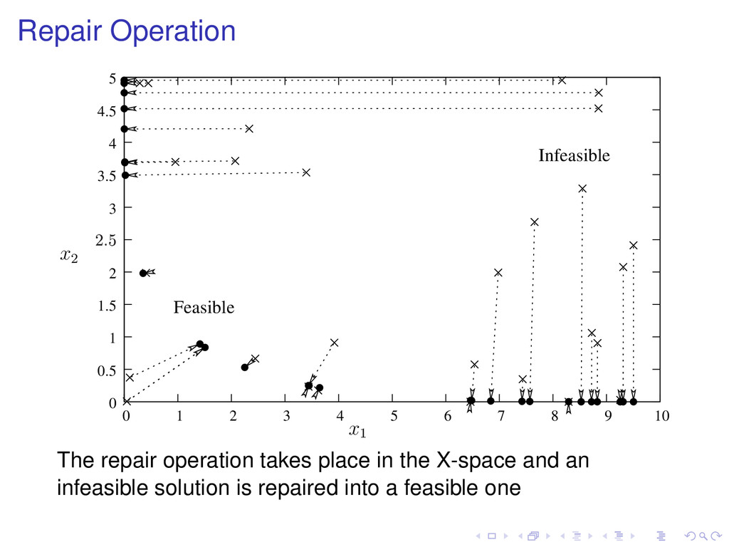
Based Design Optimization X−space O A C D B X* h(x) = 0 ÁÒ × Ð Ö ÓÒ¸ h(x) = 0 U1 ÁÒ × Ð Ö ÓÒ¸ h(x) = 0 X U2 Figure: RIA approach: Finding the nearest feasible point, X∗, which is a candidate solution for repairing the infeasible solution, X.
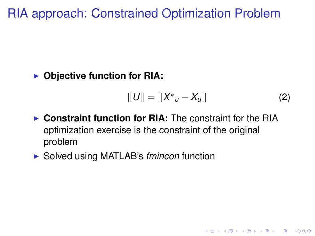
||U|| = ||X∗u − Xu || (2) ◮ Constraint function for RIA: The constraint for the RIA optimization exercise is the constraint of the original problem ◮ Solved using MATLAB’s fmincon function
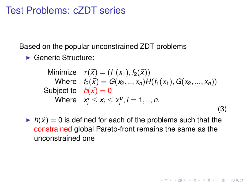
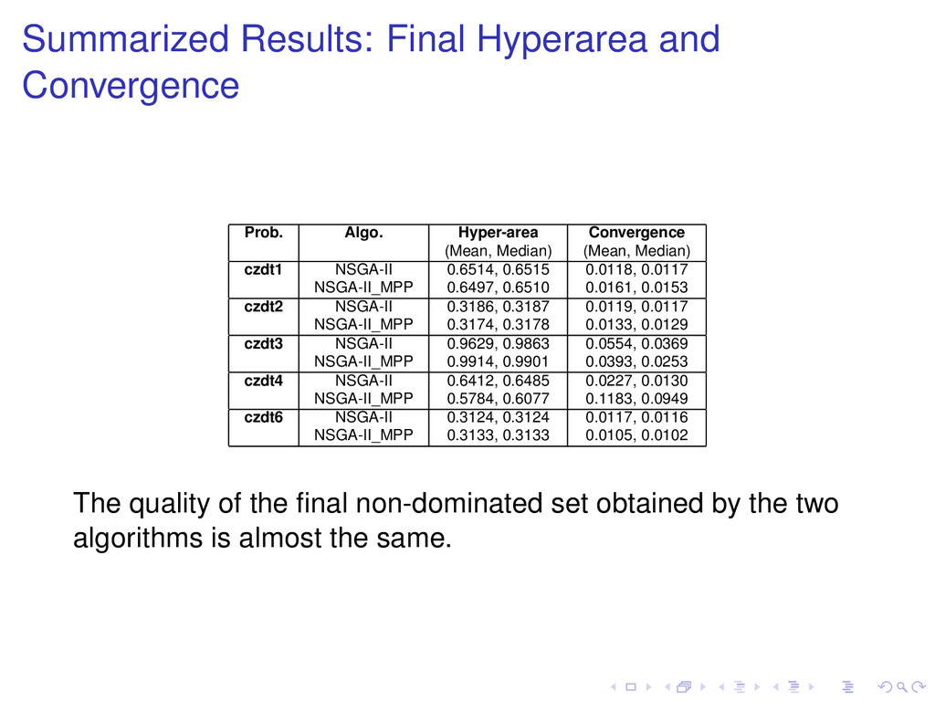
problems ◮ Generic Structure: Minimize τ(x) = (f1 (x1 ), f2 (x)) Where f2 (x) = G(x2 , .., xn )H(f1 (x1 ), G(x2 , ..., xn )) Subject to h(x) = 0 Where xl i ≤ xi ≤ xu i , i = 1, .., n. (3) ◮ h(x) = 0 is defined for each of the problems such that the constrained global Pareto-front remains the same as the unconstrained one
multi-objective optimization, in IEEE Congress of Evolutionary Computation (CEC), (Brisbane, Australia) ◮ Saha, A. and Ray, T. (2012).A repair mechanism for active inequality constraint handling, in IEEE Congress of Evolutionary Computation (CEC),(Brisbane,Australia) ◮ Saha,A. and Ray, T.(2011), Attaining Feasible State in Equality Constrained Optimization Using Genetic Algorithms (Technical Report)