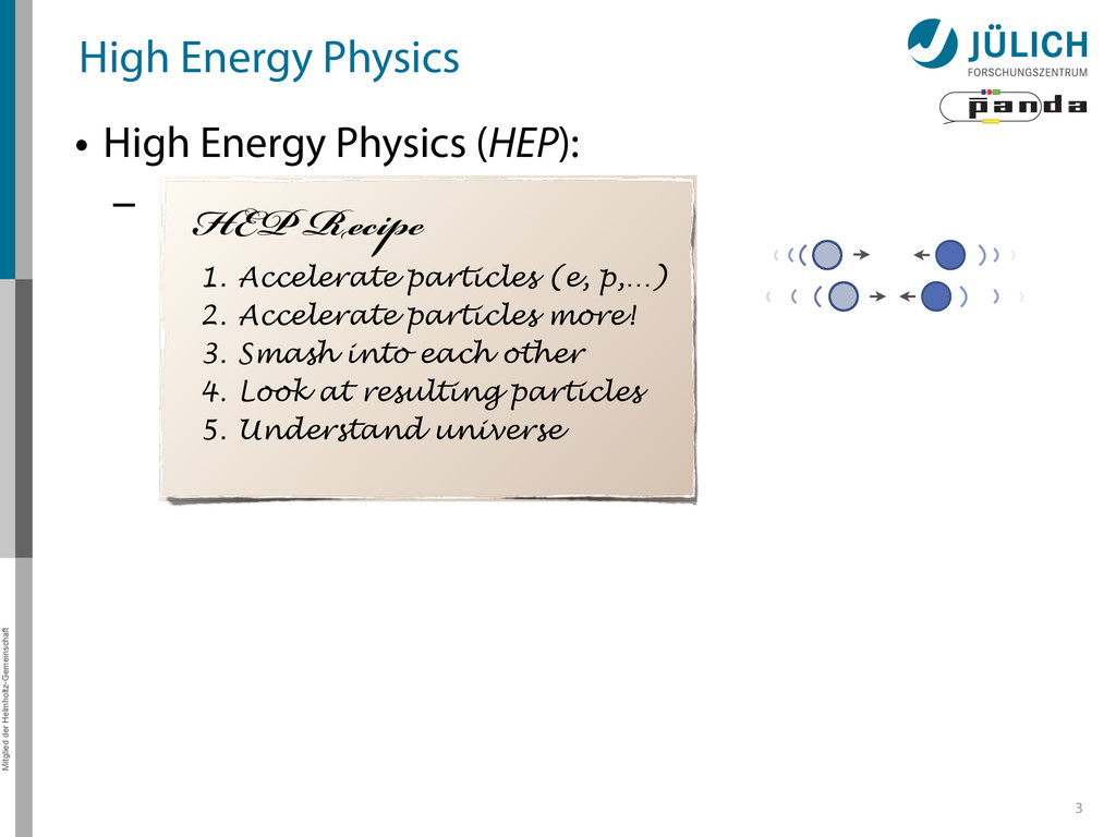
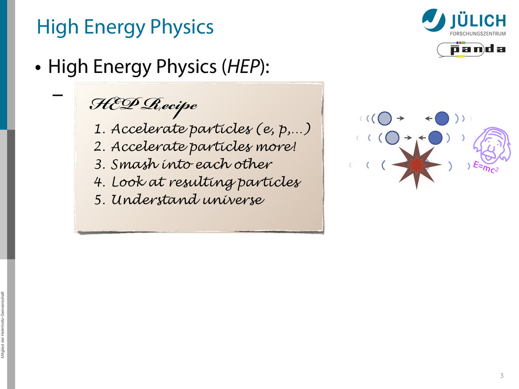
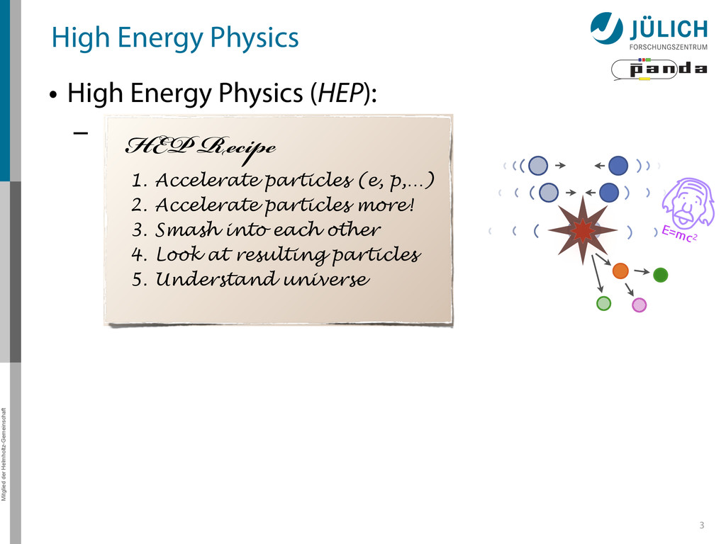
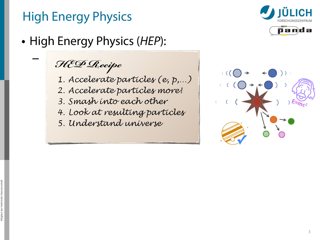
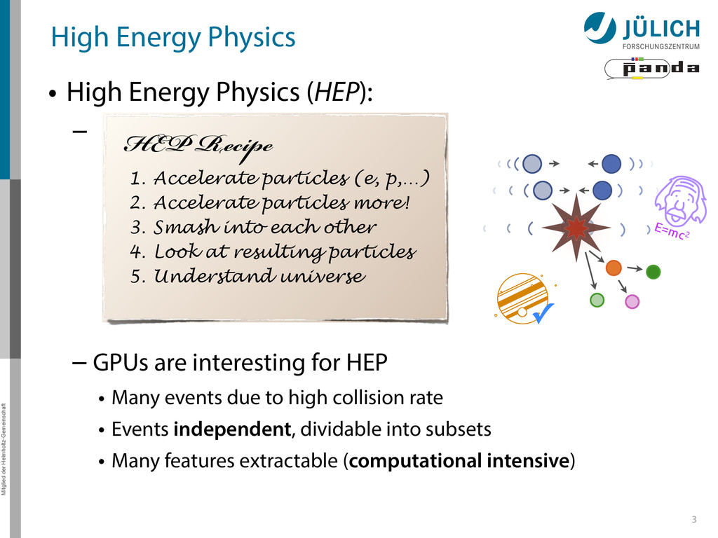
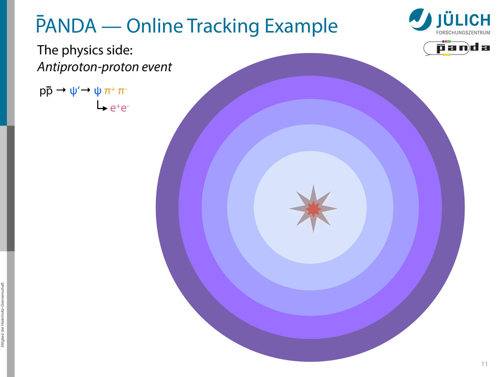
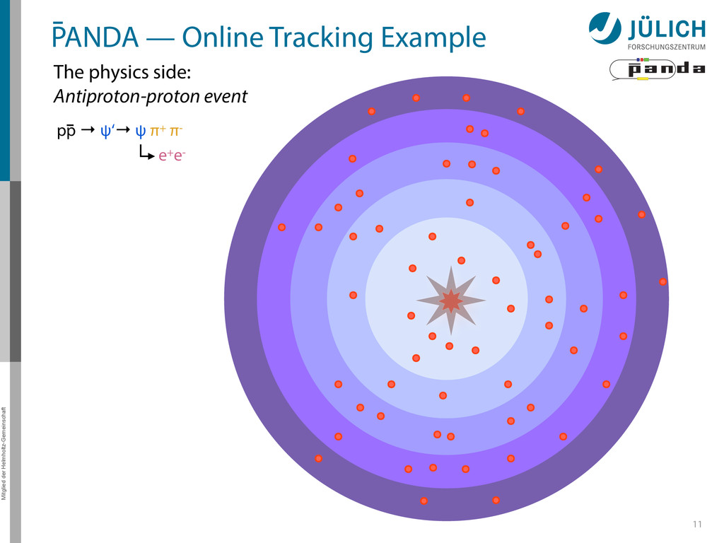
(HEP): – 3 HEP Recipe 1. Accelerate particles (e, p,…) 2. Accelerate particles more! 3. Smash into each other 4. Look at resulting particles 5. Understand universe ✓ – GPUs are interesting for HEP • Many events due to high collision rate • Events independent, dividable into subsets • Many features extractable (computational intensive) E=mc2
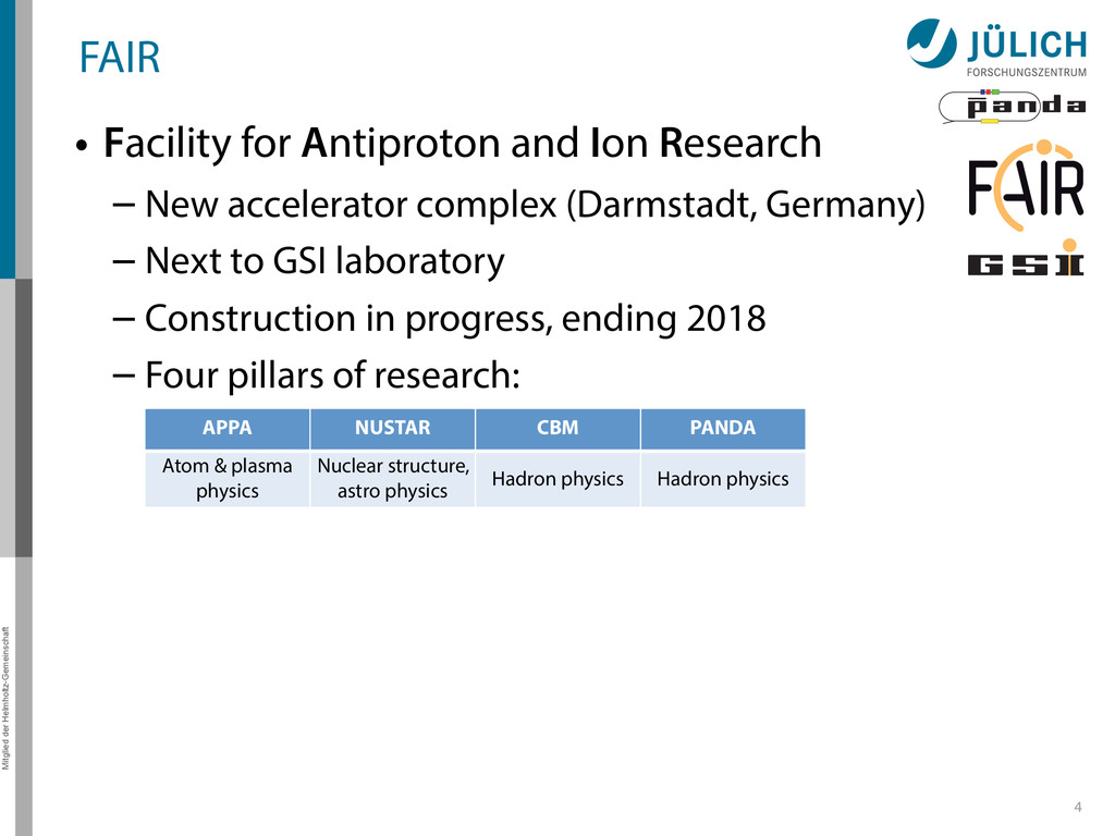
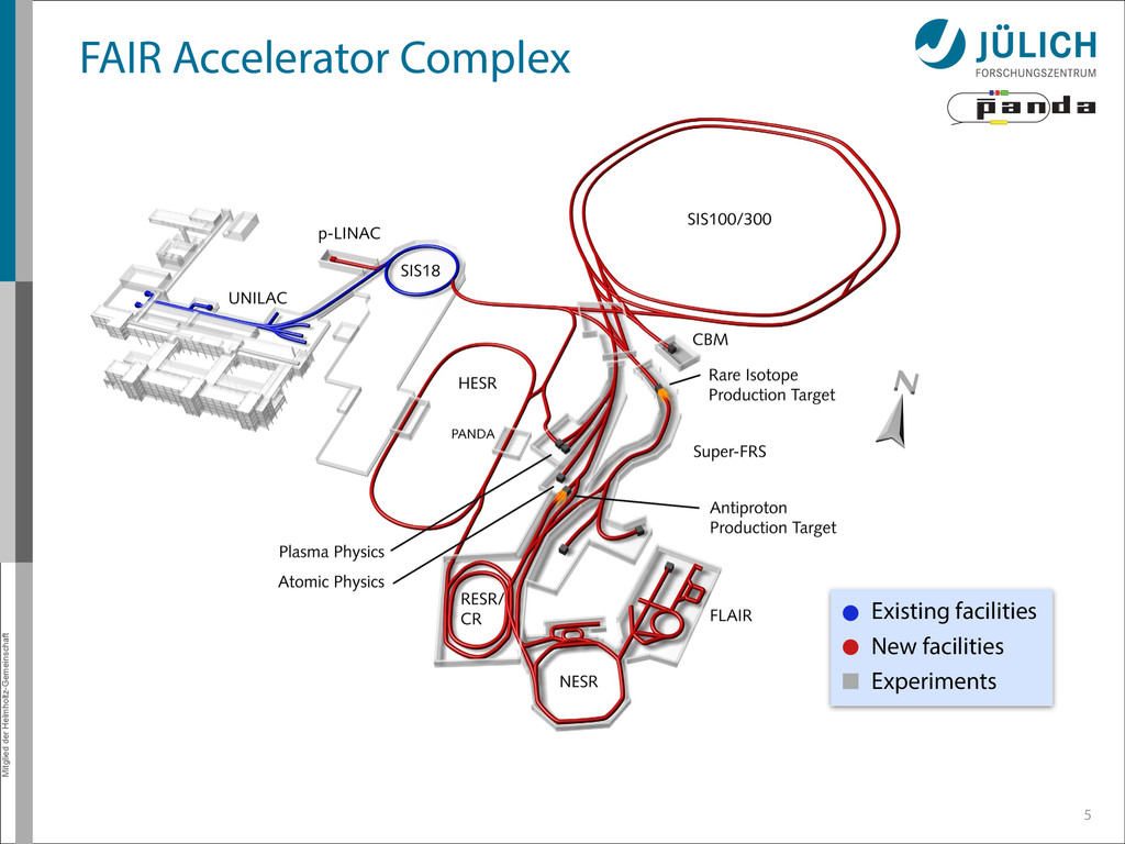
Research – New accelerator complex (Darmstadt, Germany) – Next to GSI laboratory – Construction in progress, ending 2018 – Four pillars of research: 4 APPA NUSTAR CBM PANDA Atom & plasma physics Nuclear structure, astro physics Hadron physics Hadron physics
Research – New accelerator complex (Darmstadt, Germany) – Next to GSI laboratory – Construction in progress, ending 2018 – Four pillars of research: 4 APPA NUSTAR CBM PANDA Atom & plasma physics Nuclear structure, astro physics Hadron physics Hadron physics
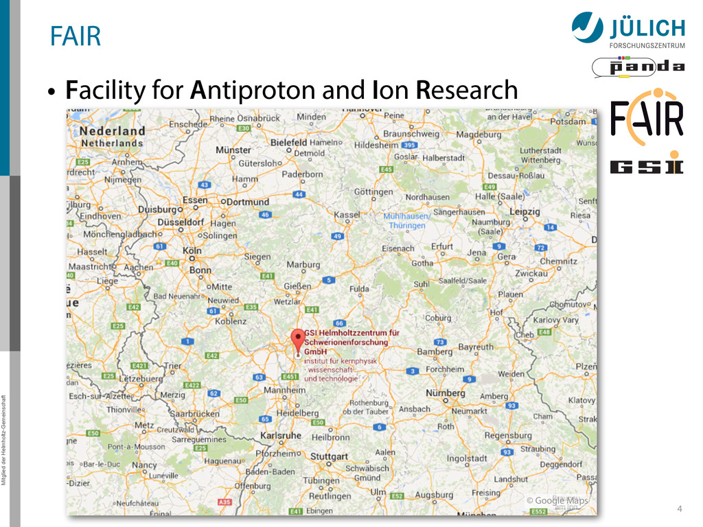
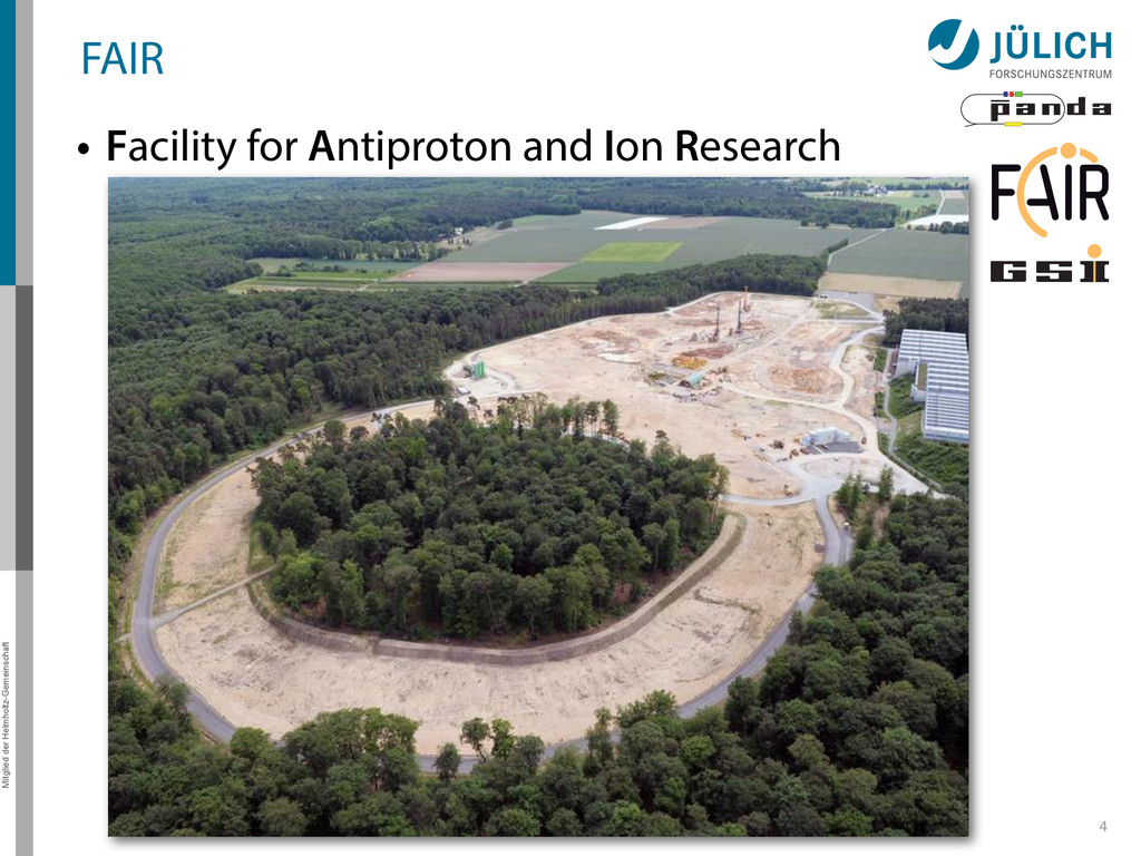
Research – New accelerator complex (Darmstadt, Germany) – Next to GSI laboratory – Construction in progress, ending 2018 – Four pillars of research: 4 APPA NUSTAR CBM PANDA Atom & plasma physics Nuclear structure, astro physics Hadron physics Hadron physics fair-center.eu
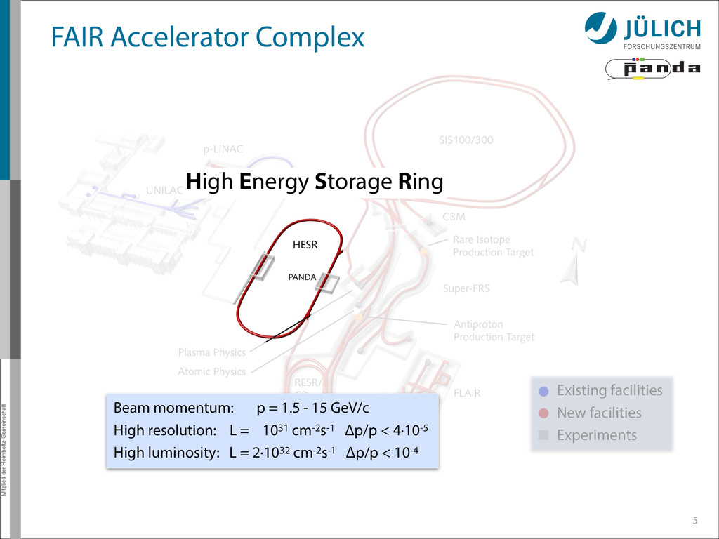
Existing facilities New facilities Experiments Beam momentum: p = 1.5 - 15 GeV/c High resolution: L = 1031 cm-2s-1 Δp/p < 4·10-5 High luminosity: L = 2·1032 cm-2s-1 Δp/p < 10-4 High Energy Storage Ring
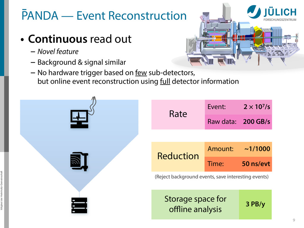
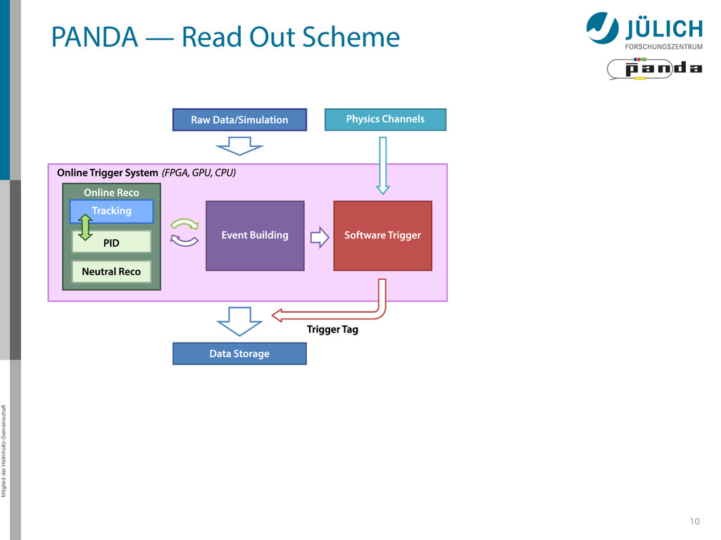
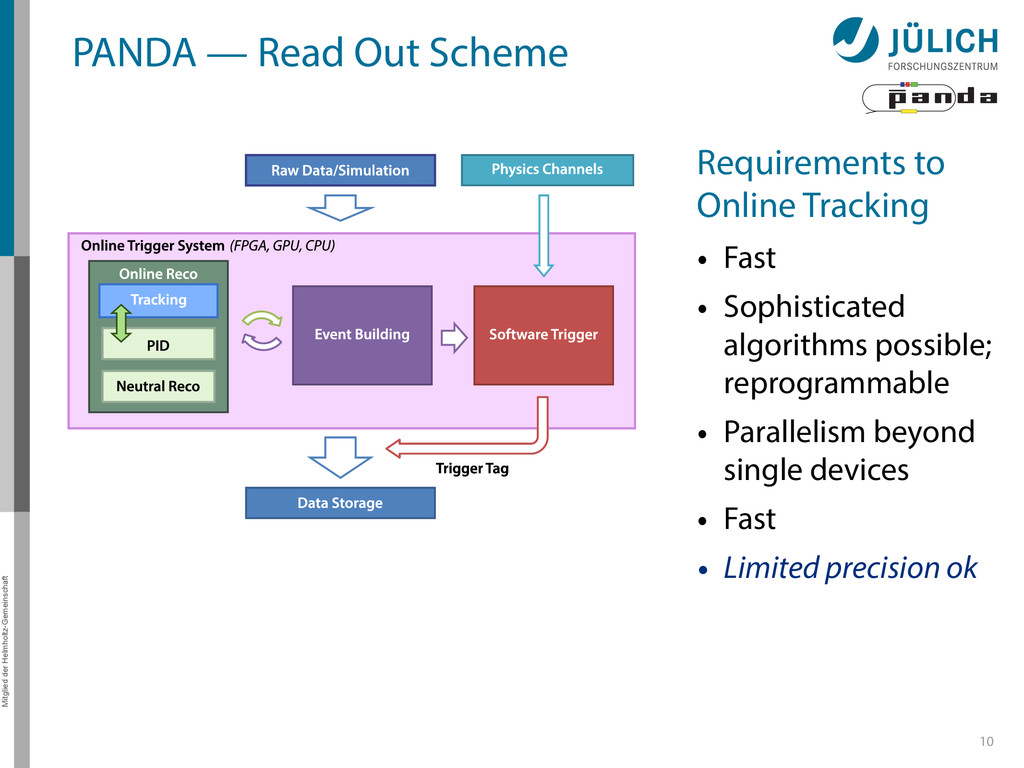
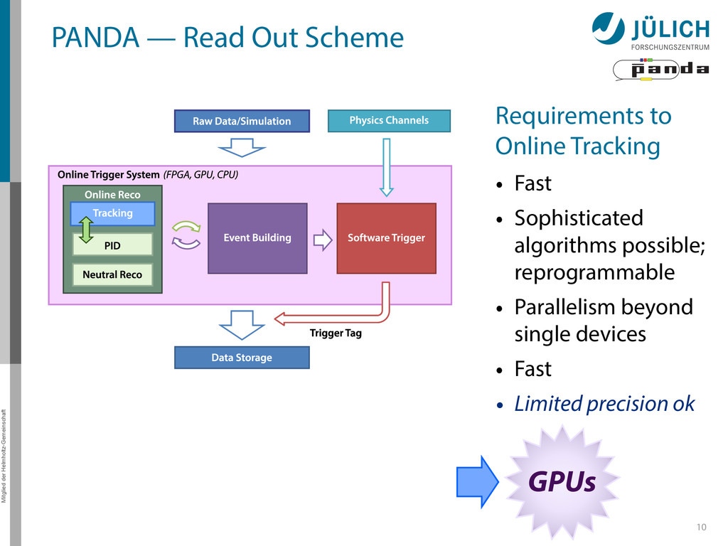
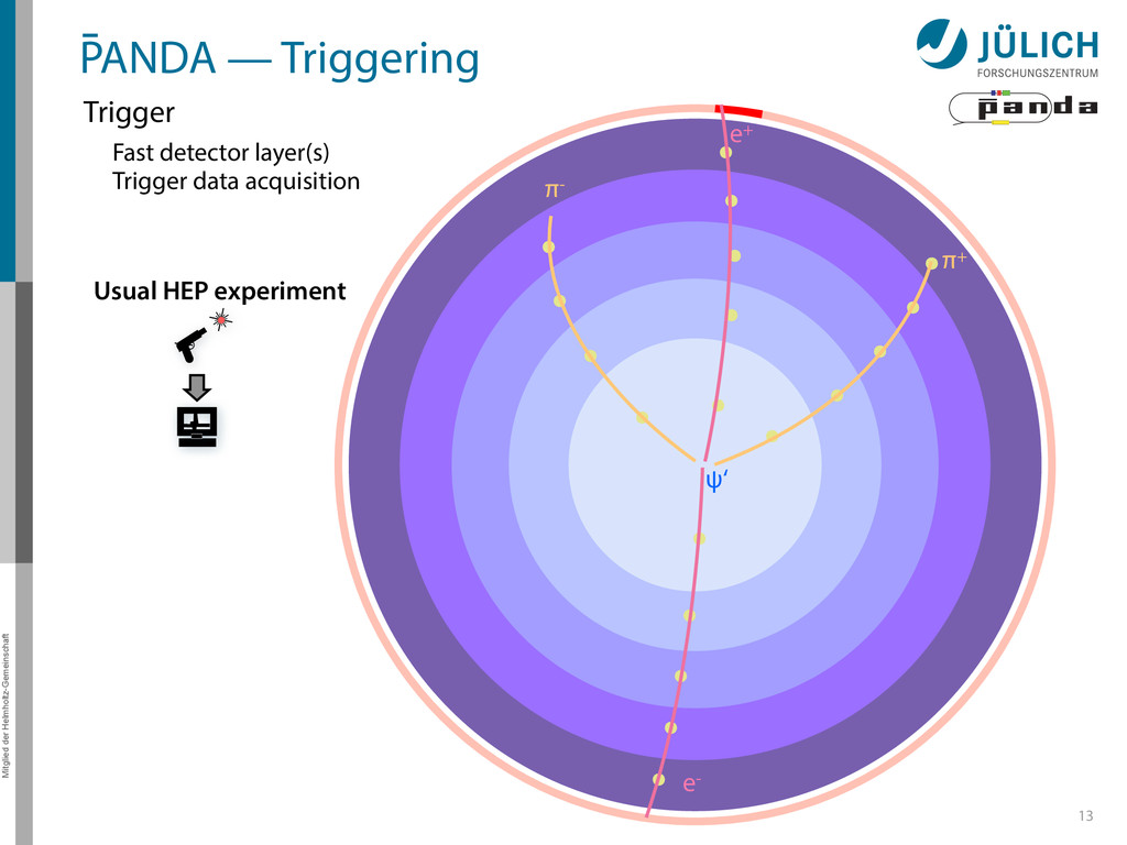
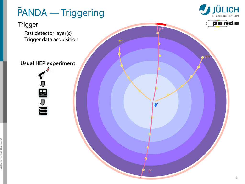
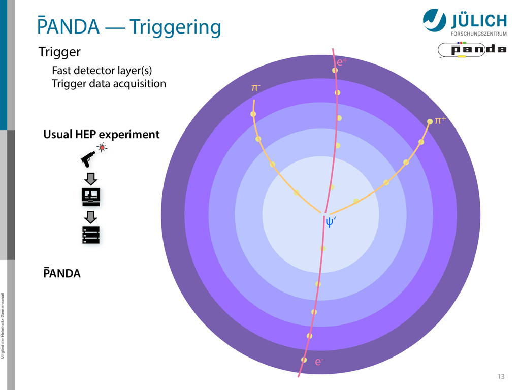
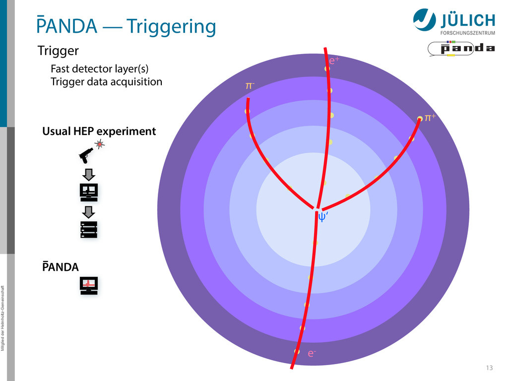
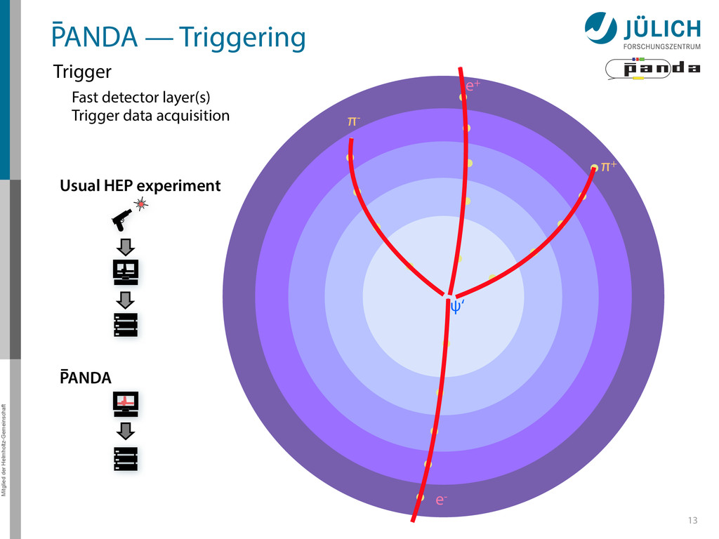
out – Novel feature – Background & signal similar – No hardware trigger based on few sub-detectors, but online event reconstruction using full detector information 9 (Reject background events, save interesting events) Reduction Amount: Time: ~1/1000 50 ns/evt Storage space for offline analysis 3 PB/y Event: Raw data: 2 × 10⁷/s 200 GB/s Rate
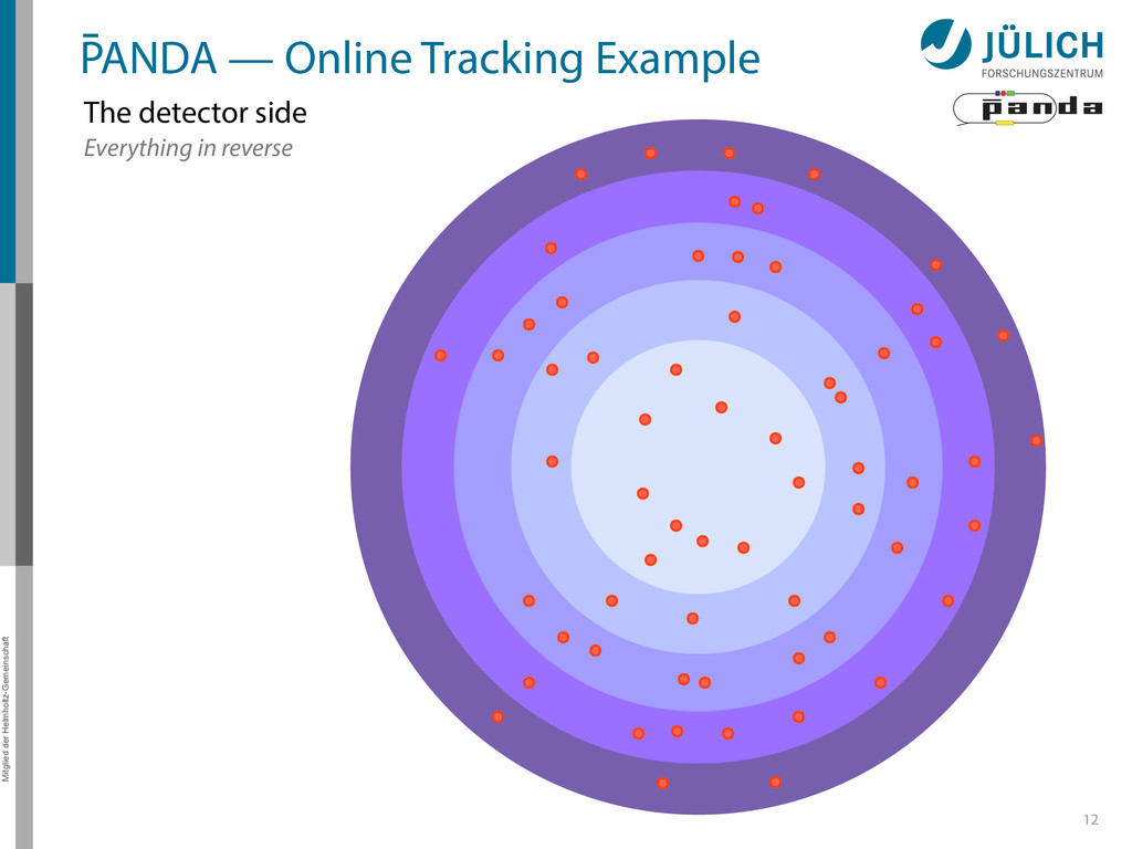
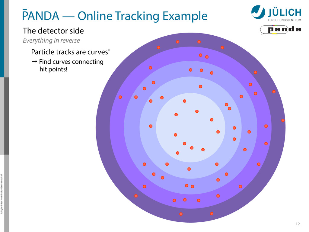
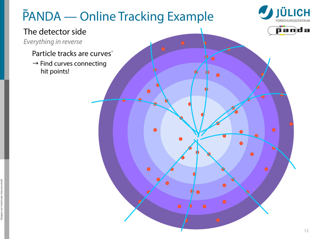
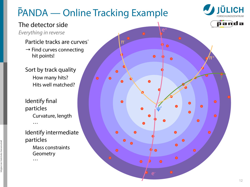
detector side Everything in reverse Particle tracks are curves* → Find curves connecting hit points! Sort by track quality Hits well matched? How many hits?
detector side Everything in reverse Particle tracks are curves* → Find curves connecting hit points! Sort by track quality Hits well matched? How many hits?
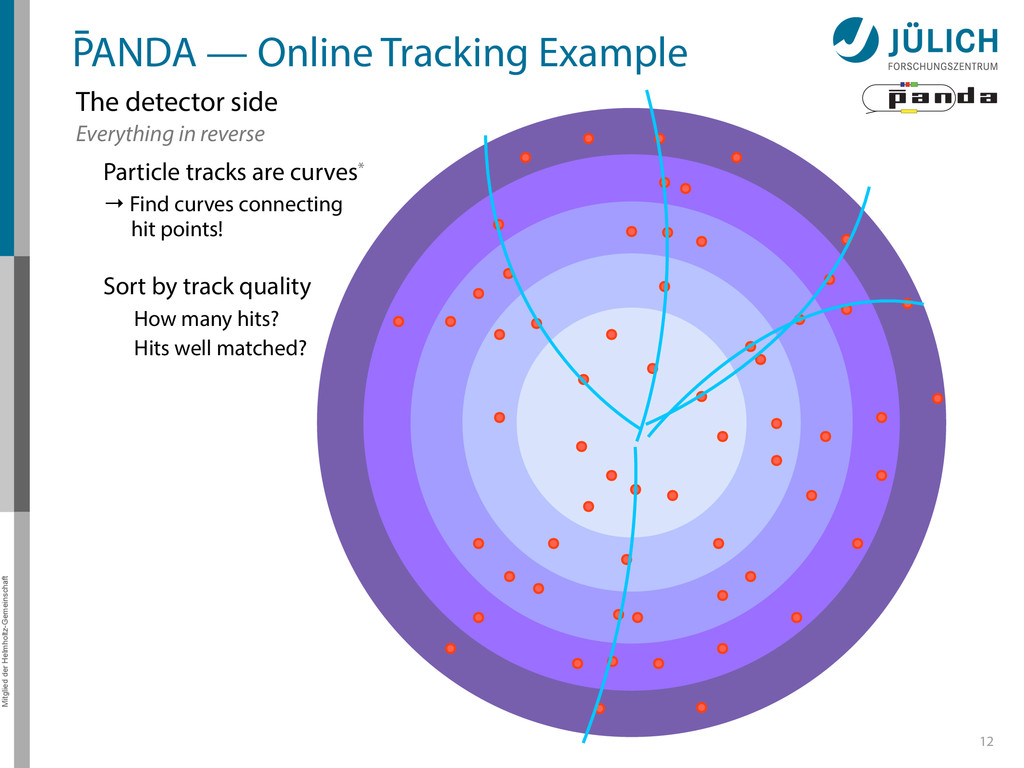
detector side Everything in reverse Particle tracks are curves* → Find curves connecting hit points! Sort by track quality Hits well matched? How many hits? Identify final particles Curvature, length …
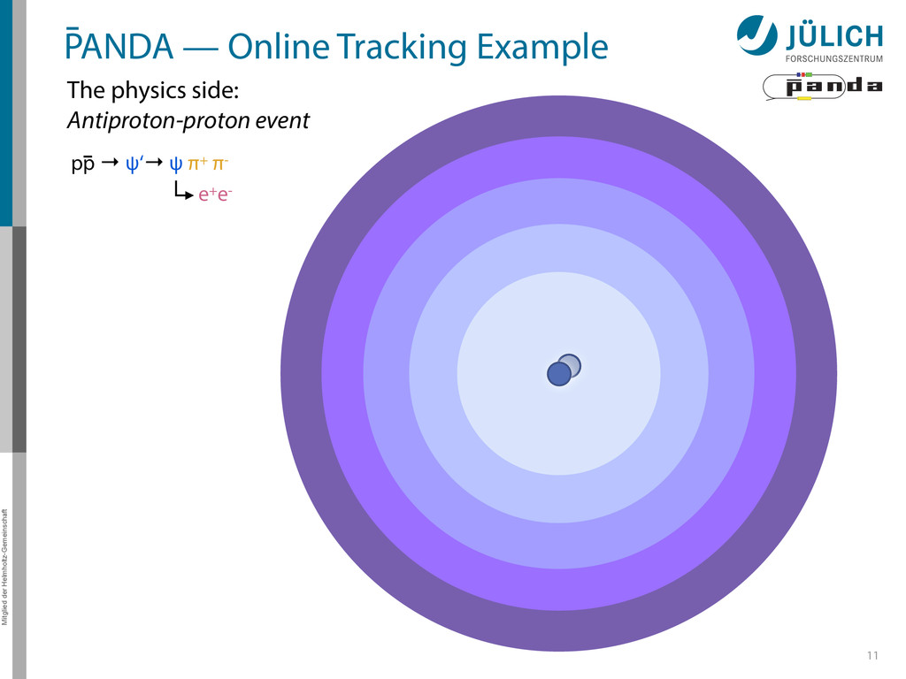
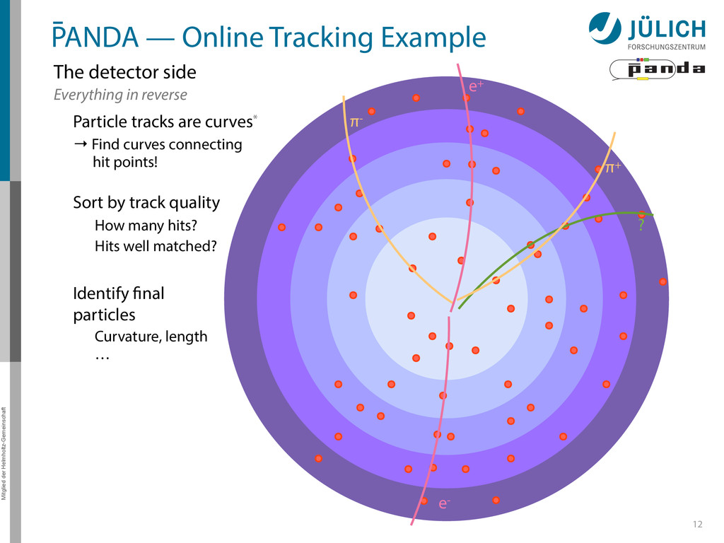
detector side Everything in reverse Particle tracks are curves* → Find curves connecting hit points! Sort by track quality Hits well matched? How many hits? Identify final particles Curvature, length … π+ π- e+ e- ?
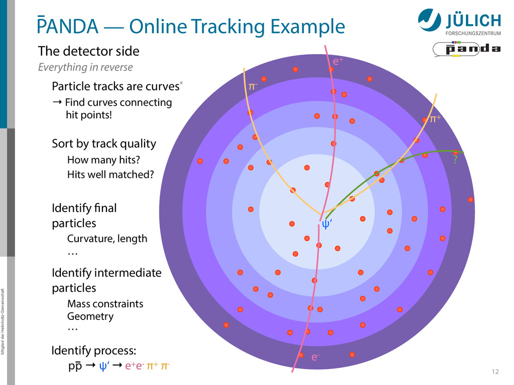
detector side Everything in reverse Particle tracks are curves* → Find curves connecting hit points! Sort by track quality Hits well matched? How many hits? Identify final particles Curvature, length … Identify intermediate particles Mass constraints Geometry … π+ π- e+ e- ? ψ‘
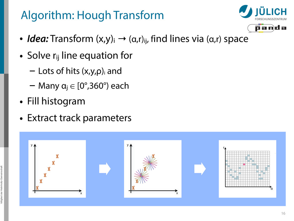
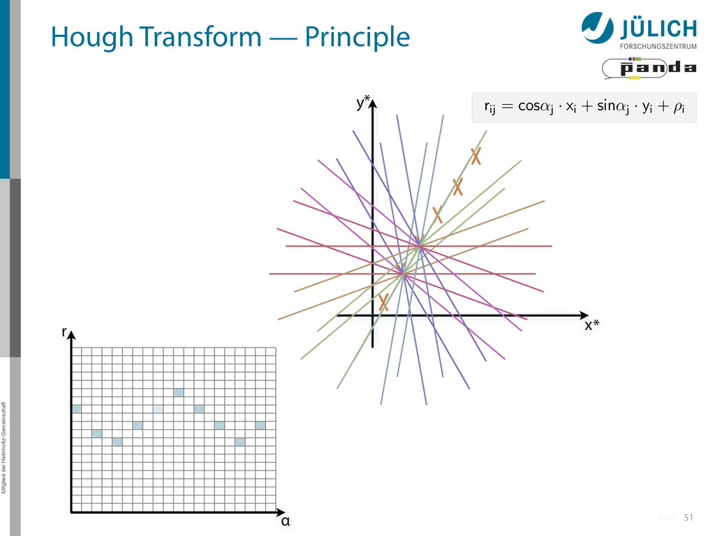
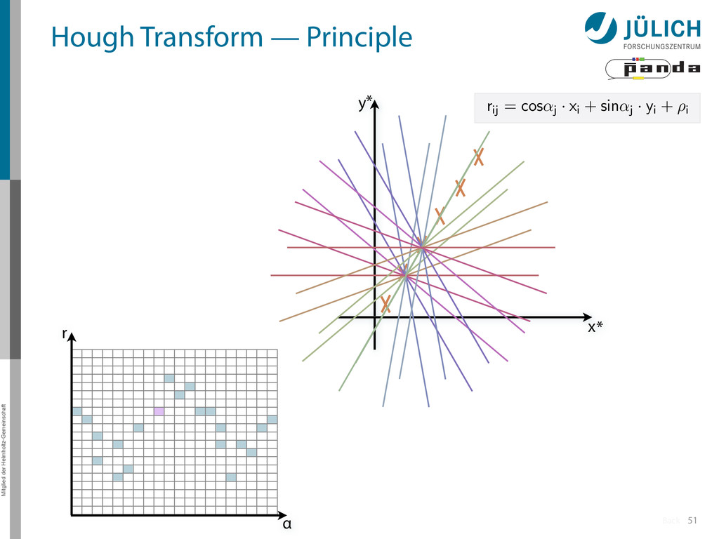
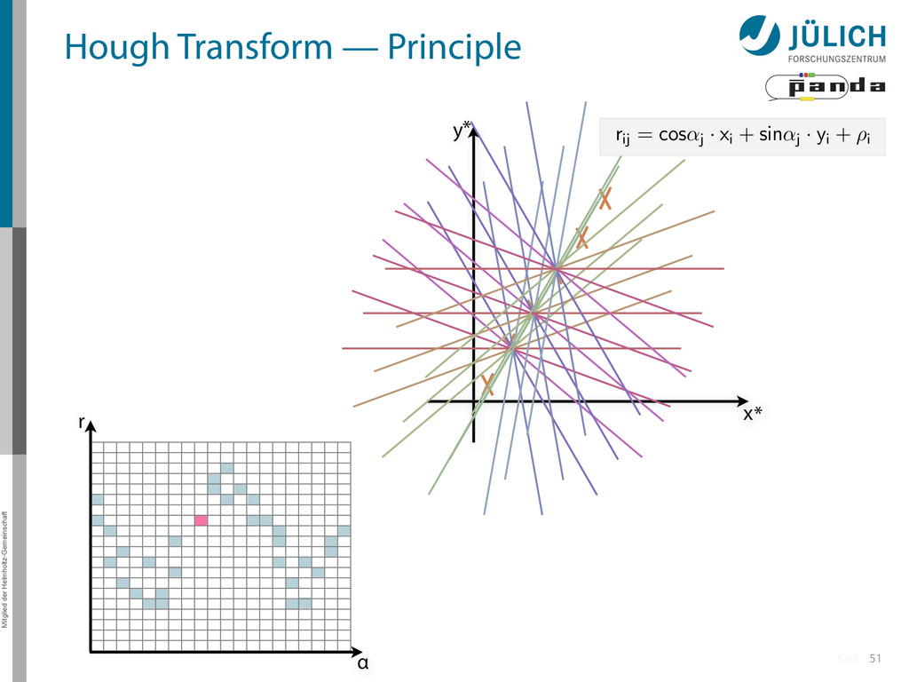
→ (α,r)ij, find lines via (α,r) space • Solve rij line equation for – Lots of hits (x,y,ρ)i and – Many αj ∈ [0°,360°) each • Fill histogram • Extract track parameters 16 x y x y Mitglied der Helmholtz-Gemeinschaft Hough Transform — Princip → Bin giv r α
→ (α,r)ij, find lines via (α,r) space • Solve rij line equation for – Lots of hits (x,y,ρ)i and – Many αj ∈ [0°,360°) each • Fill histogram • Extract track parameters 16 rij = cos ↵j · xi + sin ↵j · yi + ⇢i i: ~100 hits/event (STT) j: every 0.2° rij: 180 000 x y x y Mitglied der Helmholtz-Gemeinschaft Hough Transform — Princip → Bin giv r α
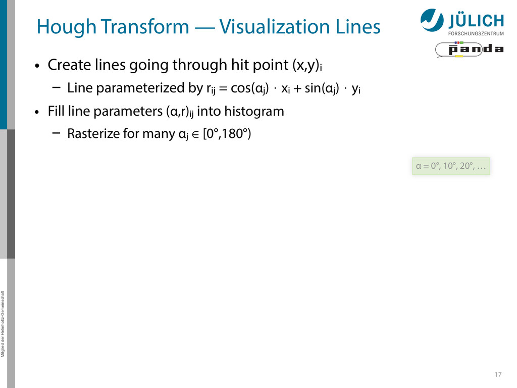
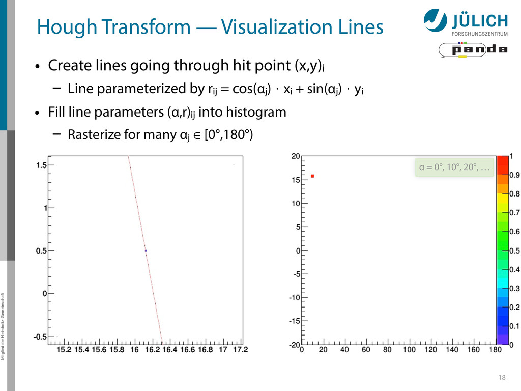
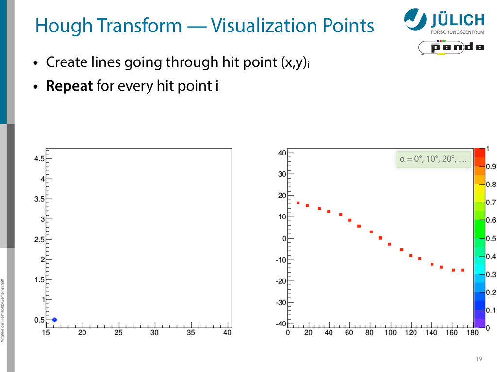
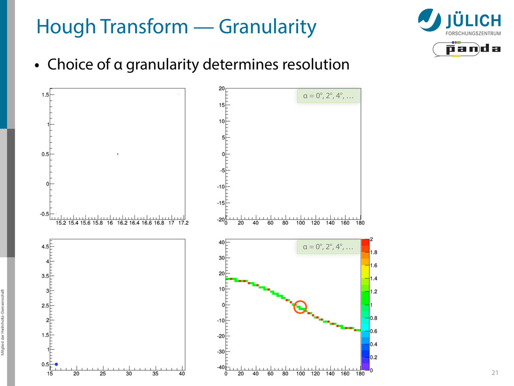
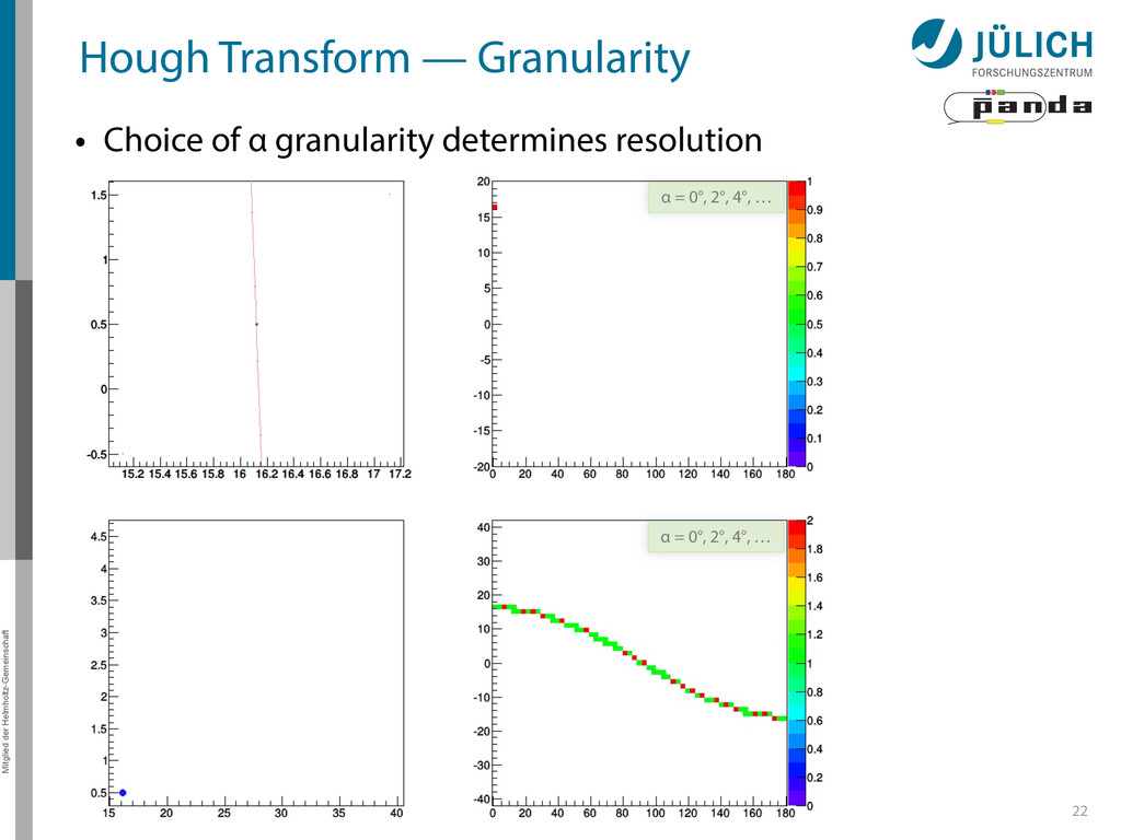
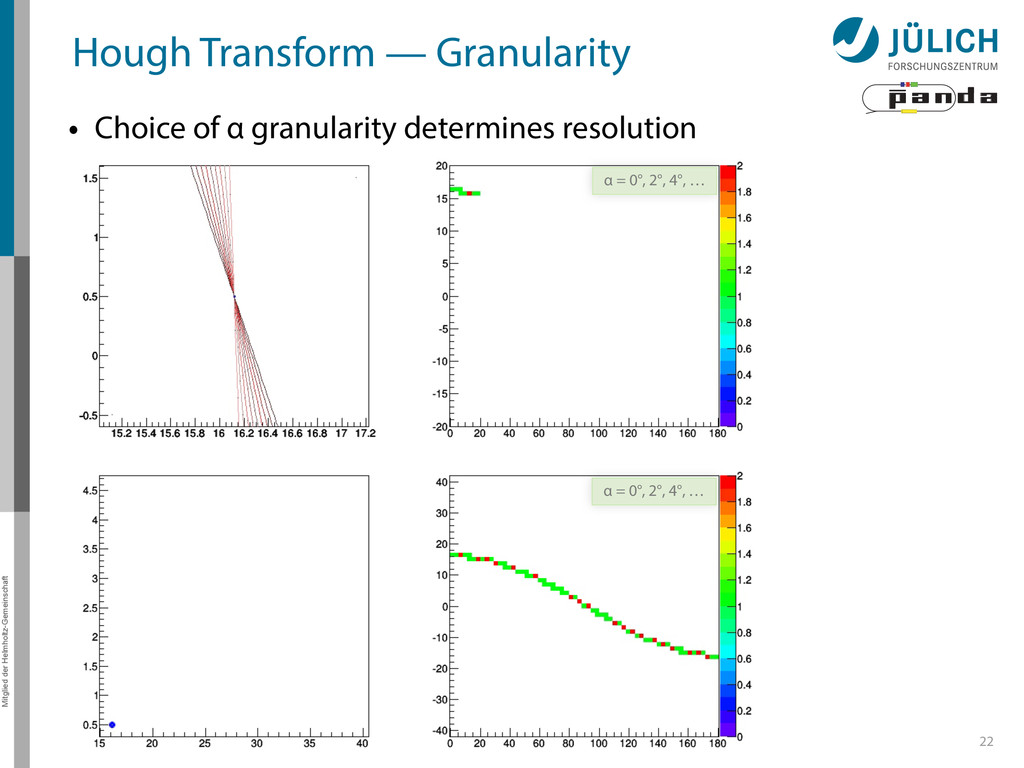
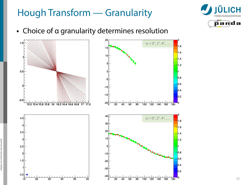
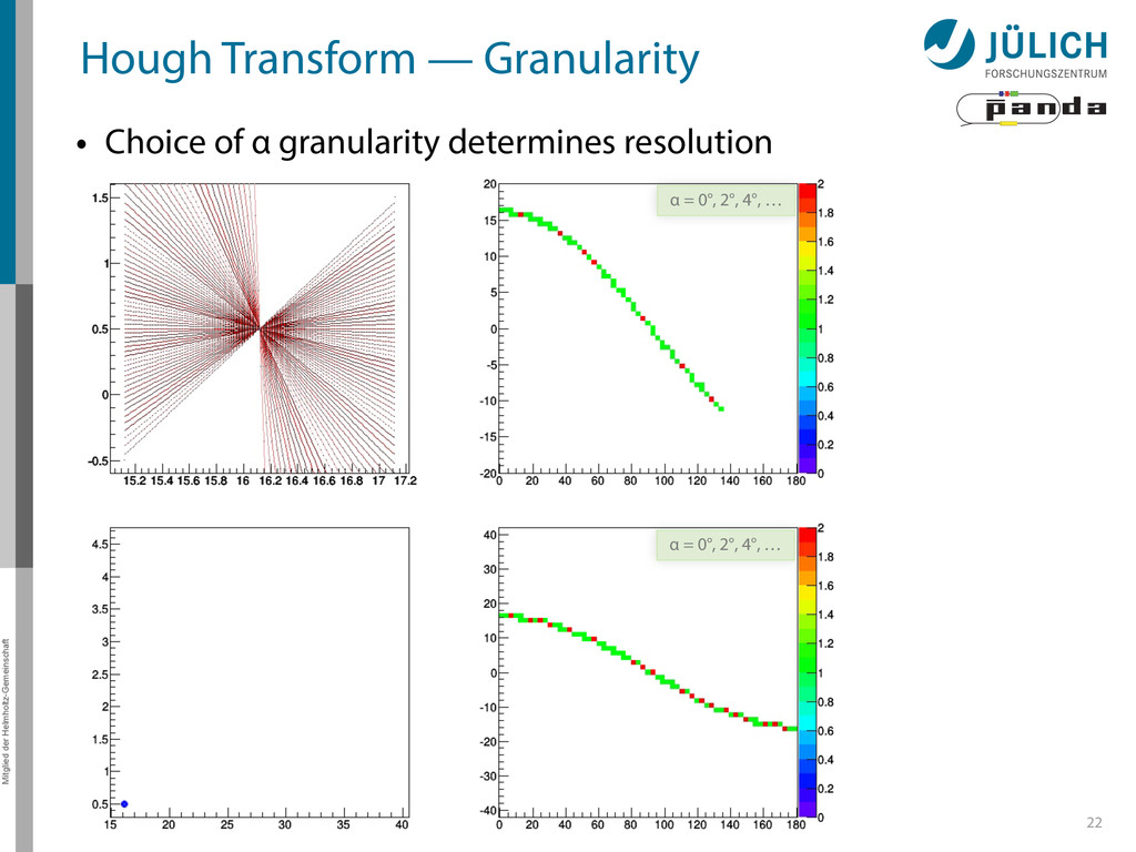
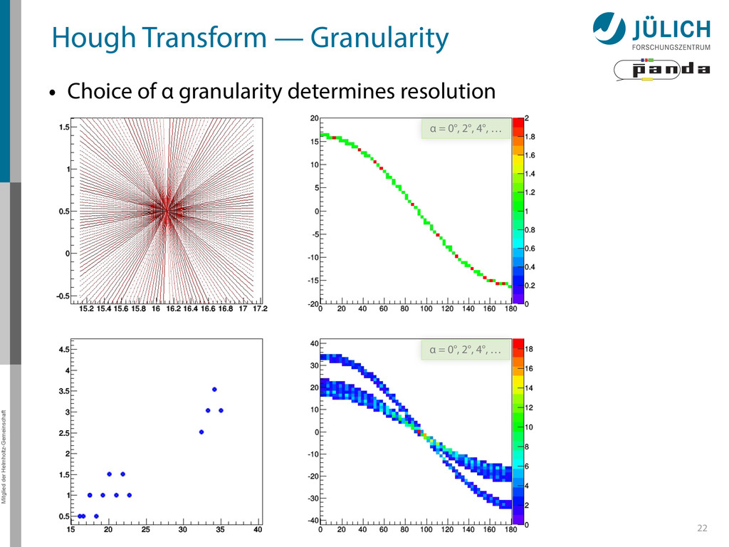
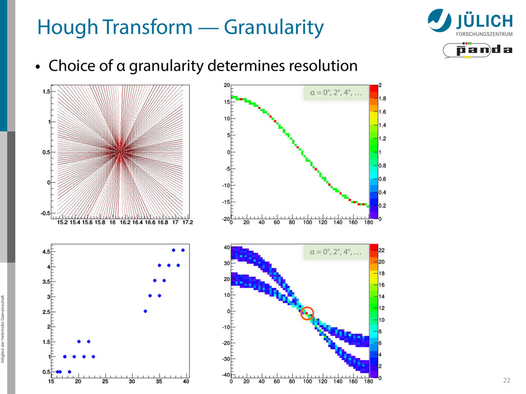
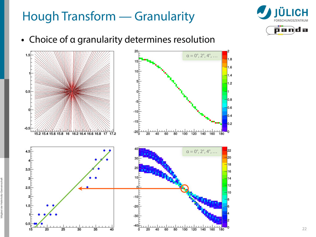
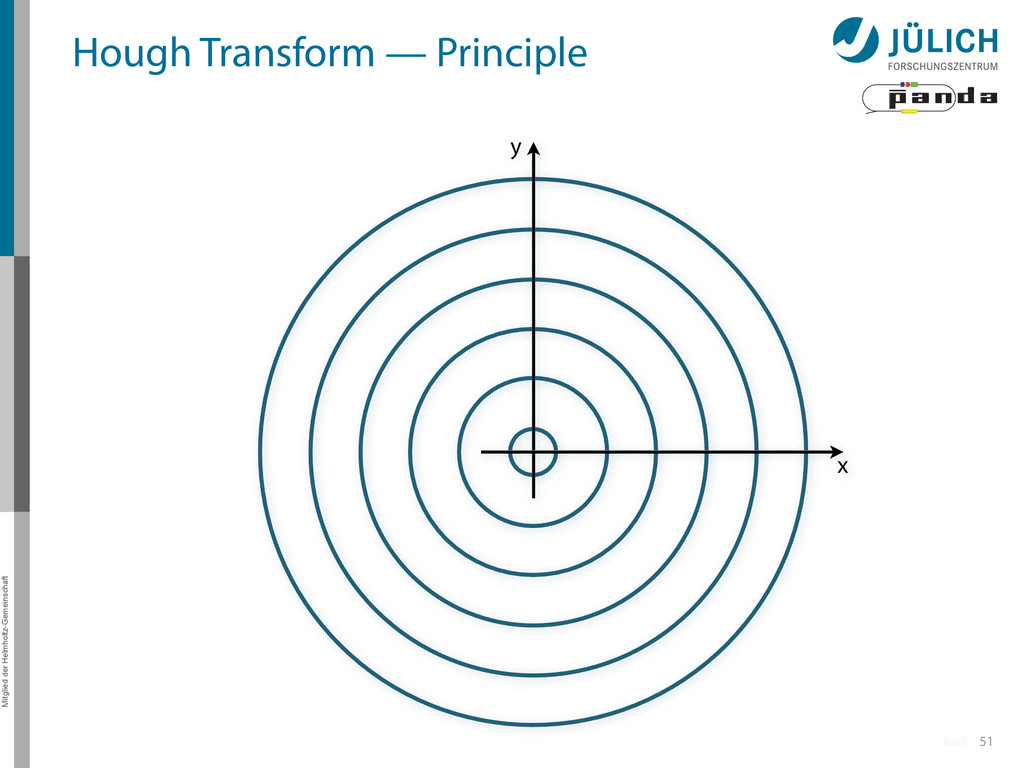
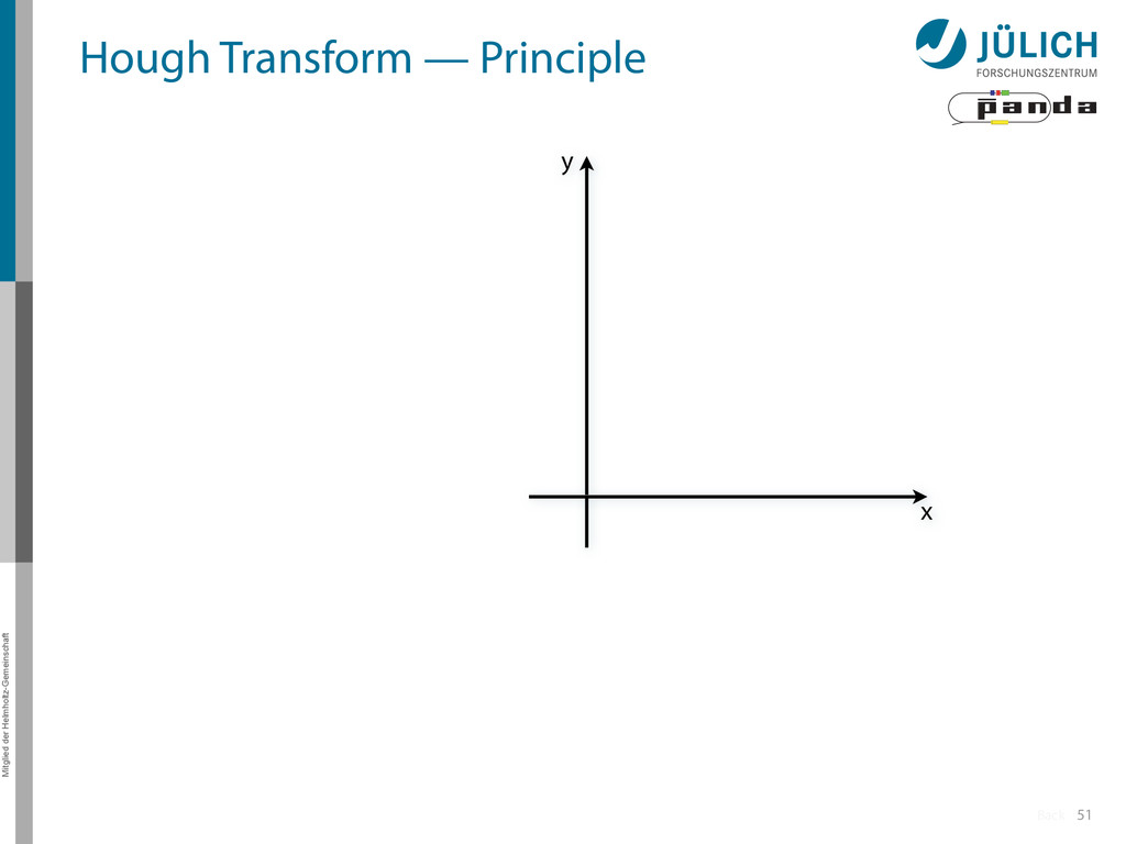
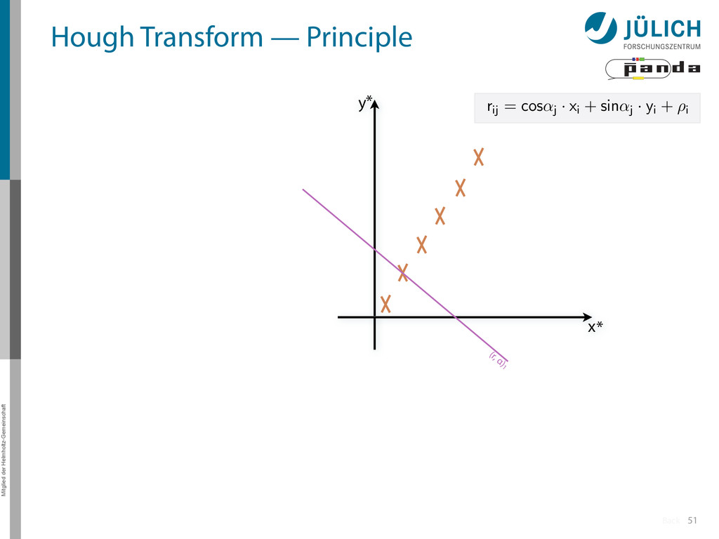
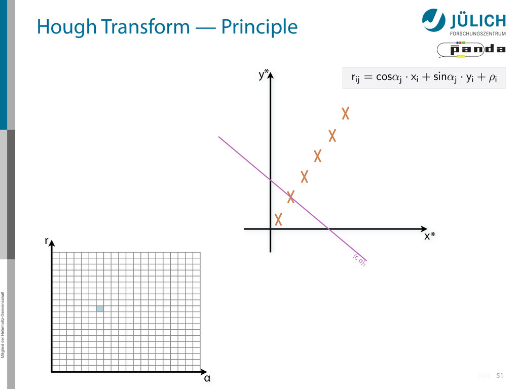
Create lines going through hit point (x,y)i – Line parameterized by rij = cos(αj) ⋅ xi + sin(αj) ⋅ yi • Fill line parameters (α,r)ij into histogram – Rasterize for many αj ∈ [0°,180°) α = 0°, 10°, 20°, …
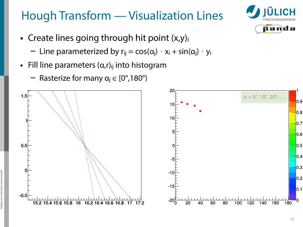
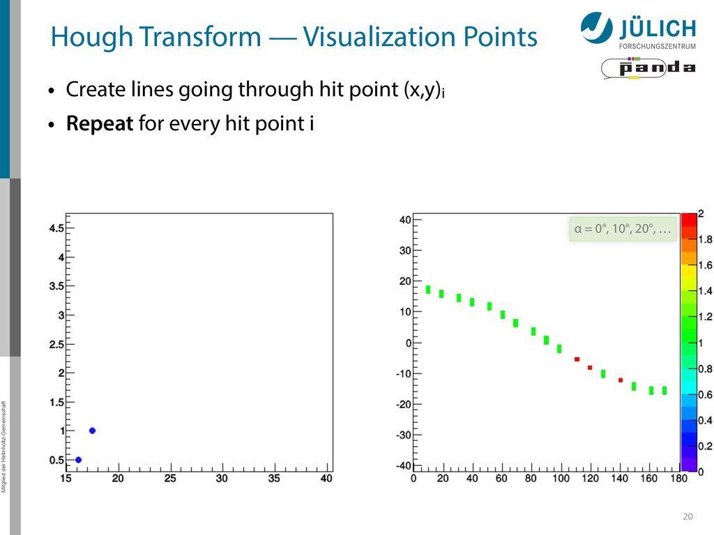
Create lines going through hit point (x,y)i – Line parameterized by rij = cos(αj) ⋅ xi + sin(αj) ⋅ yi • Fill line parameters (α,r)ij into histogram – Rasterize for many αj ∈ [0°,180°) α = 0°, 10°, 20°, …
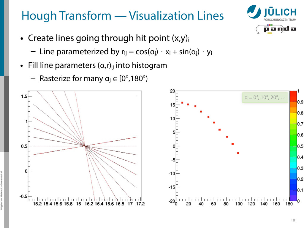
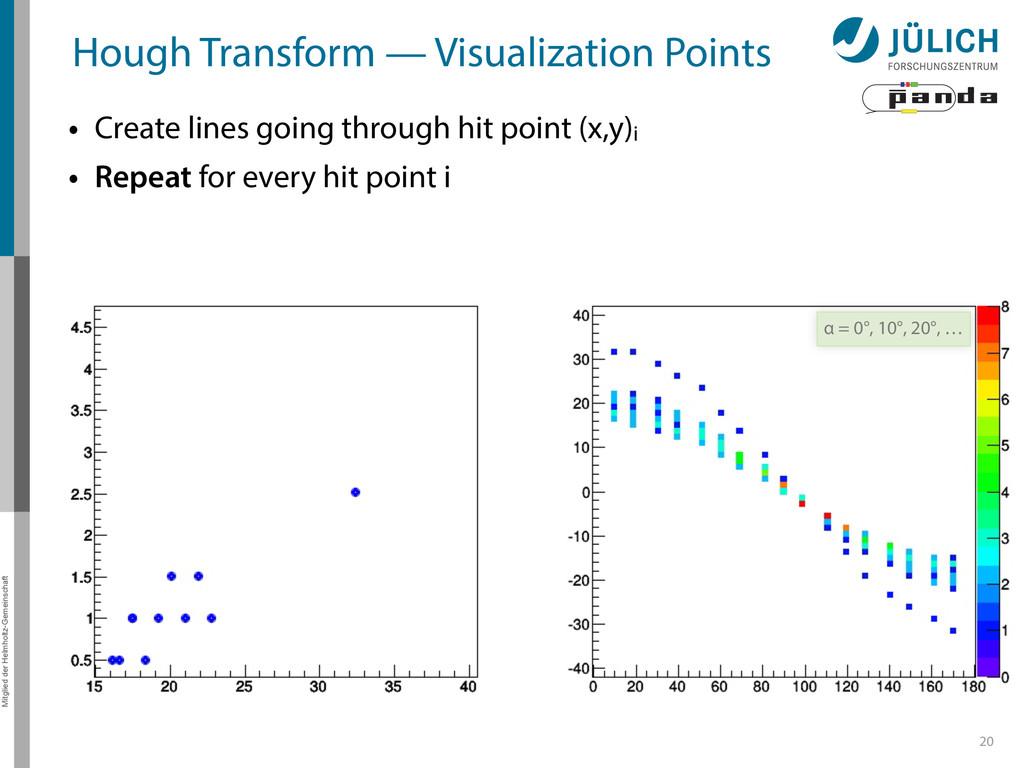
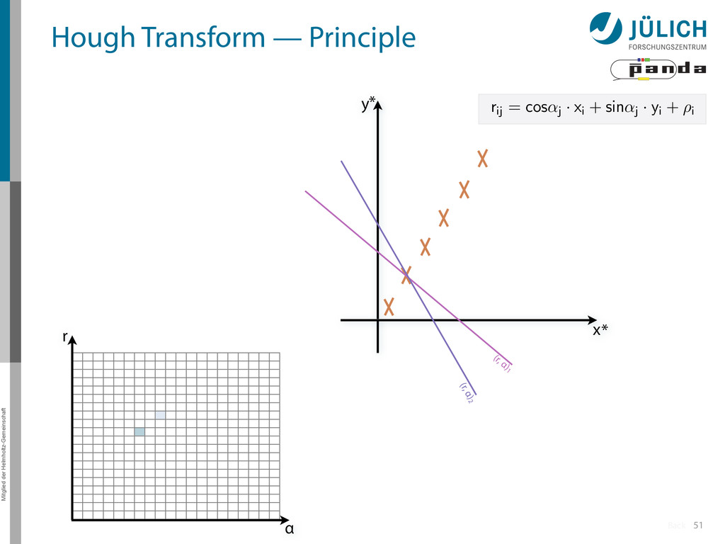
Create lines going through hit point (x,y)i – Line parameterized by rij = cos(αj) ⋅ xi + sin(αj) ⋅ yi • Fill line parameters (α,r)ij into histogram – Rasterize for many αj ∈ [0°,180°) α = 0°, 10°, 20°, …
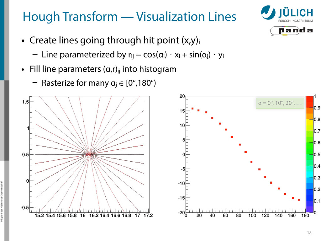
Create lines going through hit point (x,y)i – Line parameterized by rij = cos(αj) ⋅ xi + sin(αj) ⋅ yi • Fill line parameters (α,r)ij into histogram – Rasterize for many αj ∈ [0°,180°) α = 0°, 10°, 20°, …
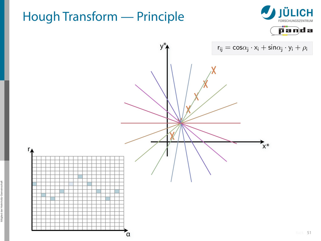
Create lines going through hit point (x,y)i – Line parameterized by rij = cos(αj) ⋅ xi + sin(αj) ⋅ yi • Fill line parameters (α,r)ij into histogram – Rasterize for many αj ∈ [0°,180°) α = 0°, 10°, 20°, …
Create lines going through hit point (x,y)i – Line parameterized by rij = cos(αj) ⋅ xi + sin(αj) ⋅ yi • Fill line parameters (α,r)ij into histogram – Rasterize for many αj ∈ [0°,180°) α = 0°, 10°, 20°, …
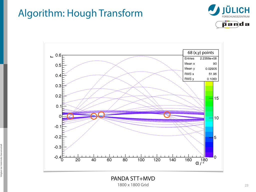
140 160 180 Hough transformed -0.4 -0.3 -0.2 -0.1 0 0.1 0.2 0.3 0.4 0.5 0.6 0 Entries 2.2356e+08 Mean x 90 Mean y 0.02905 RMS x 51.96 RMS y 0.1063 0 5 10 15 20 25 0 Entries 2.2356e+08 Mean x 90 Mean y 0.02905 RMS x 51.96 RMS y 0.1063 1800 x 1800 Grid PANDA STT+MVD Mitglied der Helmholtz-Gemeinschaft 23 68 (x,y) points r α Algorithm: Hough Transform
140 160 180 Hough transformed -0.4 -0.3 -0.2 -0.1 0 0.1 0.2 0.3 0.4 0.5 0.6 0 Entries 2.2356e+08 Mean x 90 Mean y 0.02905 RMS x 51.96 RMS y 0.1063 0 5 10 15 20 25 0 Entries 2.2356e+08 Mean x 90 Mean y 0.02905 RMS x 51.96 RMS y 0.1063 1800 x 1800 Grid PANDA STT+MVD Mitglied der Helmholtz-Gemeinschaft 23 68 (x,y) points r α Algorithm: Hough Transform
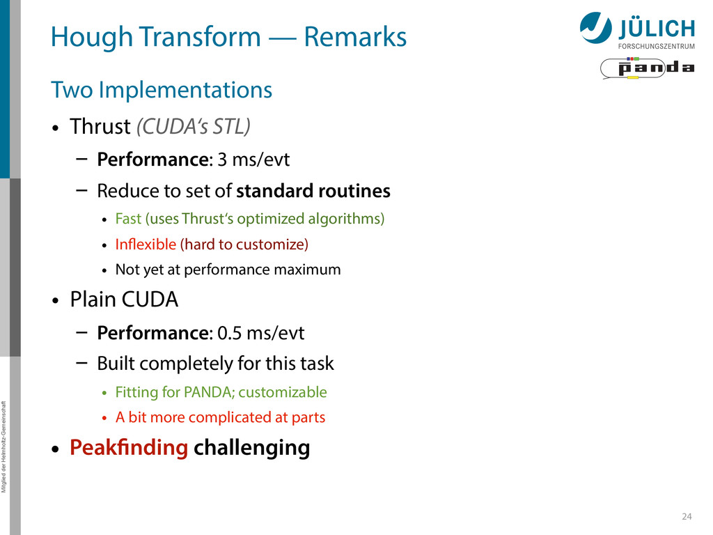
Thrust (CUDA‘s STL) – Performance: 3 ms/evt – Reduce to set of standard routines • Fast (uses Thrust‘s optimized algorithms) • Inflexible (hard to customize) • Not yet at performance maximum • Plain CUDA – Performance: 0.5 ms/evt – Built completely for this task • Fitting for PANDA; customizable • A bit more complicated at parts • 24 Peakfinding challenging
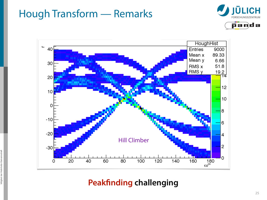
α 0 20 40 60 80 100 120 140 160 180 r -30 -20 -10 0 10 20 30 40 HoughHist Entries 9000 Mean x 89.33 Mean y 6.66 RMS x 51.8 RMS y 19.2 0 2 4 6 8 10 12 14 16 18 HoughHist Entries 9000 Mean x 89.33 Mean y 6.66 RMS x 51.8 RMS y 19.2 HT histogram Hill Climber Peakfinding challenging
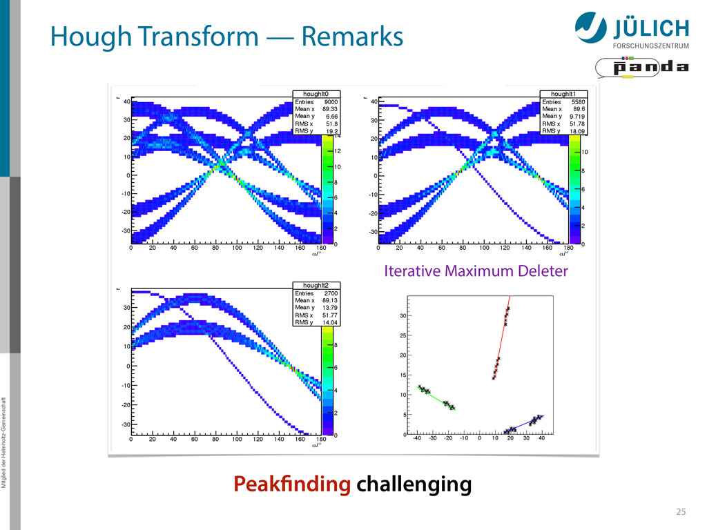
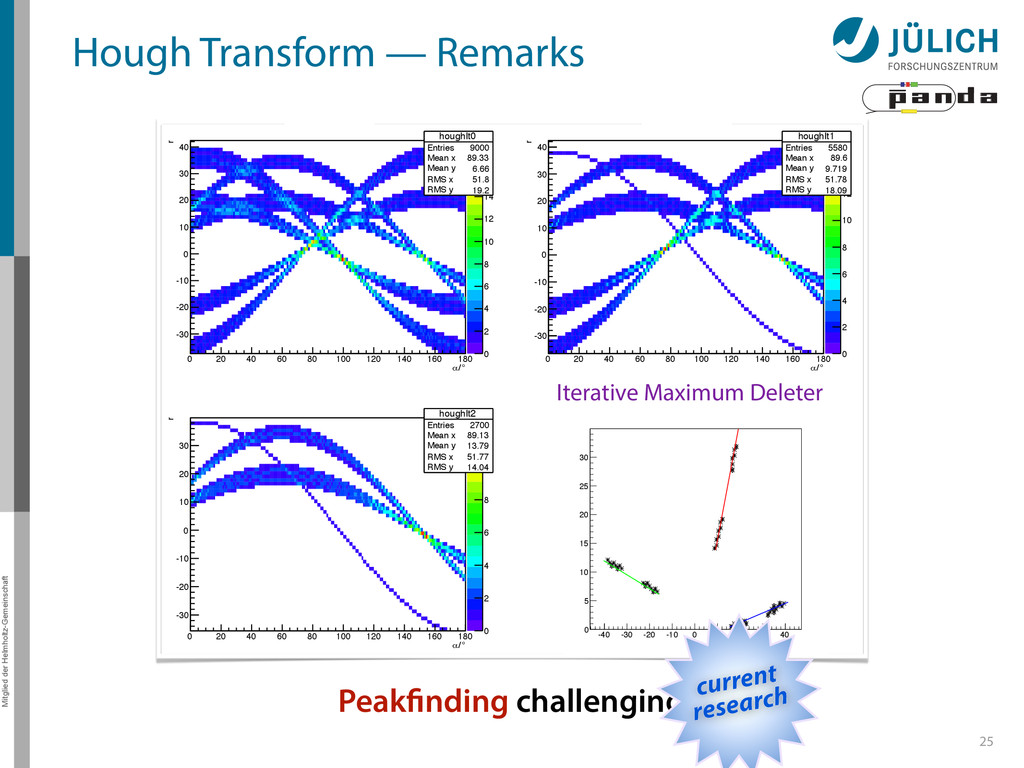
α 0 20 40 60 80 100 120 140 160 180 r -30 -20 -10 0 10 20 30 40 houghIt0 Entries 9000 Mean x 89.33 Mean y 6.66 RMS x 51.8 RMS y 19.2 0 2 4 6 8 10 12 14 16 18 houghIt0 Entries 9000 Mean x 89.33 Mean y 6.66 RMS x 51.8 RMS y 19.2 HT histogram ° / α 0 20 40 60 80 100 120 140 160 180 r -30 -20 -10 0 10 20 30 40 houghIt1 Entries 5580 Mean x 89.6 Mean y 9.719 RMS x 51.78 RMS y 18.09 0 2 4 6 8 10 12 14 16 houghIt1 Entries 5580 Mean x 89.6 Mean y 9.719 RMS x 51.78 RMS y 18.09 HT histogram ° / α 0 20 40 60 80 100 120 140 160 180 r -30 -20 -10 0 10 20 30 houghIt2 Entries 2700 Mean x 89.13 Mean y 13.79 RMS x 51.77 RMS y 14.04 0 2 4 6 8 10 12 houghIt2 Entries 2700 Mean x 89.13 Mean y 13.79 RMS x 51.77 RMS y 14.04 HT histogram -40 -30 -20 -10 0 10 20 30 40 0 5 10 15 20 25 30 Iterative Maximum Deleter Peakfinding challenging current research
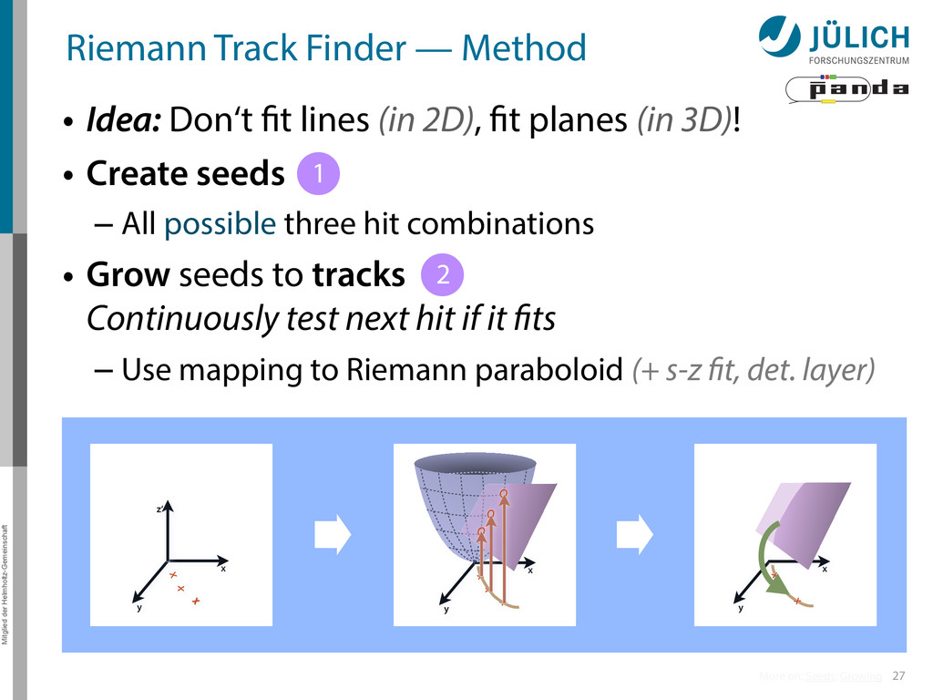
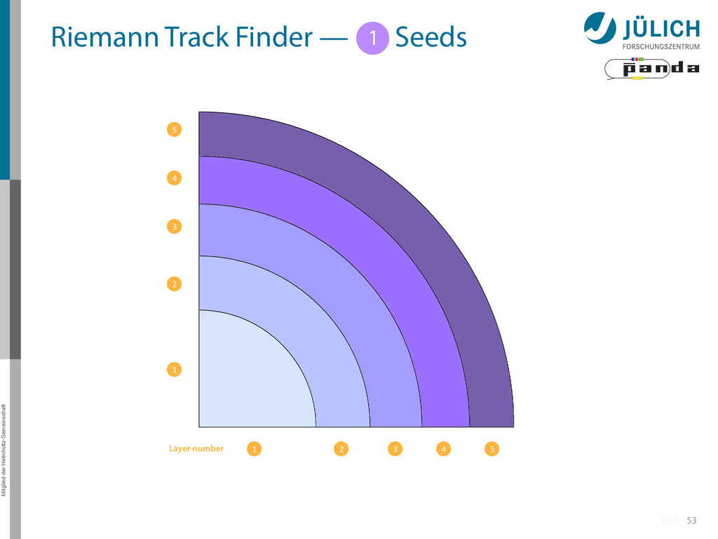
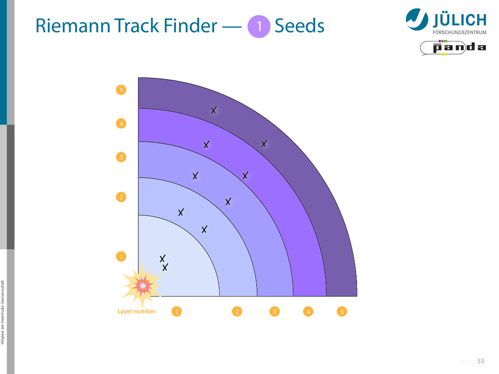
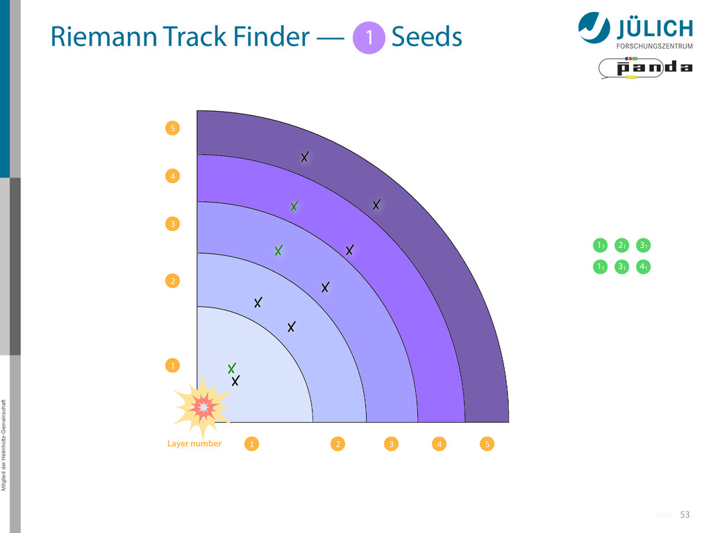
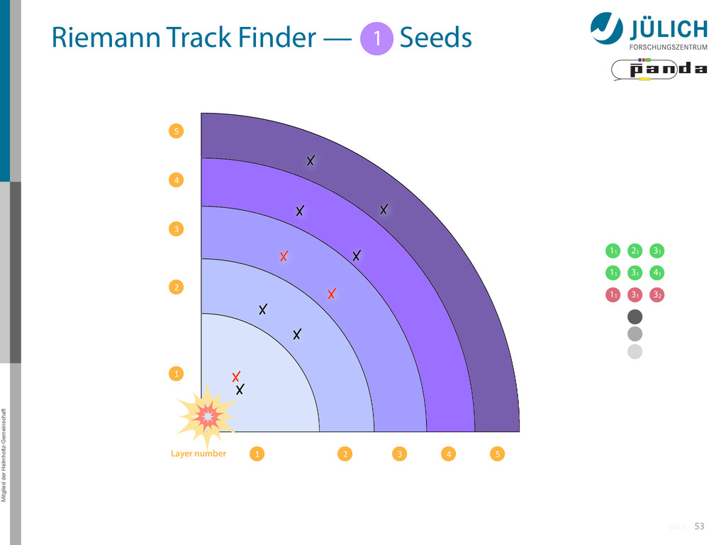
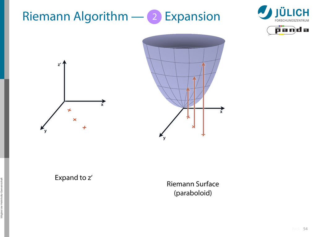
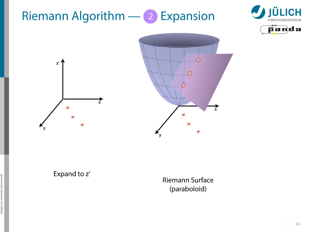
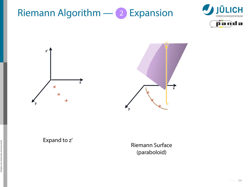
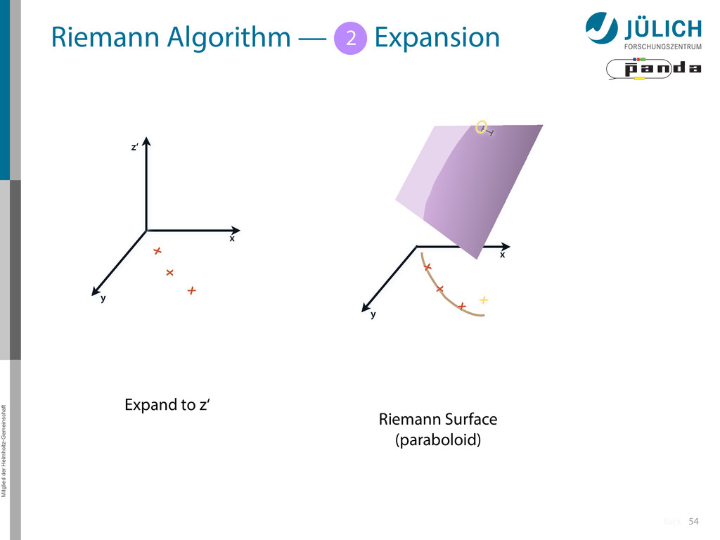
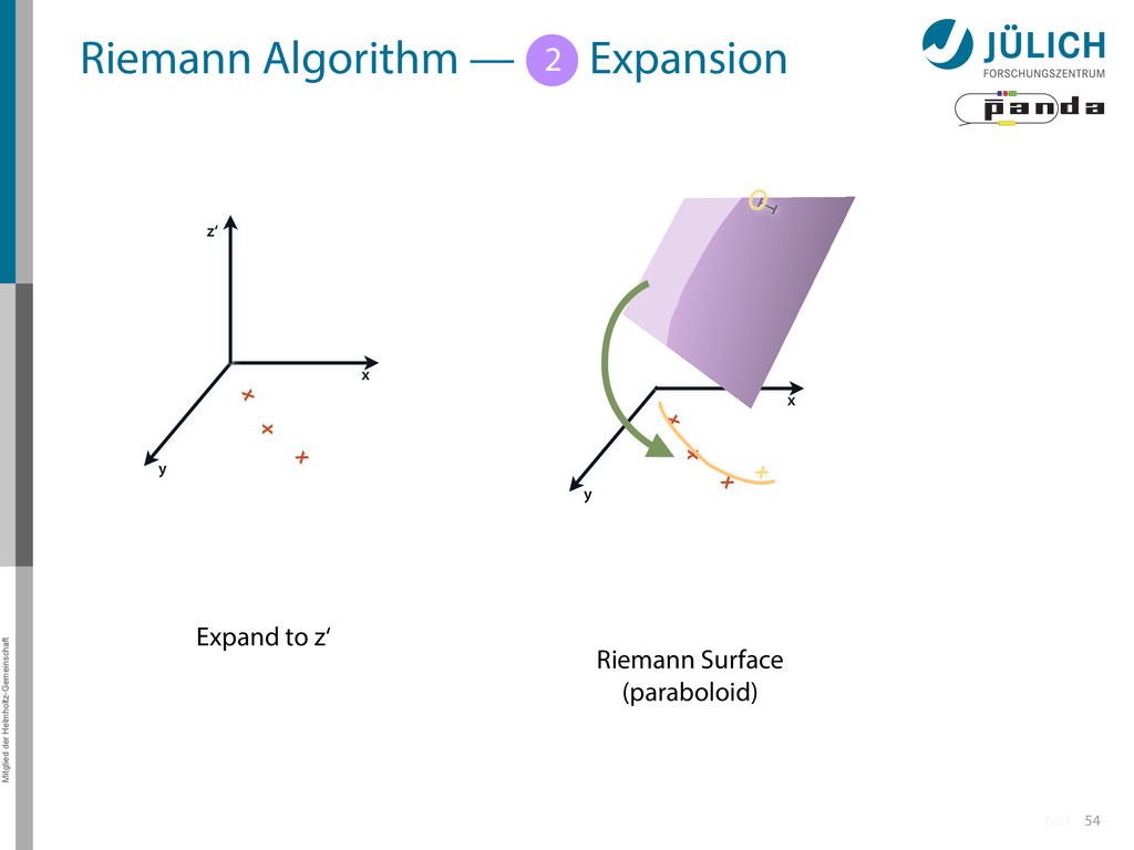
Idea: Don‘t fit lines (in 2D), fit planes (in 3D)! • Create seeds – All possible three hit combinations • Grow seeds to tracks Continuously test next hit if it fits – Use mapping to Riemann paraboloid (+ s-z fit, det. layer) x x x x y z‘ x x x y x x x x y x More on: Seeds; Growing 1 2
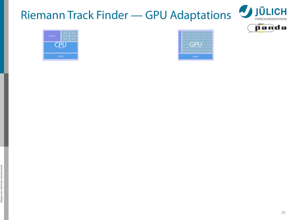
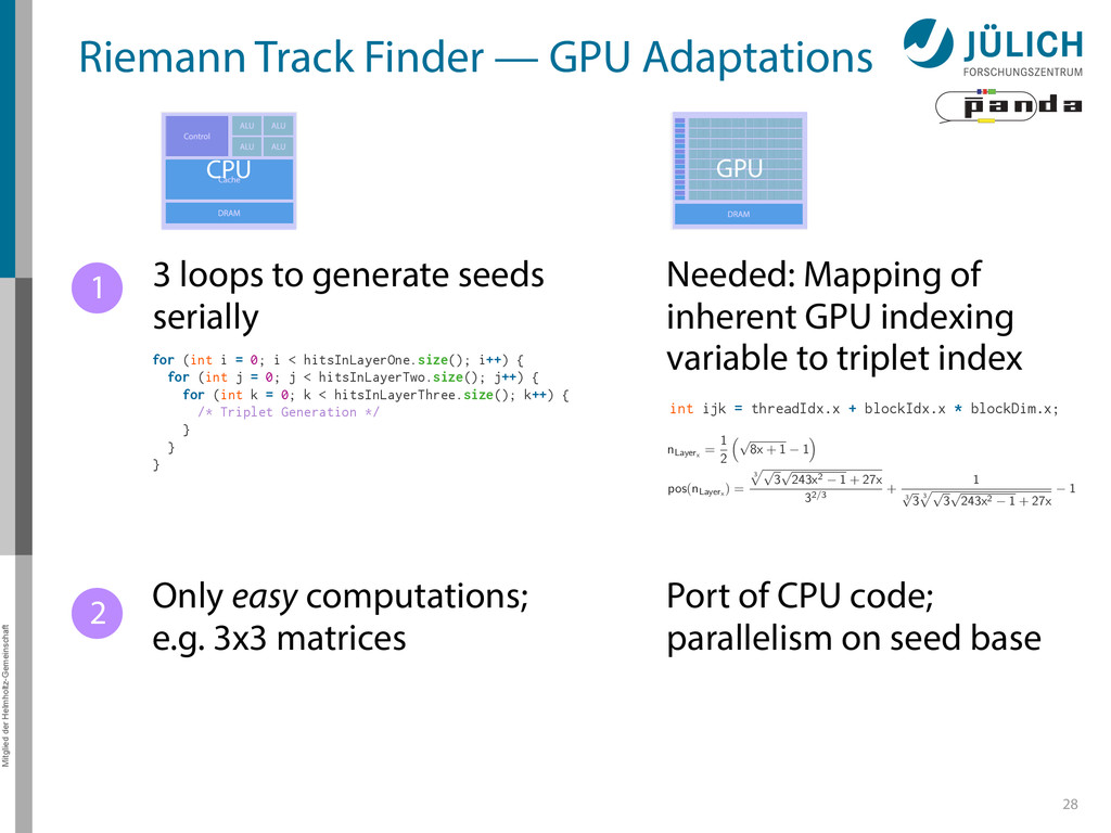
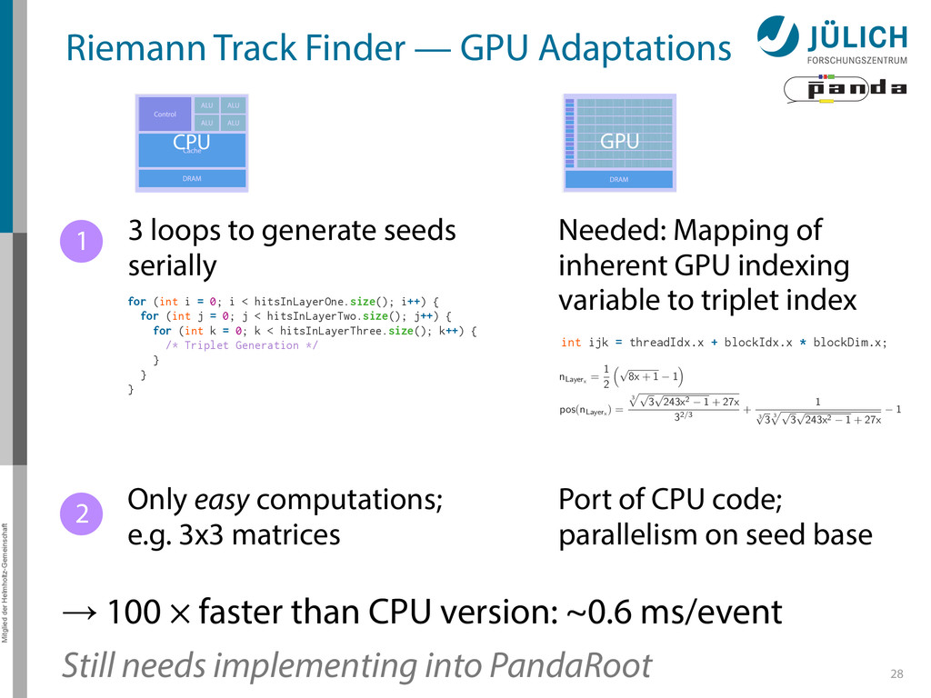
CPU GPU → 100 × faster than CPU version: ~0.6 ms/event Still needs implementing into PandaRoot 3 loops to generate seeds serially for (int i = 0; i < hitsInLayerOne.size(); i++) { for (int j = 0; j < hitsInLayerTwo.size(); j++) { for (int k = 0; k < hitsInLayerThree.size(); k++) { /* Triplet Generation */ } } } Needed: Mapping of inherent GPU indexing variable to triplet index int ijk = threadIdx.x + blockIdx.x * blockDim.x; nLayerx = 1 2 ⇣p 8x + 1 1 ⌘ pos ( nLayerx ) = 3 pp 3 p 243x2 1 + 27x 32 / 3 + 1 3 p 3 3 pp 3 p 243x2 1 + 27x 1 1 2 Port of CPU code; parallelism on seed base Only easy computations; e.g. 3x3 matrices
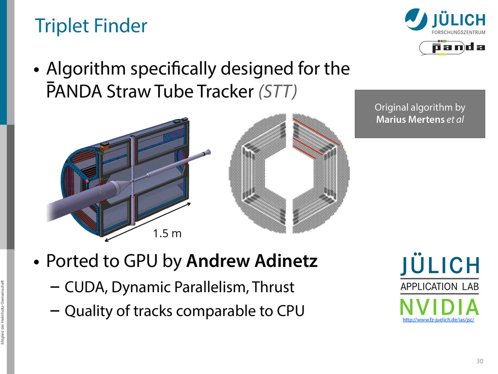
for the PANDA Straw Tube Tracker (STT) • Ported to GPU by Andrew Adinetz – CUDA, Dynamic Parallelism, Thrust – Quality of tracks comparable to CPU http://www.fz-juelich.de/ias/jsc/ Original algorithm by Marius Mertens et al 1.5 m
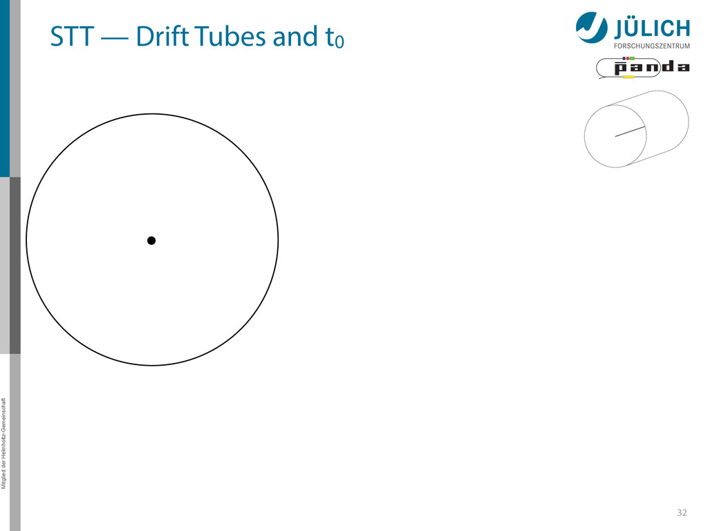
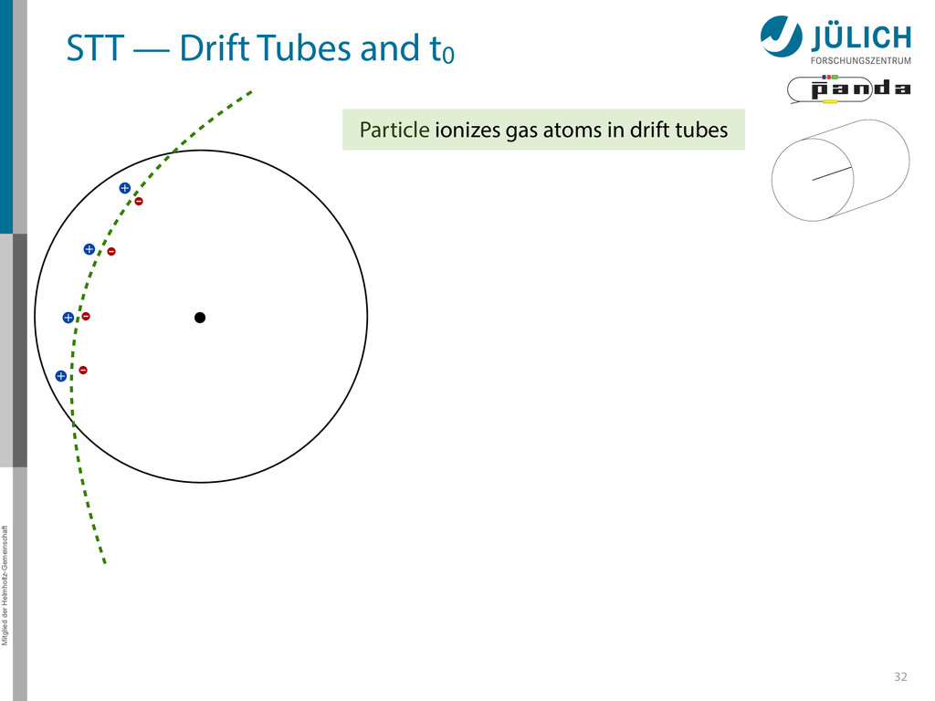
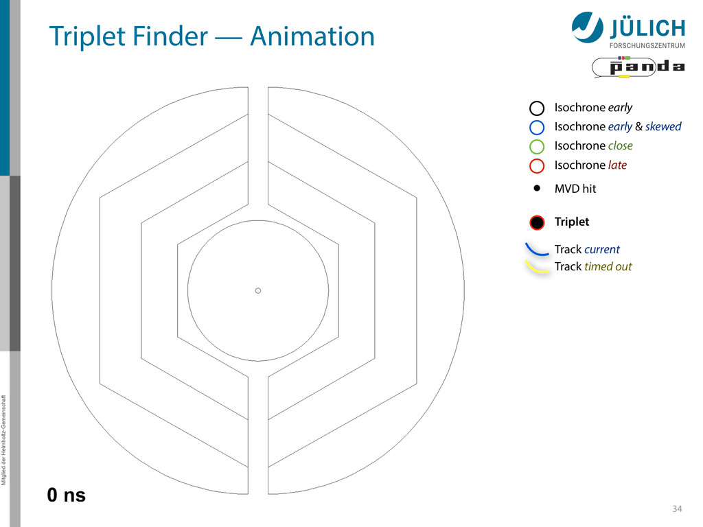
Particle ionizes gas atoms in drift tubes Electrons drift to anode wire, ions to wall Signal only when electrons arrive at wire No information about drift duration! For that, start time (t0) needed: t0 - tarrival ≈ tdrift vdrift = const → tdrift • vdrift = risochrone
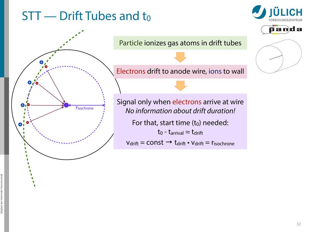
Particle ionizes gas atoms in drift tubes Electrons drift to anode wire, ions to wall Signal only when electrons arrive at wire No information about drift duration! For that, start time (t0) needed: t0 - tarrival ≈ tdrift vdrift = const → tdrift • vdrift = risochrone risochrone
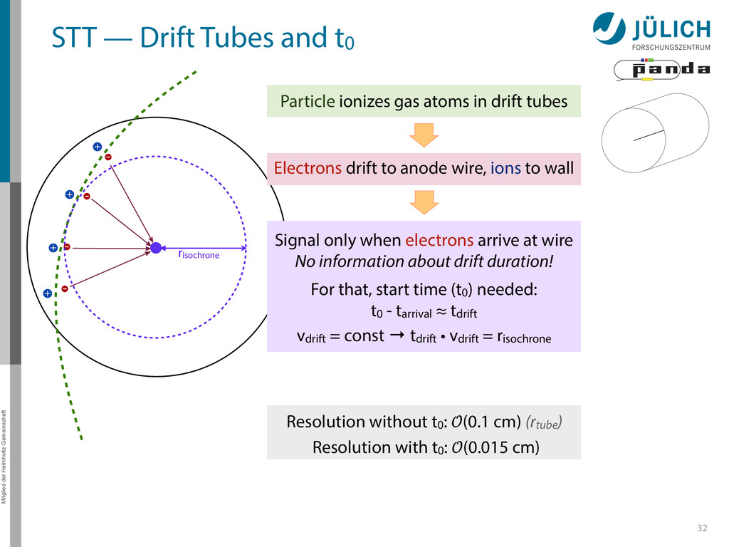
Particle ionizes gas atoms in drift tubes Resolution without t0: (0.1 cm) (rtube) Resolution with t0: (0.015 cm) Electrons drift to anode wire, ions to wall Signal only when electrons arrive at wire No information about drift duration! For that, start time (t0) needed: t0 - tarrival ≈ tdrift vdrift = const → tdrift • vdrift = risochrone risochrone
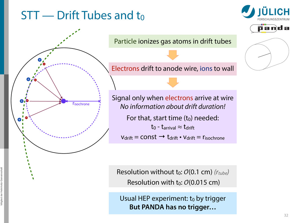
Particle ionizes gas atoms in drift tubes Resolution without t0: (0.1 cm) (rtube) Resolution with t0: (0.015 cm) Usual HEP experiment: t0 by trigger But PANDA has no trigger… Electrons drift to anode wire, ions to wall Signal only when electrons arrive at wire No information about drift duration! For that, start time (t0) needed: t0 - tarrival ≈ tdrift vdrift = const → tdrift • vdrift = risochrone risochrone
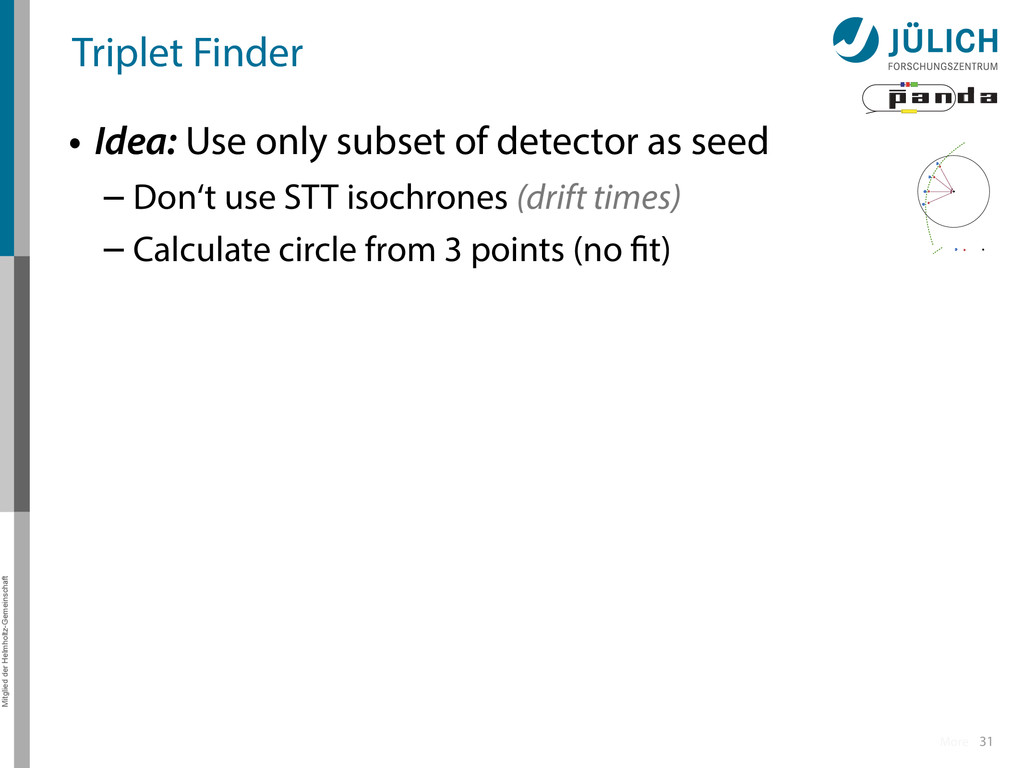
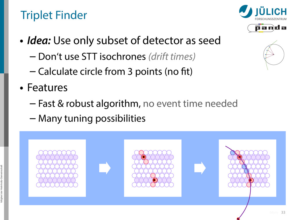
subset of detector as seed – Don‘t use STT isochrones (drift times) – Calculate circle from 3 points (no fit) • Features – Fast & robust algorithm, no event time needed – Many tuning possibilities More
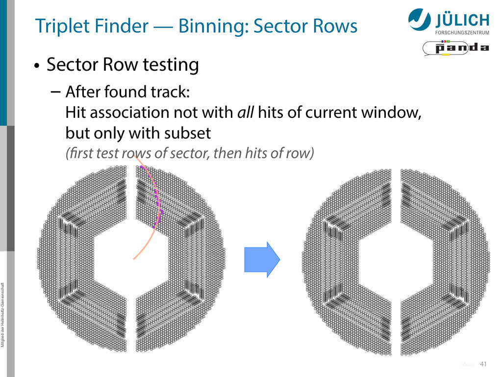
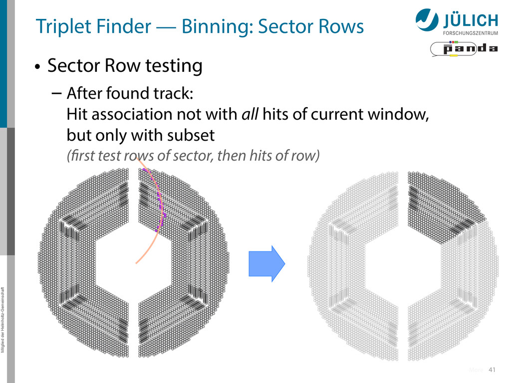
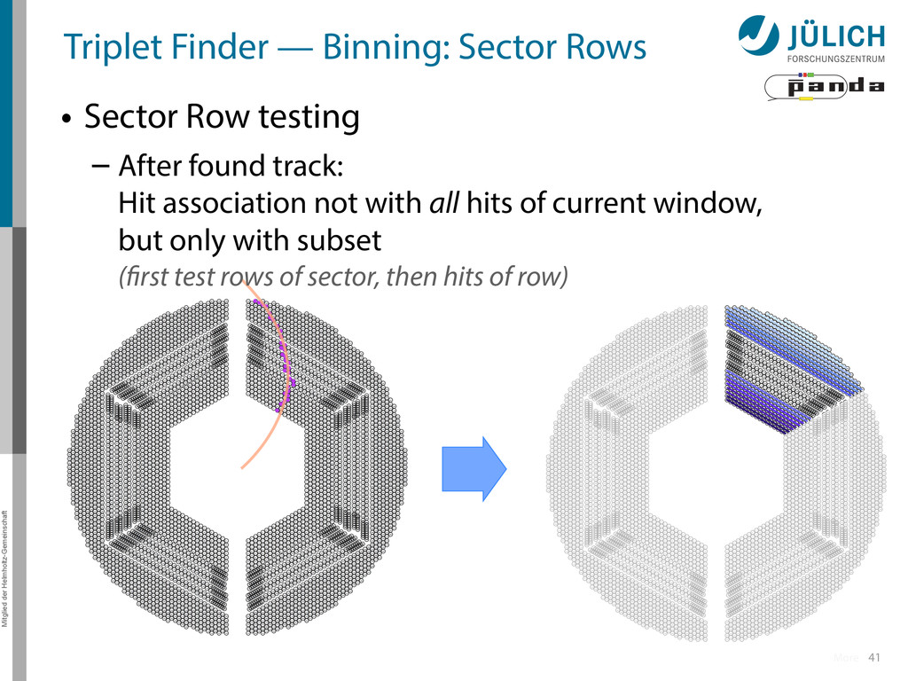
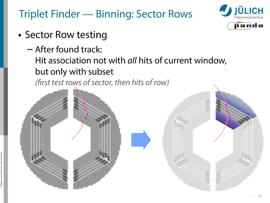
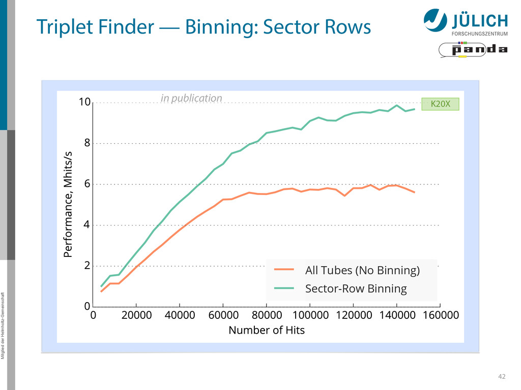
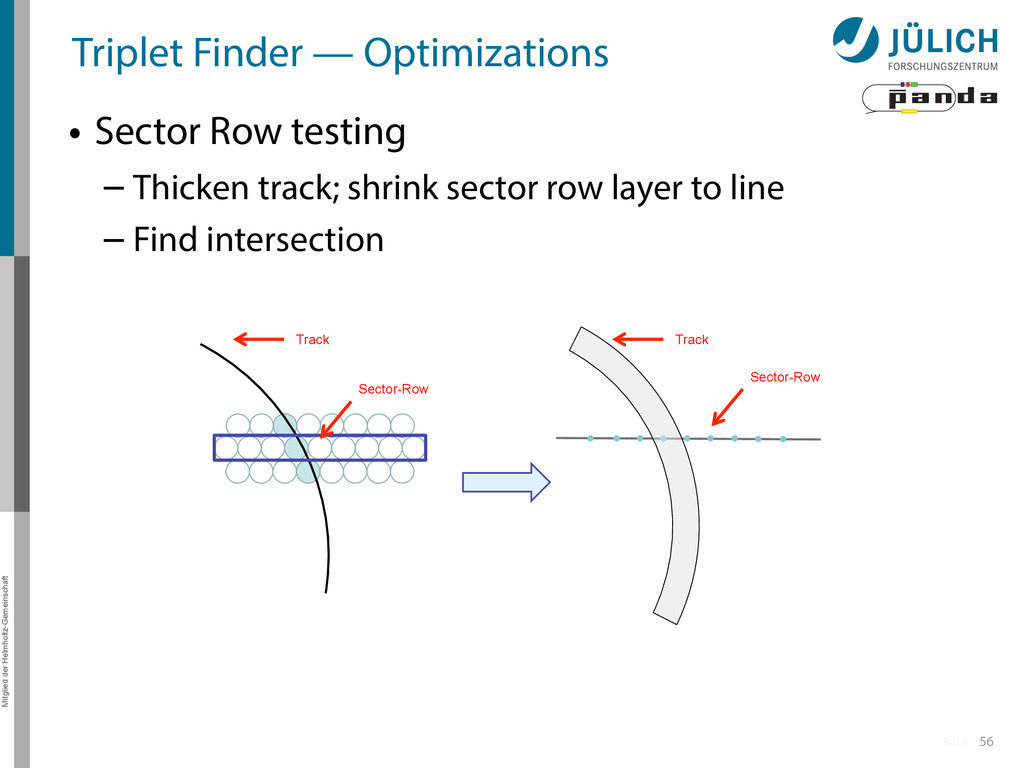
• Sector Row testing – After found track: Hit association not with all hits of current window, but only with subset (first test rows of sector, then hits of row) More
• Sector Row testing – After found track: Hit association not with all hits of current window, but only with subset (first test rows of sector, then hits of row) More
• Sector Row testing – After found track: Hit association not with all hits of current window, but only with subset (first test rows of sector, then hits of row) More
• Sector Row testing – After found track: Hit association not with all hits of current window, but only with subset (first test rows of sector, then hits of row) More
• Sector Row testing – After found track: Hit association not with all hits of current window, but only with subset (first test rows of sector, then hits of row) More
14 µs/event – 14⋅10-6 s/event * 2⋅107 event/s 㱺 280 GPUs2014 – PANDA2019: Multi GPU system – (100) GPUs • Optimizations possible & needed – ε needs to be improved – Speed, €: • More float less double-cards a la K10 • Consumer-grade cards a la GTX 47
as part of online event reconstruction scheme • Algorithms in active evaluation and optimization – Triplet Finder performance-optimized • Data transfer to GPU in research: FairMQ 48
PANDA researches in using GPUs as part of online event reconstruction scheme • Algorithms in active evaluation and optimization – Triplet Finder performance-optimized • Data transfer to GPU in research: FairMQ 48
icon by Nikki Rodriguez from The Noun Project • #3: Einstein icon by Roman Rusinov from The Noun Project • #6: FAIR vector logo from official FAIR website • #6: FAIR rendering from official website • #11: Flare Gun icon by Jop van der Kroef from The Noun Project • #27: STT event animation by Marius C. Mertens • #35: Graphics cards images by NVIDIA promotion • #35: GPU Specifications – Tesla K20X Specifications: http://www.nvidia.com/content/PDF/kepler/Tesla- K20X-BD-06397-001-v07.pdf – Tesla K40 Specifications: http://www.nvidia.com/content/PDF/kepler/Tesla-K40- Active-Board-Spec-BD-06949-001_v03.pdf – Tesla Familiy Overview: http://www.nvidia.com/content/tesla/pdf/NVIDIA-Tesla- Kepler-Family-Datasheet.pdf 49
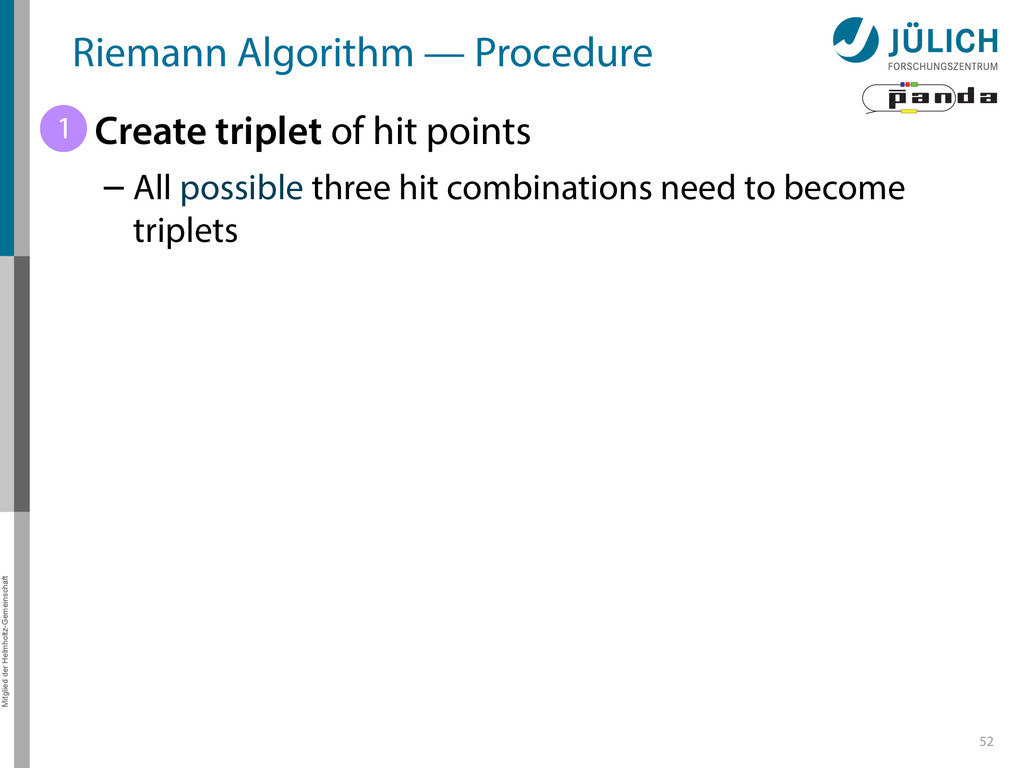
triplet of hit points – All possible three hit combinations need to become triplets • Grow triplets to tracks: Continuously test next hit if it fits to triplet track – Use Riemann paraboloid to circle fit track • Test closeness of new hit: good → add hit; bad → dismiss hit • Continue with next hit – Helix fit: arc length s vs. z position 1 2
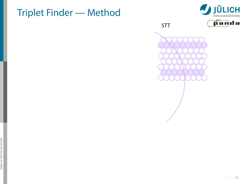
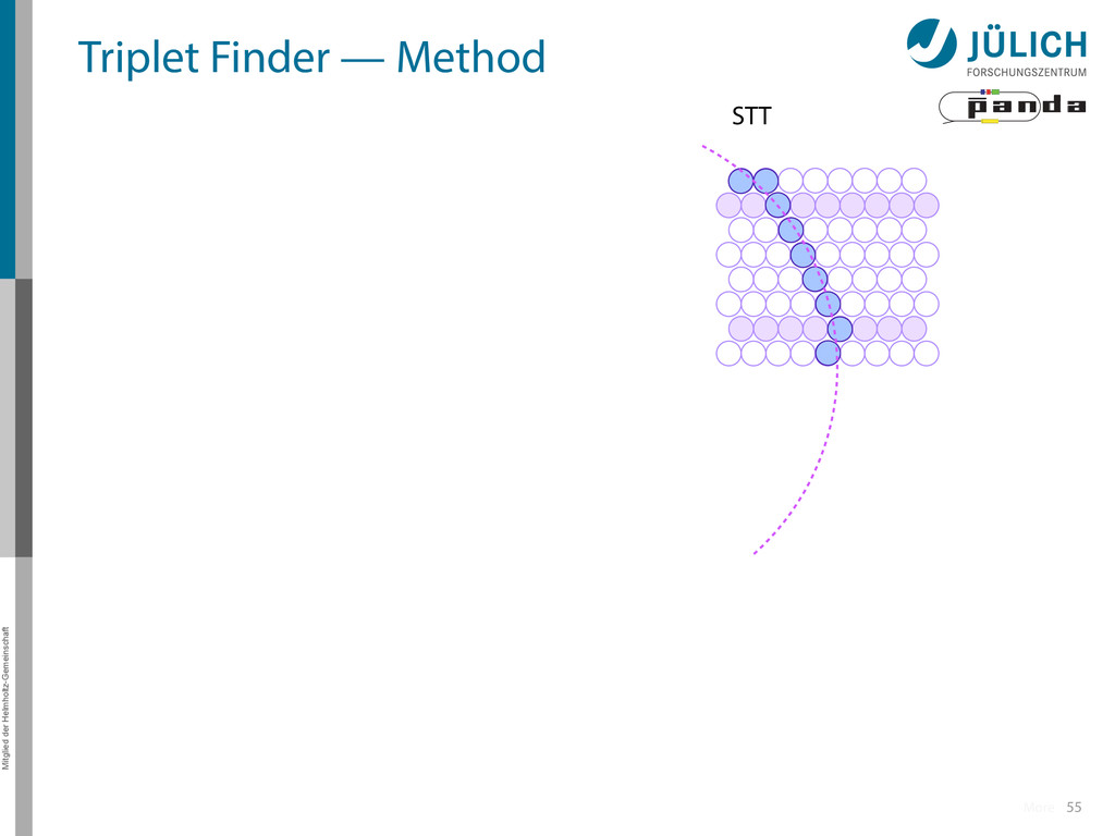
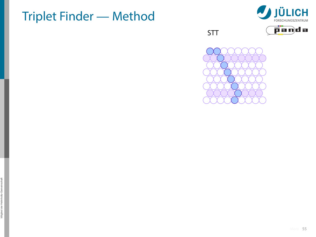
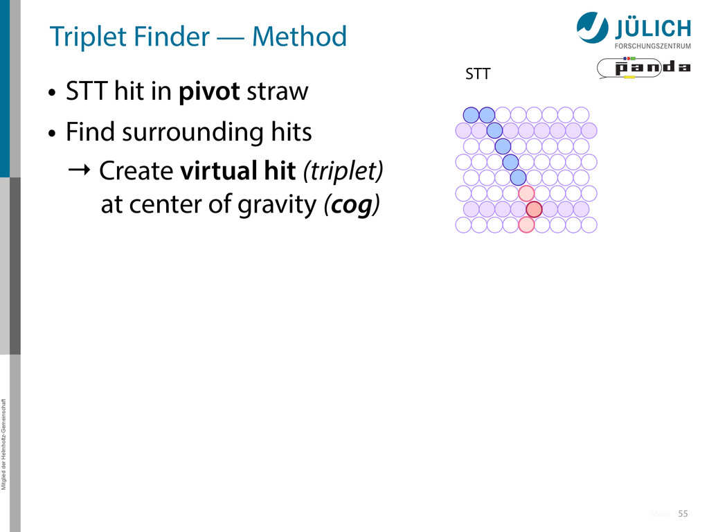
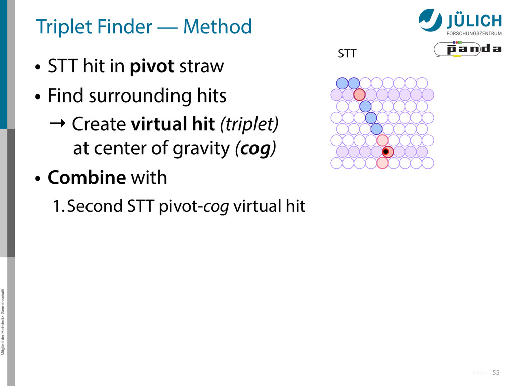
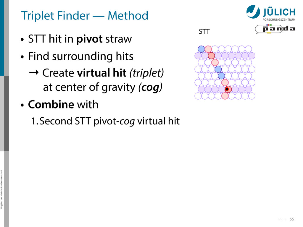
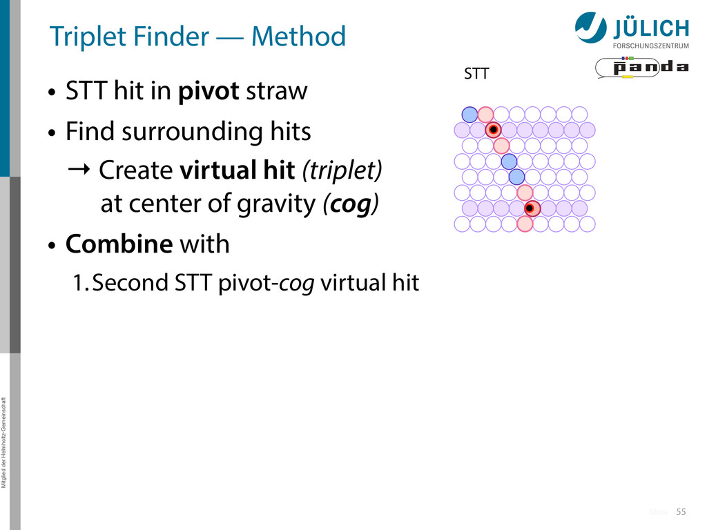
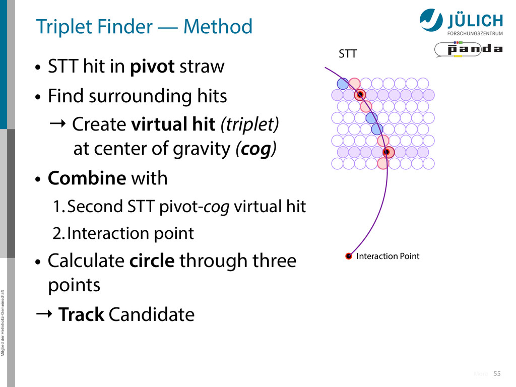
in pivot straw • Find surrounding hits → Create virtual hit (triplet) at center of gravity (cog) • Combine with 1.Second STT pivot-cog virtual hit 55 STT More
in pivot straw • Find surrounding hits → Create virtual hit (triplet) at center of gravity (cog) • Combine with 1.Second STT pivot-cog virtual hit 55 STT More
in pivot straw • Find surrounding hits → Create virtual hit (triplet) at center of gravity (cog) • Combine with 1.Second STT pivot-cog virtual hit 55 STT More
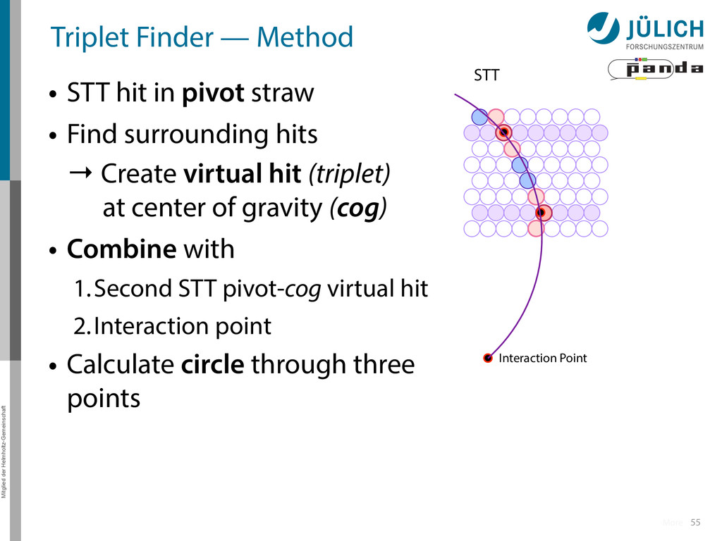
in pivot straw • Find surrounding hits → Create virtual hit (triplet) at center of gravity (cog) • Combine with 1.Second STT pivot-cog virtual hit 2.Interaction point 55 Interaction Point STT More
in pivot straw • Find surrounding hits → Create virtual hit (triplet) at center of gravity (cog) • Combine with 1.Second STT pivot-cog virtual hit 2.Interaction point • Calculate circle through three points 55 Interaction Point STT More
in pivot straw • Find surrounding hits → Create virtual hit (triplet) at center of gravity (cog) • Combine with 1.Second STT pivot-cog virtual hit 2.Interaction point • Calculate circle through three points → Track Candidate 55 Interaction Point STT More
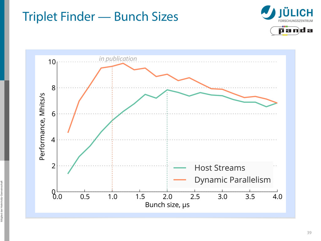
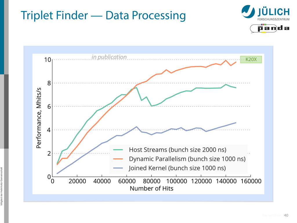
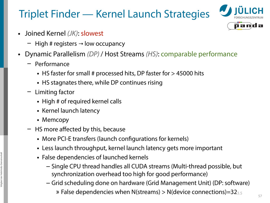
Joined Kernel (JK): slowest – High # registers → low occupancy • Dynamic Parallelism (DP) / Host Streams (HS): comparable performance – Performance • HS faster for small # processed hits, DP faster for > 45000 hits • HS stagnates there, while DP continues rising – Limiting factor • High # of required kernel calls • Kernel launch latency • Memcopy – HS more affected by this, because • More PCI-E transfers (launch configurations for kernels) • Less launch throughput, kernel launch latency gets more important • False dependencies of launched kernels – Single CPU thread handles all CUDA streams (Multi-thread possible, but synchronization overhead too high for good performance) – Grid scheduling done on hardware (Grid Management Unit) (DP: software) » False dependencies when N(streams) > N(device connections)=323.5 57 Back
![Thank you! Andreas Herten [email protected] Mitglied der Helmholtz-Gemeinschaft Summary •](https://files.speakerdeck.com/presentations/70b51dc0382701322c8976e1a203b64c/slide_142.jpg)