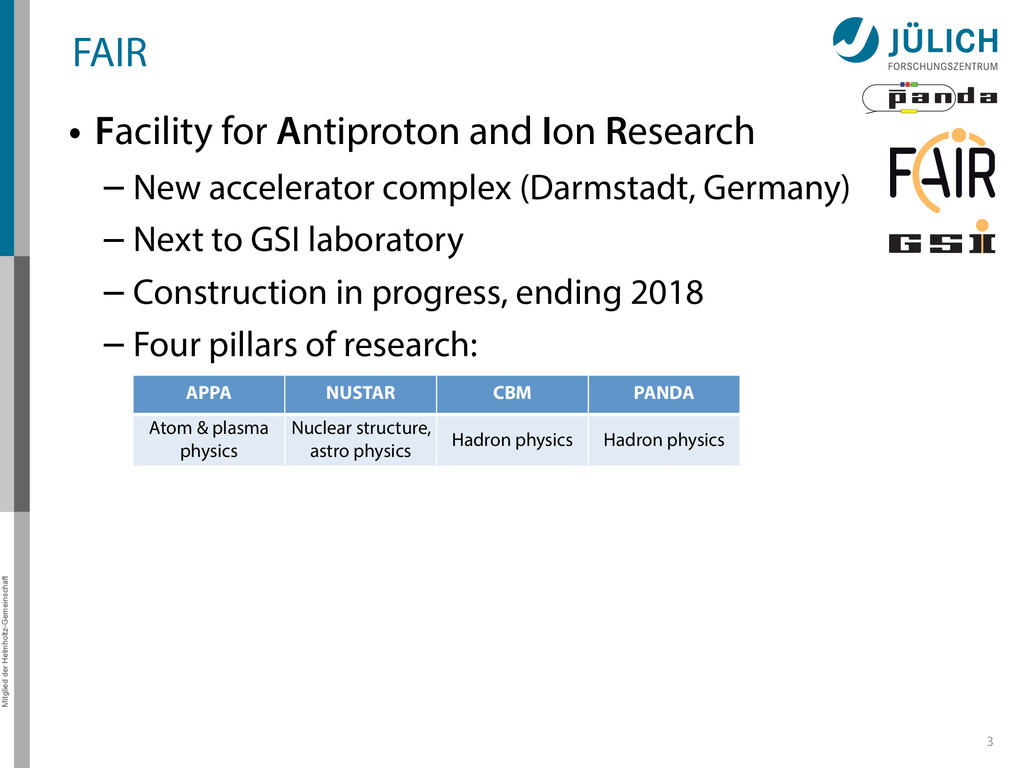
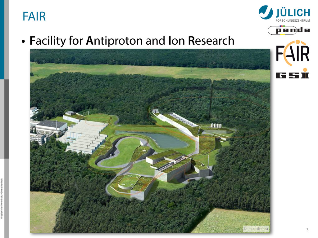
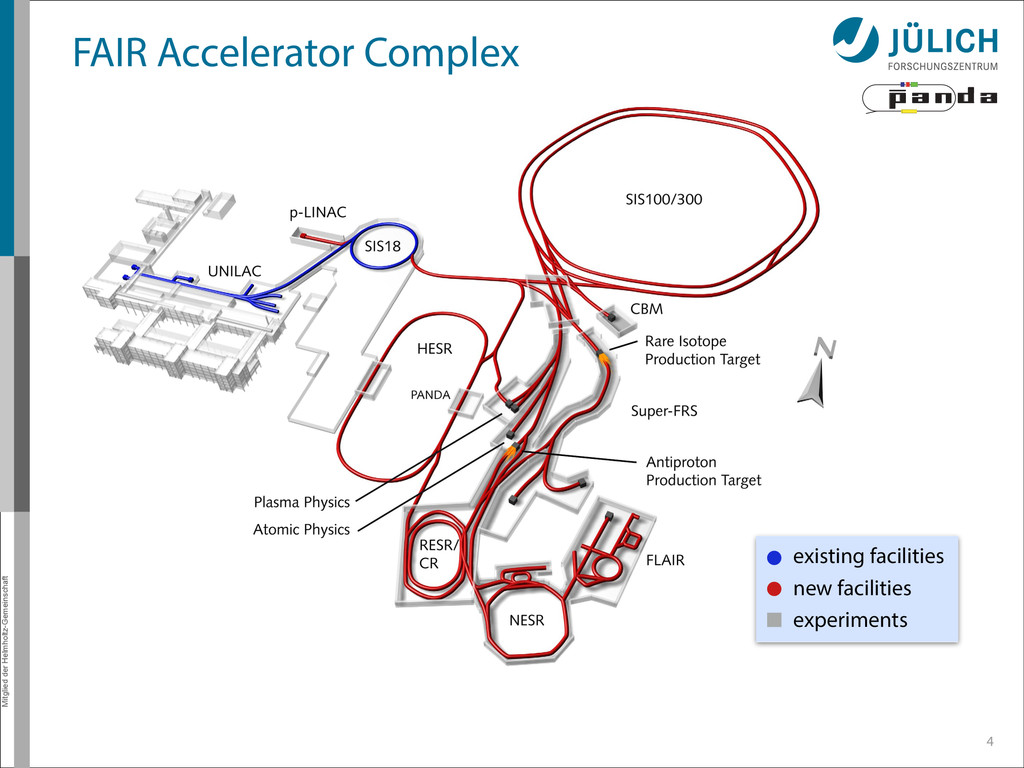
Research – New accelerator complex (Darmstadt, Germany) – Next to GSI laboratory – Construction in progress, ending 2018 – Four pillars of research: 3 APPA NUSTAR CBM PANDA Atom & plasma physics Nuclear structure, astro physics Hadron physics Hadron physics
Research – New accelerator complex (Darmstadt, Germany) – Next to GSI laboratory – Construction in progress, ending 2018 – Four pillars of research: 3 APPA NUSTAR CBM PANDA Atom & plasma physics Nuclear structure, astro physics Hadron physics Hadron physics
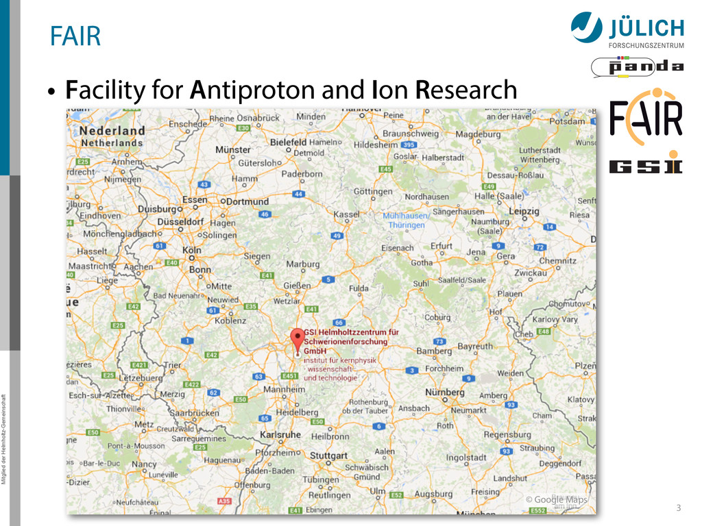
Research – New accelerator complex (Darmstadt, Germany) – Next to GSI laboratory – Construction in progress, ending 2018 – Four pillars of research: 3 APPA NUSTAR CBM PANDA Atom & plasma physics Nuclear structure, astro physics Hadron physics Hadron physics fair-center.eu
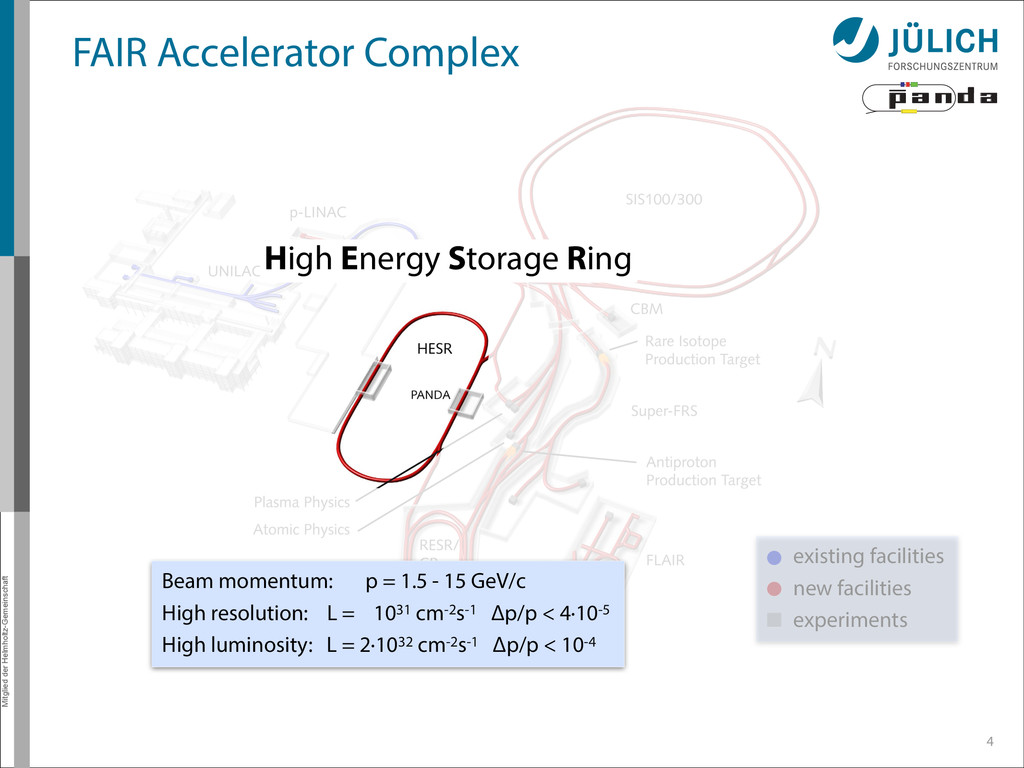
existing facilities new facilities experiments Beam momentum: p = 1.5 - 15 GeV/c High resolution: L = 1031 cm-2s-1 Δp/p < 4·10-5 High luminosity: L = 2·1032 cm-2s-1 Δp/p < 10-4 High Energy Storage Ring
Light mesons – Charmonium – Exotic states • Glueballs • Hybrids • Molecules/multiquarks – Open charm • Baryon production • Nucleon structure, e.m. processes • Charm in nuclei • Strangeness physics 7 0 2 4 6 8 12 15 10 p Momentum / GeV/c Mass / GeV/c2 1 2 3 4 5 6 ΛΛ ΣΣ ΞΞ Λ c Λ c Σ c Σ c Ξ c Ξ c Ω c Ω c ΩΩ DD D s D s ggg,gg light qq π,ρ,ω,f 2 ,K,K* cc J/ψ, η c , χ cJ qqqq ccqq nng,ssg ccg nng,ssg ccg ggg
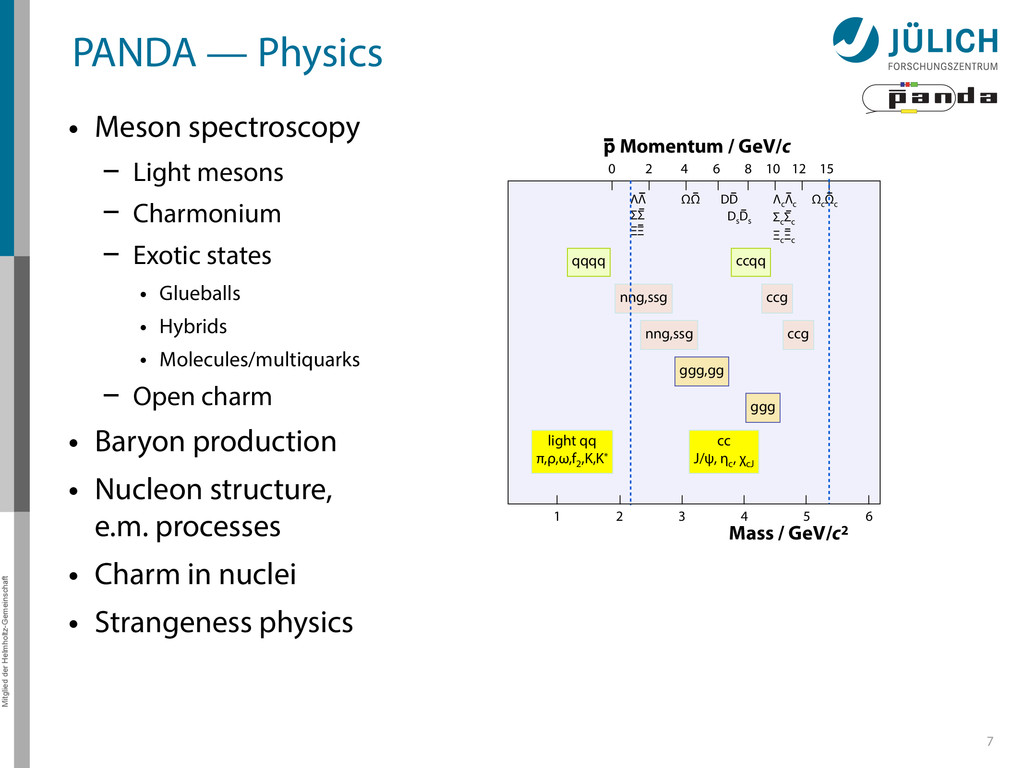
Light mesons – Charmonium – Exotic states • Glueballs • Hybrids • Molecules/multiquarks – Open charm • Baryon production • Nucleon structure, e.m. processes • Charm in nuclei • Strangeness physics 7 → Broad physics program 0 2 4 6 8 12 15 10 p Momentum / GeV/c Mass / GeV/c2 1 2 3 4 5 6 ΛΛ ΣΣ ΞΞ Λ c Λ c Σ c Σ c Ξ c Ξ c Ω c Ω c ΩΩ DD D s D s ggg,gg light qq π,ρ,ω,f 2 ,K,K* cc J/ψ, η c , χ cJ qqqq ccqq nng,ssg ccg nng,ssg ccg ggg
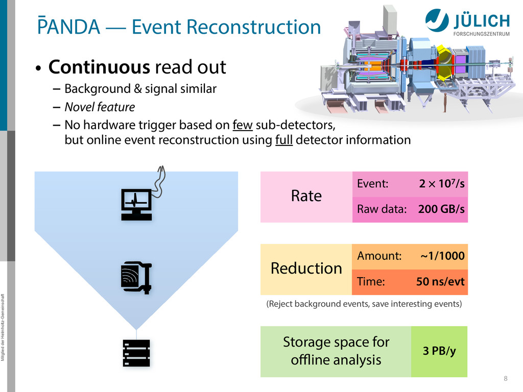
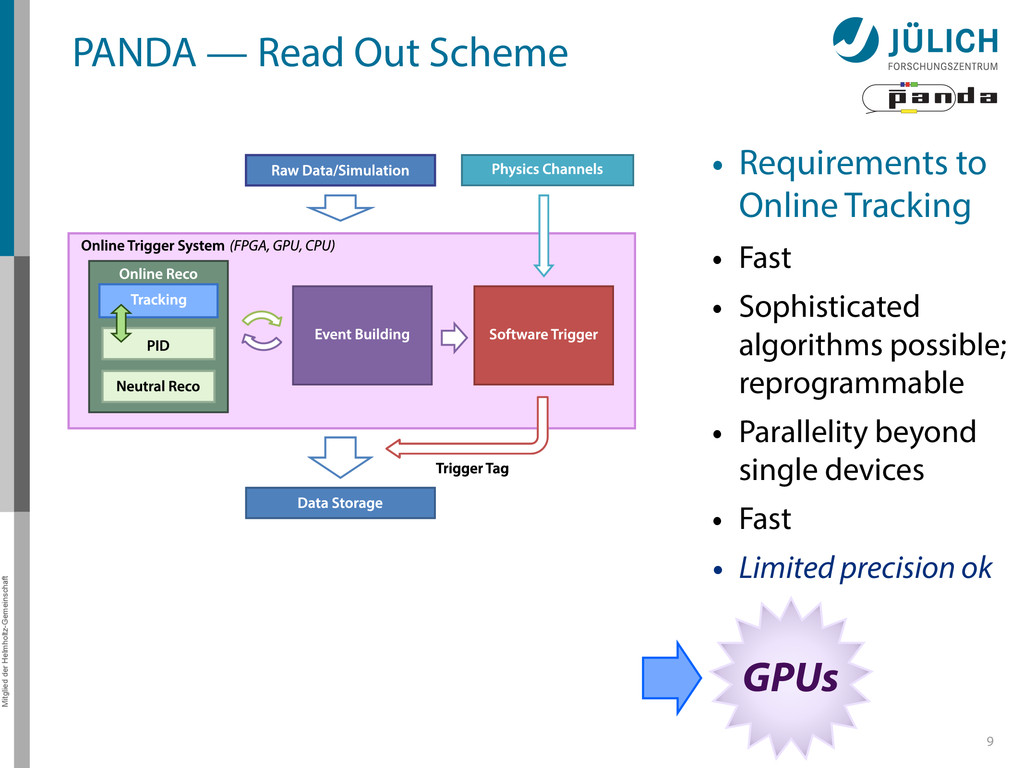
out – Background & signal similar – Novel feature – No hardware trigger based on few sub-detectors, but online event reconstruction using full detector information 8 (Reject background events, save interesting events) Reduction Amount: Time: ~1/1000 50 ns/evt Storage space for offline analysis 3 PB/y Event: Raw data: 2 × 10⁷/s 200 GB/s Rate
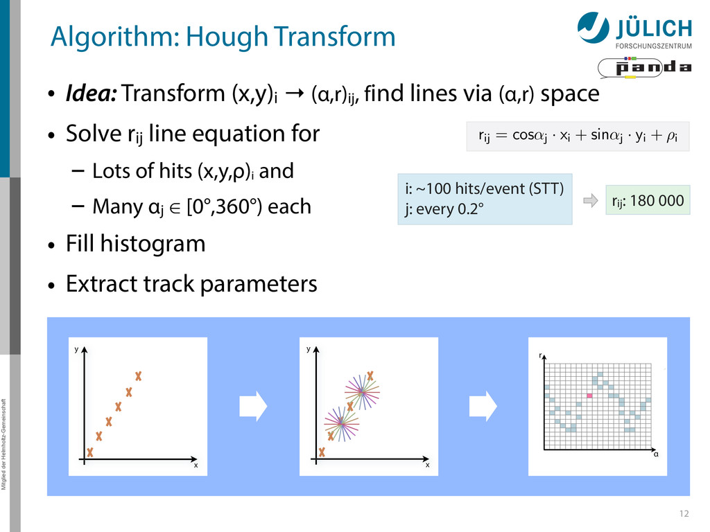
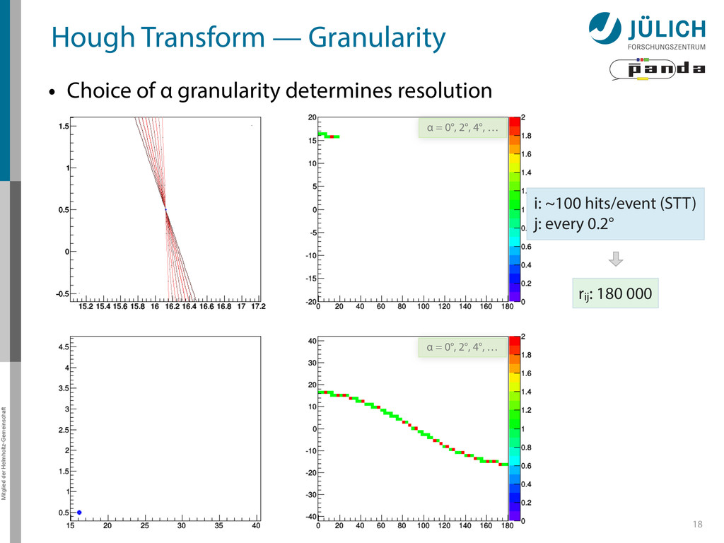
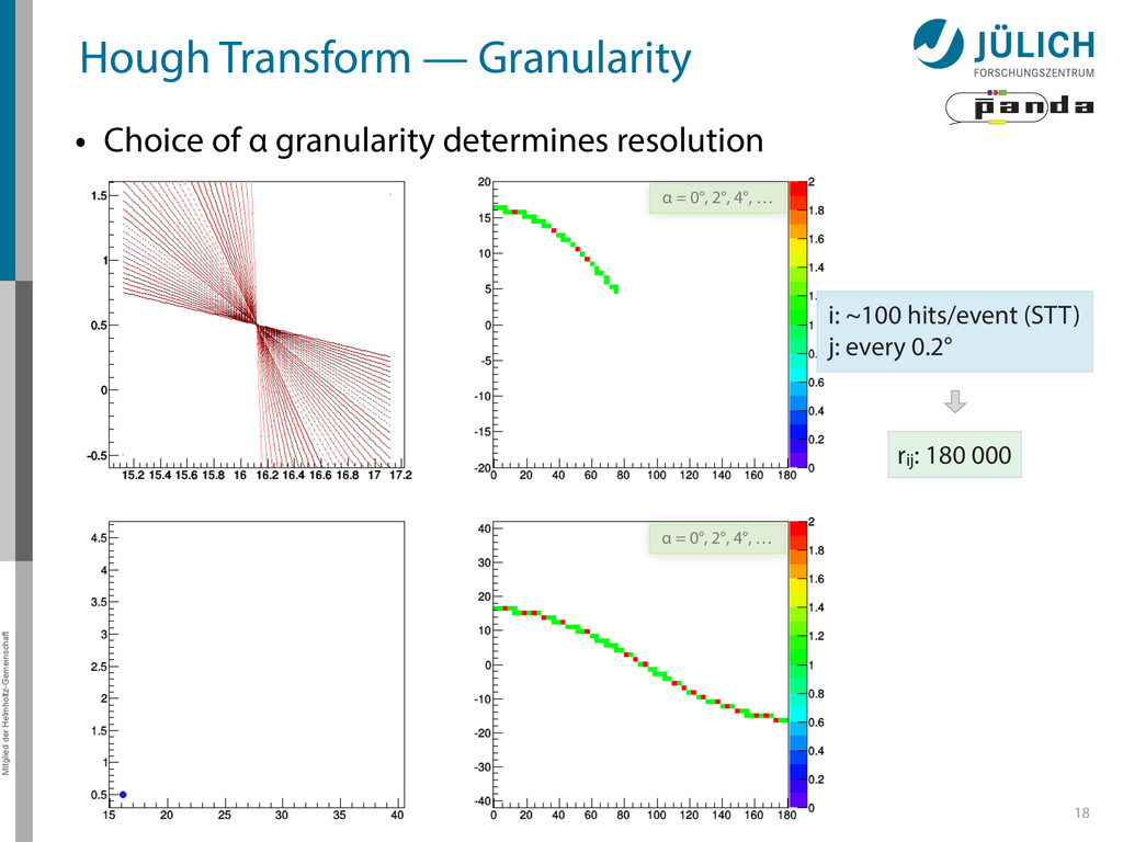
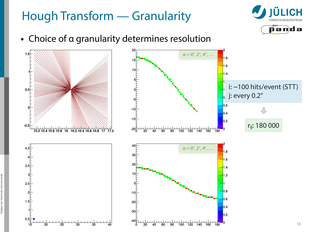
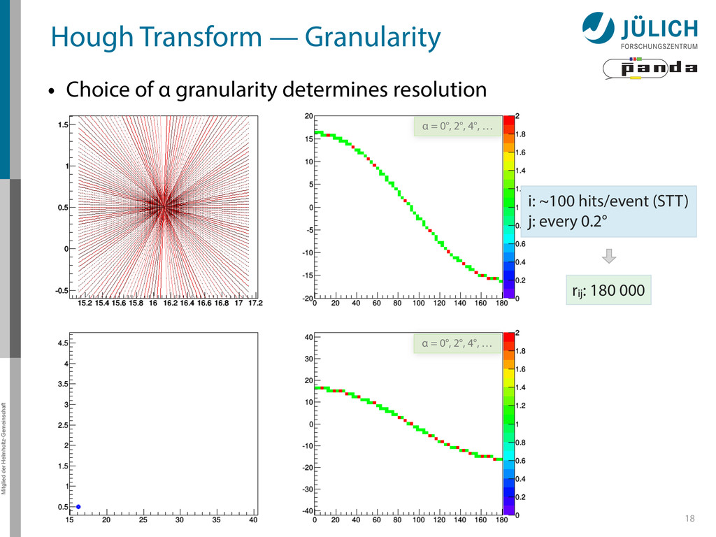
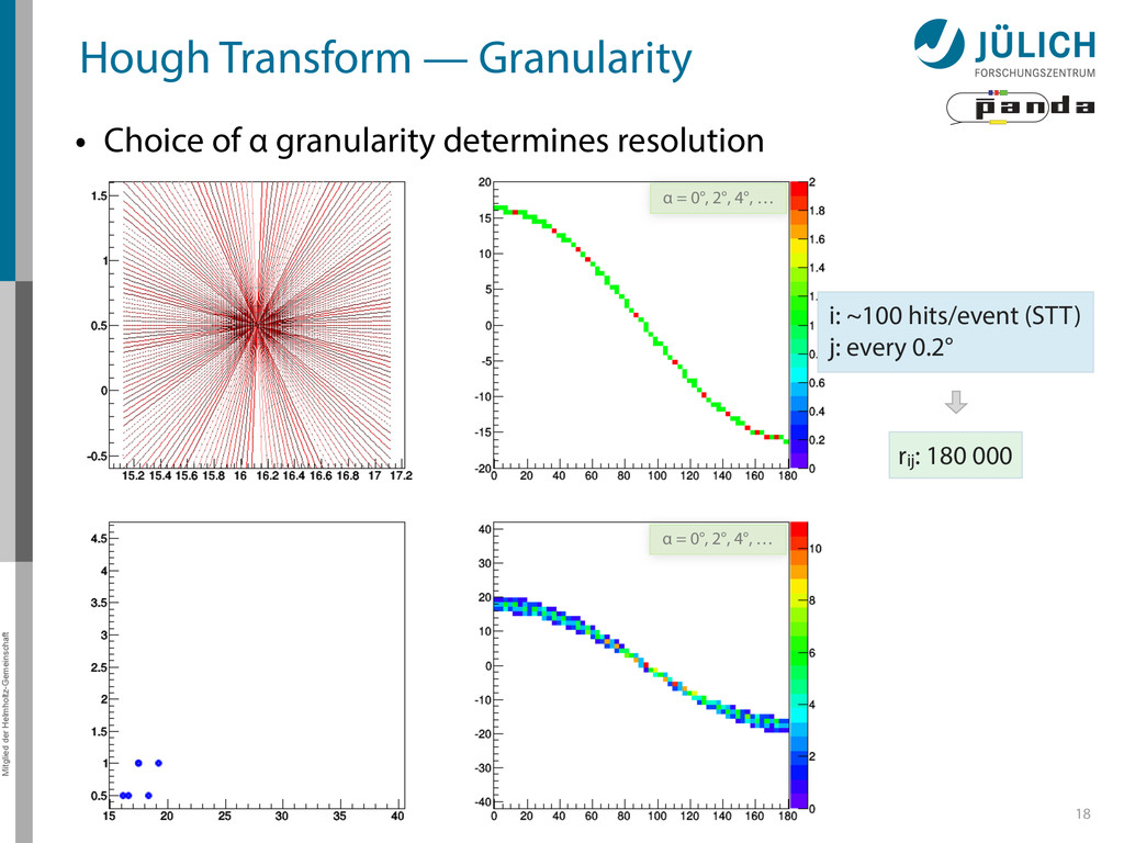
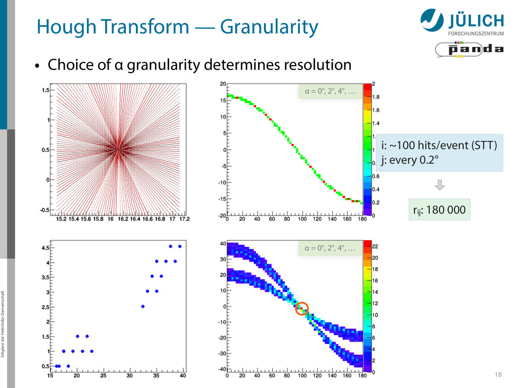
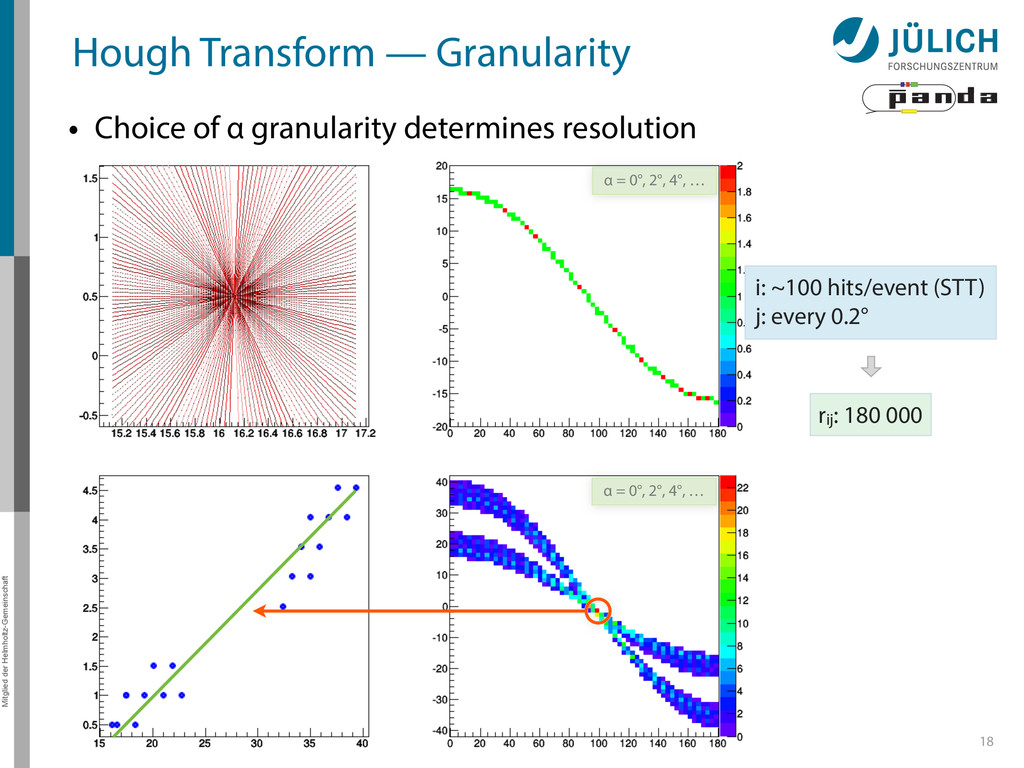
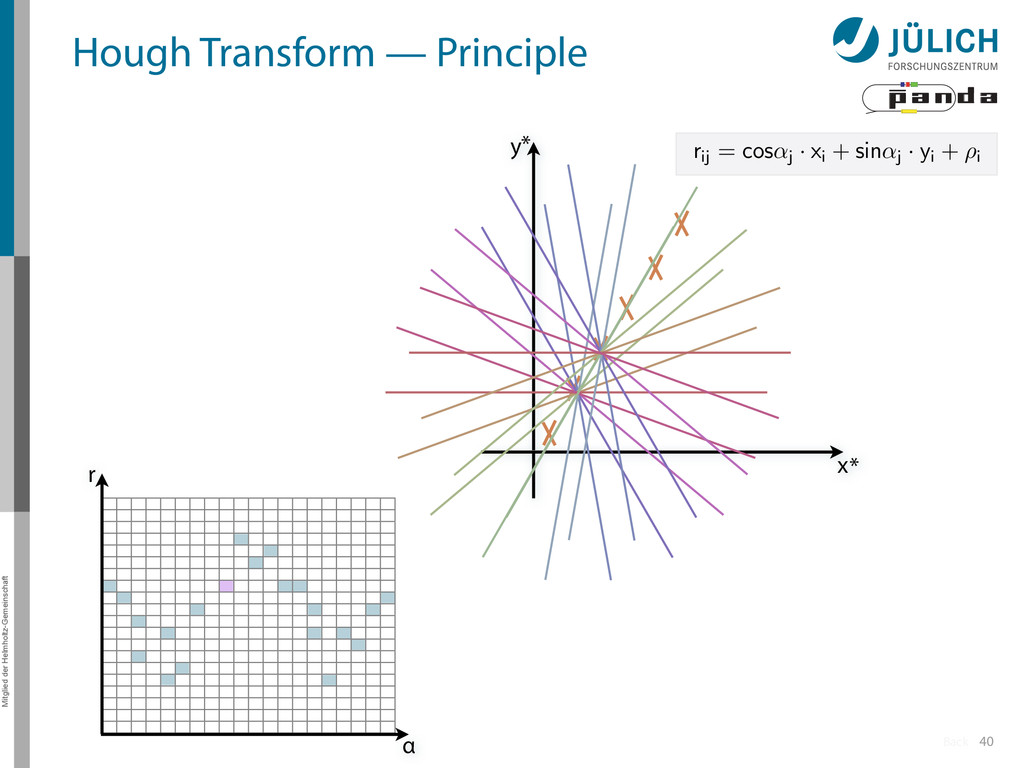
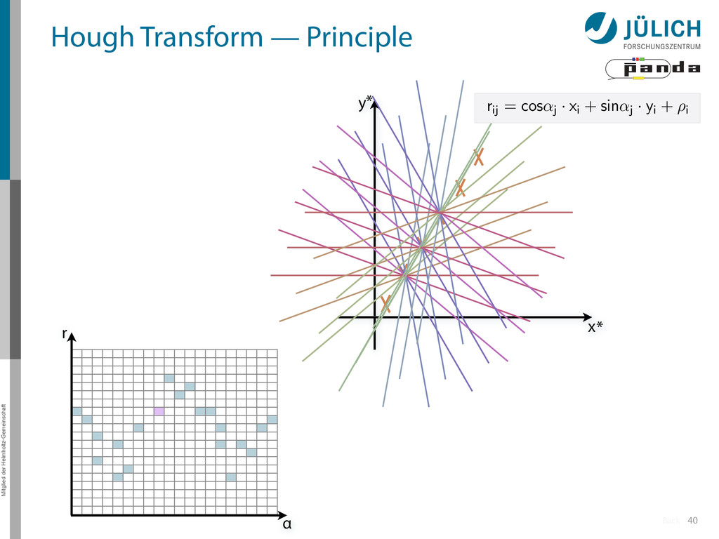
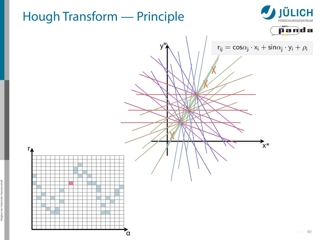
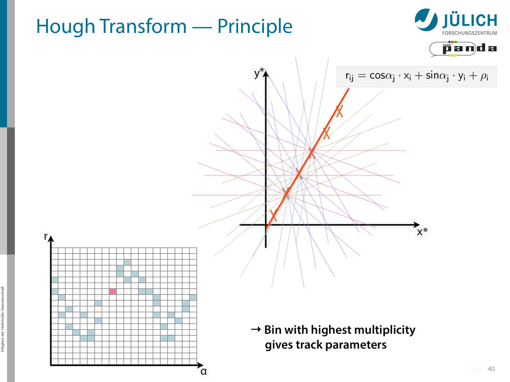
→ (α,r)ij , find lines via (α,r) space • Solve rij line equation for – Lots of hits (x,y,ρ)i and – Many αj ∈ [0°,360°) each • Fill histogram • Extract track parameters 12 rij = cos ↵j · xi + sin ↵j · yi + ⇢i i: ~100 hits/event (STT) j: every 0.2° rij : 180 000 x y x y Mitglied der Helmholtz-Gemeinschaft Hough Transform — Princip → Bin giv r α
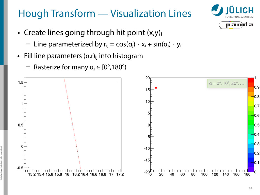
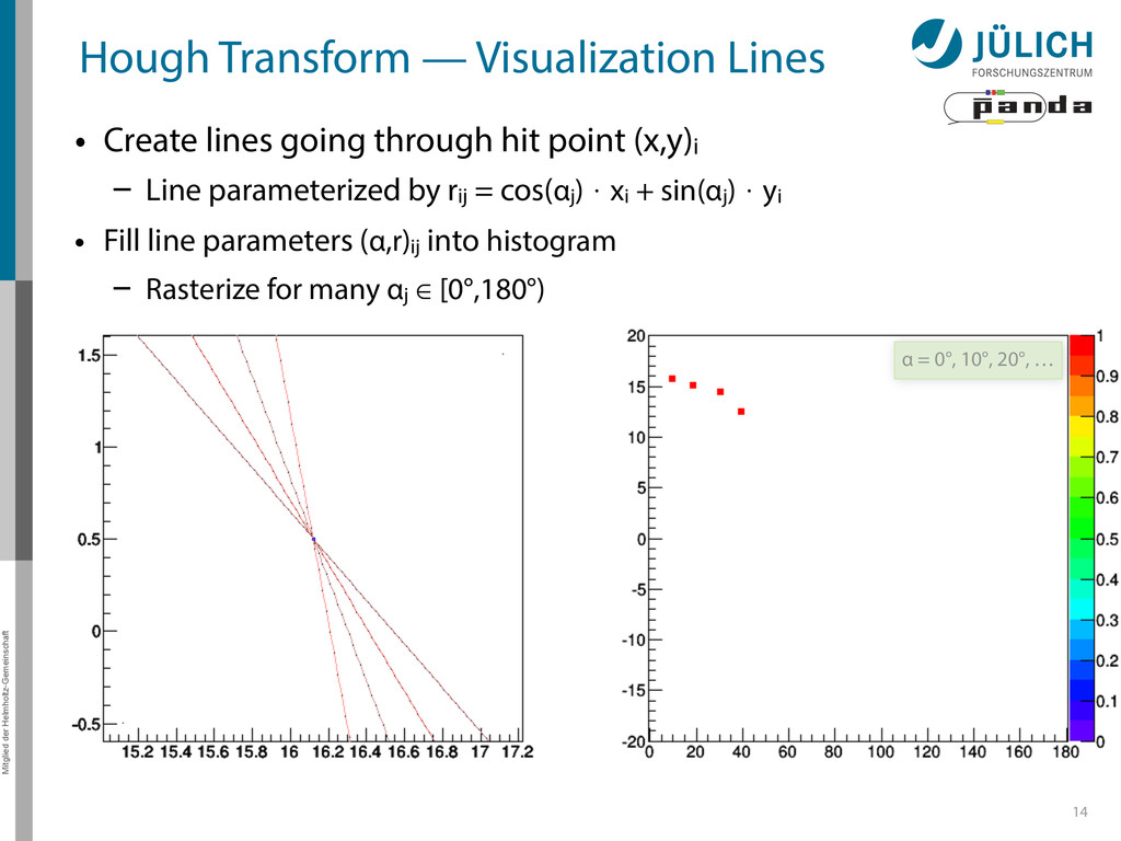
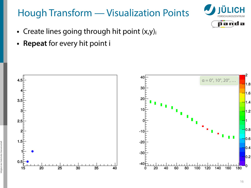
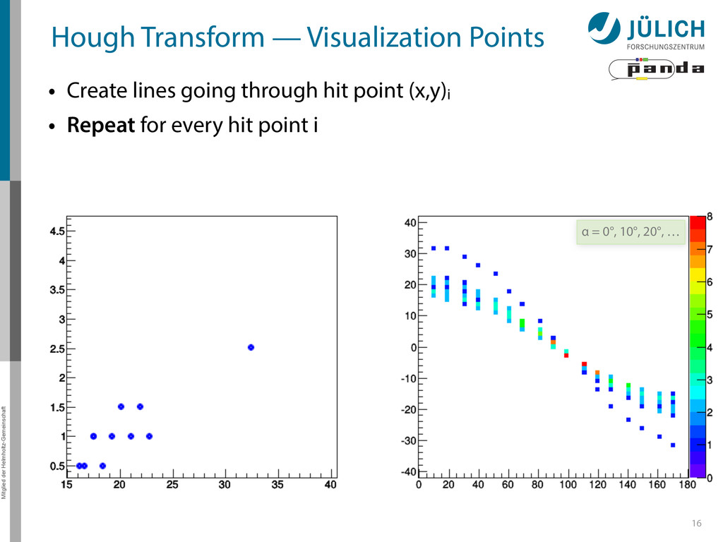
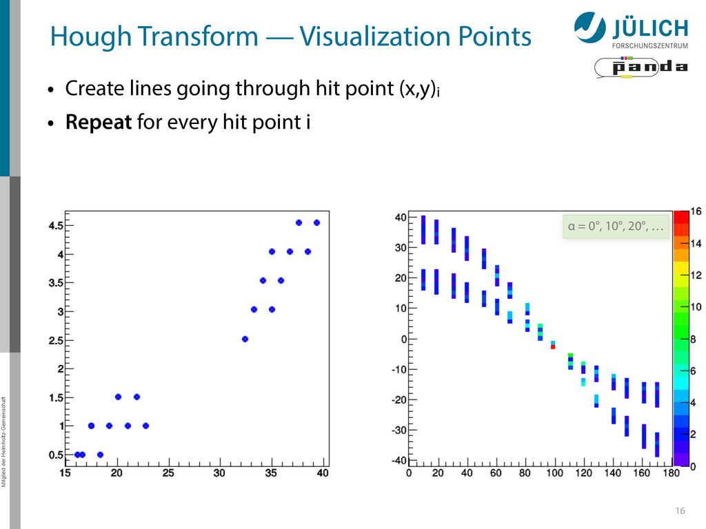
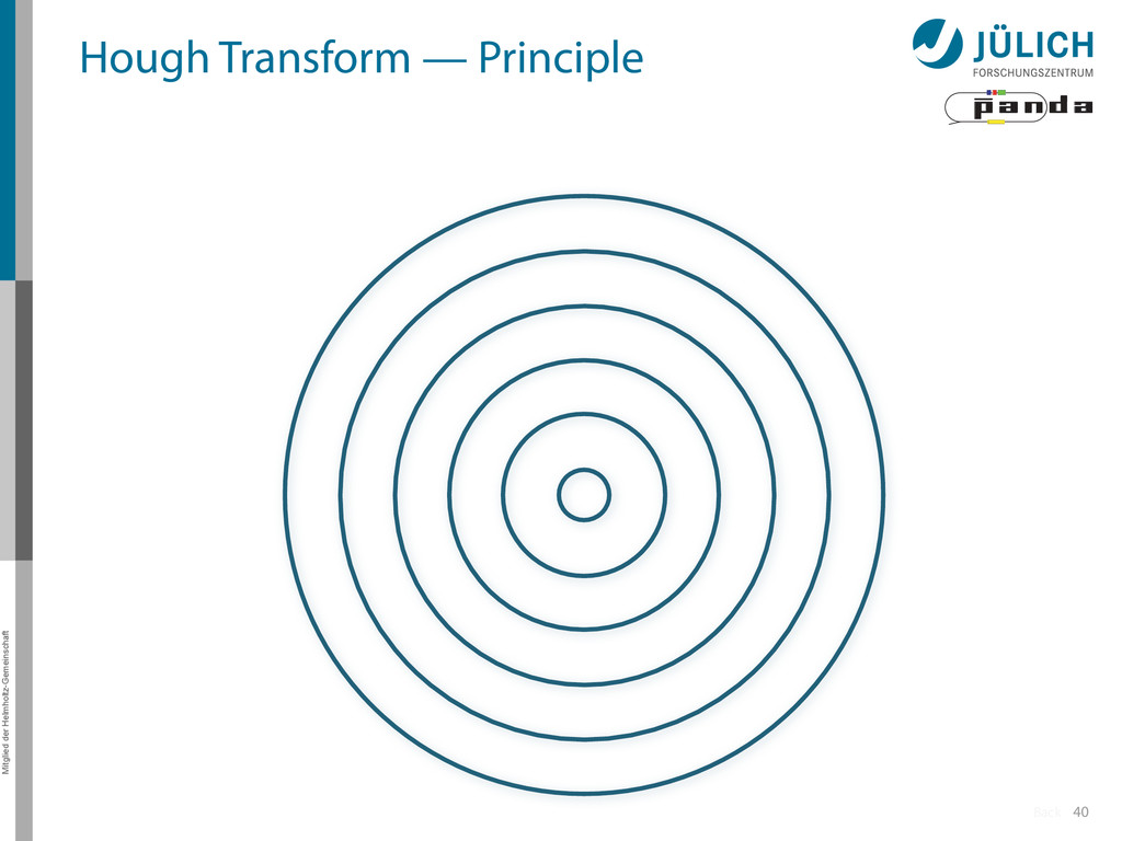
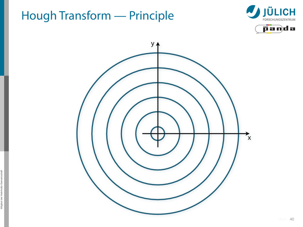
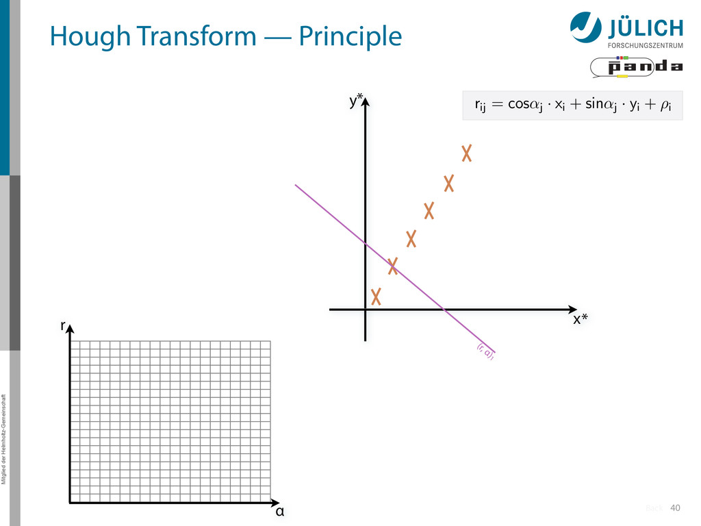
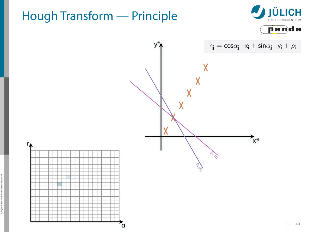
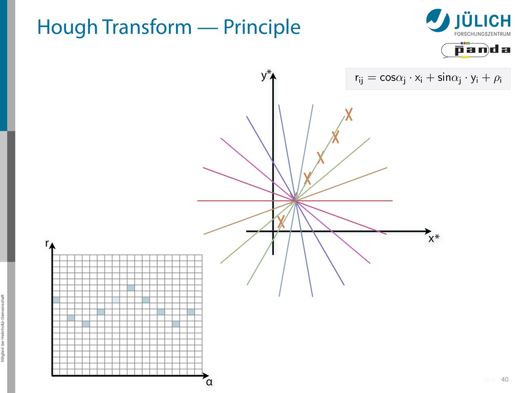
Create lines going through hit point (x,y)i – Line parameterized by rij = cos(αj ) ⋅ xi + sin(αj ) ⋅ yi • Fill line parameters (α,r)ij into histogram – Rasterize for many αj ∈ [0°,180°) α = 0°, 10°, 20°, …
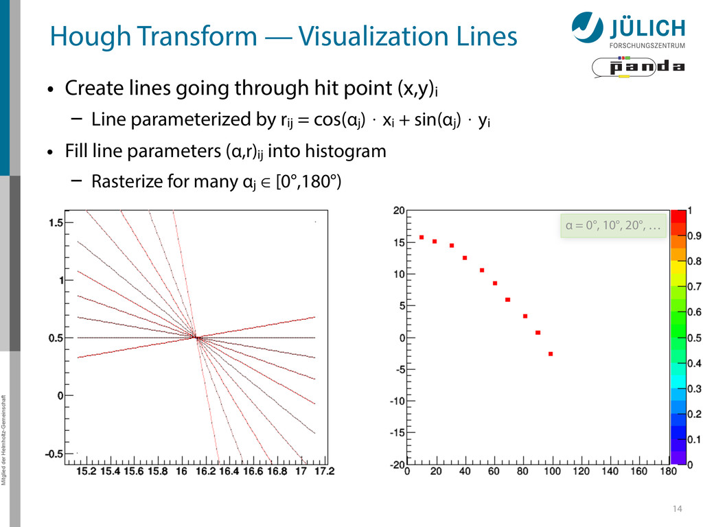
Create lines going through hit point (x,y)i – Line parameterized by rij = cos(αj ) ⋅ xi + sin(αj ) ⋅ yi • Fill line parameters (α,r)ij into histogram – Rasterize for many αj ∈ [0°,180°) α = 0°, 10°, 20°, …
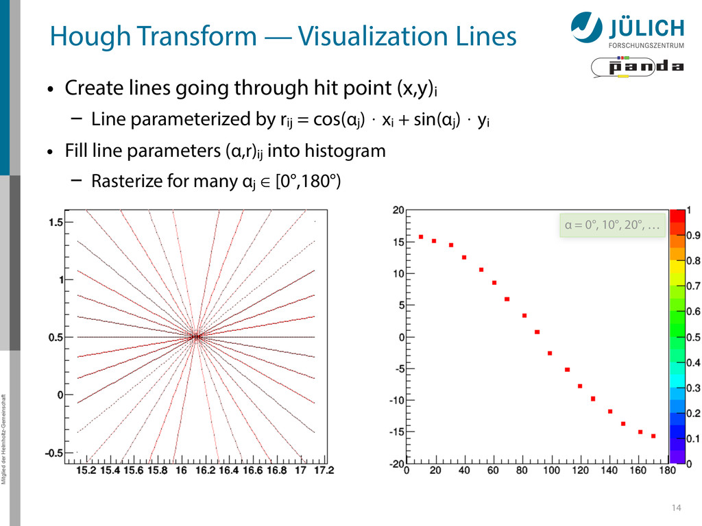
Create lines going through hit point (x,y)i – Line parameterized by rij = cos(αj ) ⋅ xi + sin(αj ) ⋅ yi • Fill line parameters (α,r)ij into histogram – Rasterize for many αj ∈ [0°,180°) α = 0°, 10°, 20°, …
Create lines going through hit point (x,y)i – Line parameterized by rij = cos(αj ) ⋅ xi + sin(αj ) ⋅ yi • Fill line parameters (α,r)ij into histogram – Rasterize for many αj ∈ [0°,180°) α = 0°, 10°, 20°, …
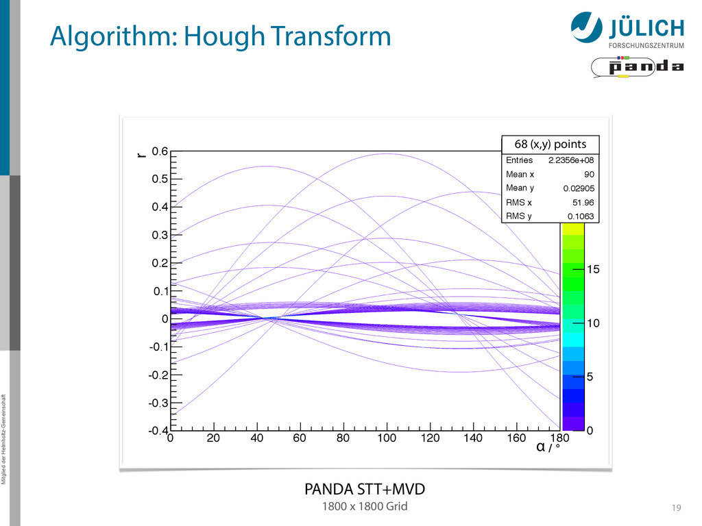
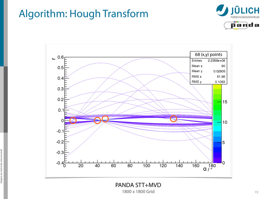
140 160 180 Hough transformed -0.4 -0.3 -0.2 -0.1 0 0.1 0.2 0.3 0.4 0.5 0.6 0 Entries 2.2356e+08 Mean x 90 Mean y 0.02905 RMS x 51.96 RMS y 0.1063 0 5 10 15 20 25 0 Entries 2.2356e+08 Mean x 90 Mean y 0.02905 RMS x 51.96 RMS y 0.1063 1800 x 1800 Grid PANDA STT+MVD Mitglied der Helmholtz-Gemeinschaft 19 68 (x,y) points r α Algorithm: Hough Transform
140 160 180 Hough transformed -0.4 -0.3 -0.2 -0.1 0 0.1 0.2 0.3 0.4 0.5 0.6 0 Entries 2.2356e+08 Mean x 90 Mean y 0.02905 RMS x 51.96 RMS y 0.1063 0 5 10 15 20 25 0 Entries 2.2356e+08 Mean x 90 Mean y 0.02905 RMS x 51.96 RMS y 0.1063 1800 x 1800 Grid PANDA STT+MVD Mitglied der Helmholtz-Gemeinschaft 19 68 (x,y) points r α Algorithm: Hough Transform
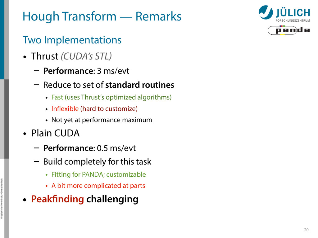
Thrust (CUDA‘s STL) – Performance: 3 ms/evt – Reduce to set of standard routines • Fast (uses Thrust‘s optimized algorithms) • Inflexible (hard to customize) • Not yet at performance maximum • Plain CUDA – Performance: 0.5 ms/evt – Build completely for this task • Fitting for PANDA; customizable • A bit more complicated at parts • 20 Peakfinding challenging
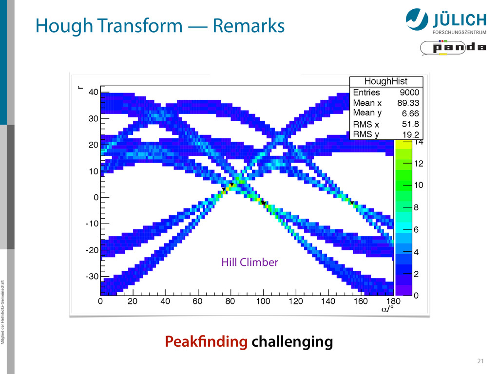
α 0 20 40 60 80 100 120 140 160 180 r -30 -20 -10 0 10 20 30 40 HoughHist Entries 9000 Mean x 89.33 Mean y 6.66 RMS x 51.8 RMS y 19.2 0 2 4 6 8 10 12 14 16 18 HoughHist Entries 9000 Mean x 89.33 Mean y 6.66 RMS x 51.8 RMS y 19.2 HT histogram Hill Climber Peakfinding challenging
α 0 20 40 60 80 100 120 140 160 180 r -30 -20 -10 0 10 20 30 40 houghIt0 Entries 9000 Mean x 89.33 Mean y 6.66 RMS x 51.8 RMS y 19.2 0 2 4 6 8 10 12 14 16 18 houghIt0 Entries 9000 Mean x 89.33 Mean y 6.66 RMS x 51.8 RMS y 19.2 HT histogram ° / α 0 20 40 60 80 100 120 140 160 180 r -30 -20 -10 0 10 20 30 40 houghIt1 Entries 5580 Mean x 89.6 Mean y 9.719 RMS x 51.78 RMS y 18.09 0 2 4 6 8 10 12 14 16 houghIt1 Entries 5580 Mean x 89.6 Mean y 9.719 RMS x 51.78 RMS y 18.09 HT histogram ° / α 0 20 40 60 80 100 120 140 160 180 r -30 -20 -10 0 10 20 30 houghIt2 Entries 2700 Mean x 89.13 Mean y 13.79 RMS x 51.77 RMS y 14.04 0 2 4 6 8 10 12 houghIt2 Entries 2700 Mean x 89.13 Mean y 13.79 RMS x 51.77 RMS y 14.04 HT histogram -40 -30 -20 -10 0 10 20 30 40 0 5 10 15 20 25 30 Iterative Maximum Deleter Peakfinding challenging current research
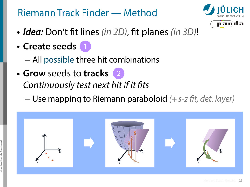
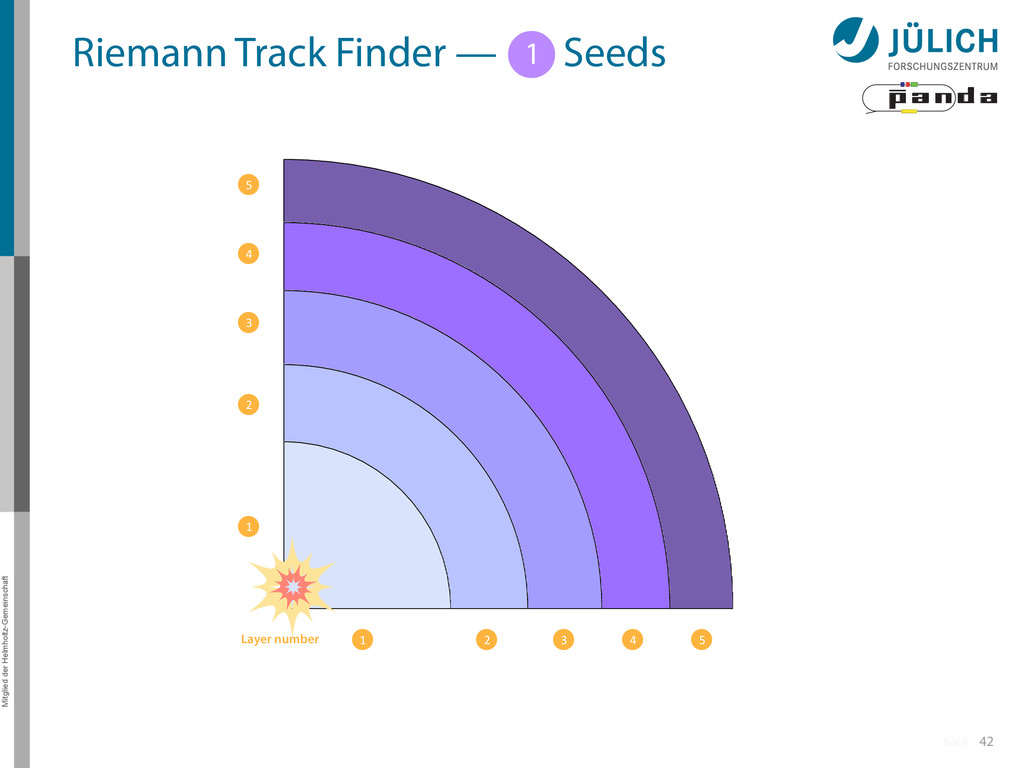
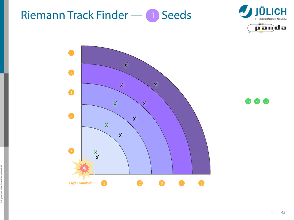
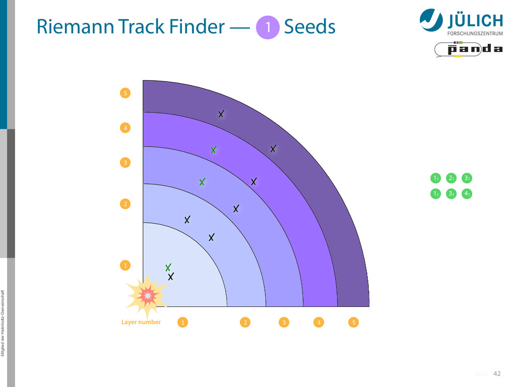
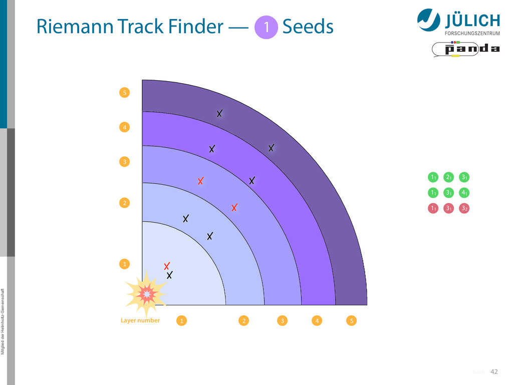
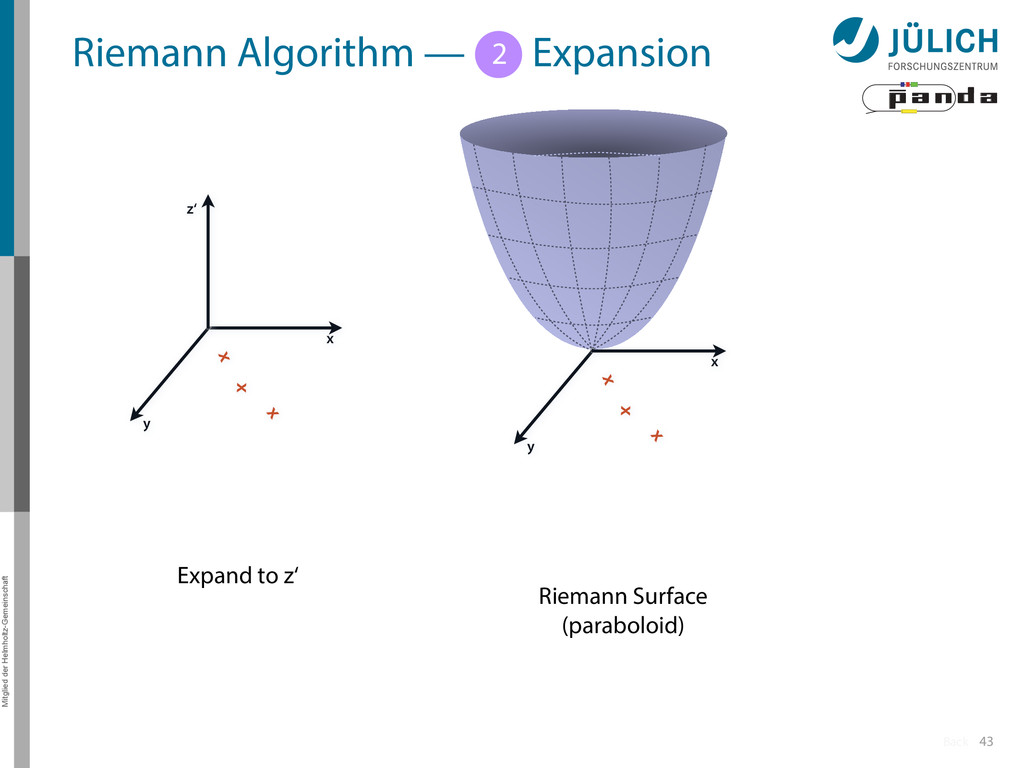
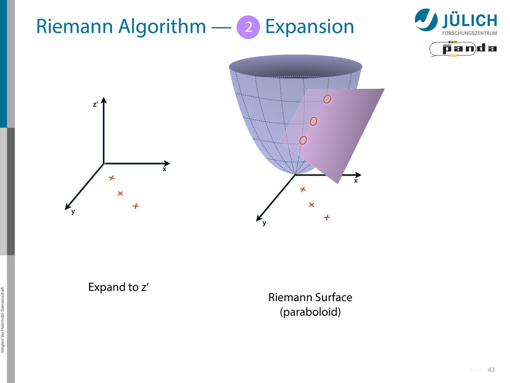
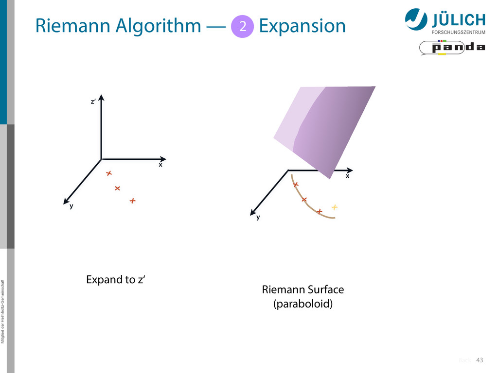
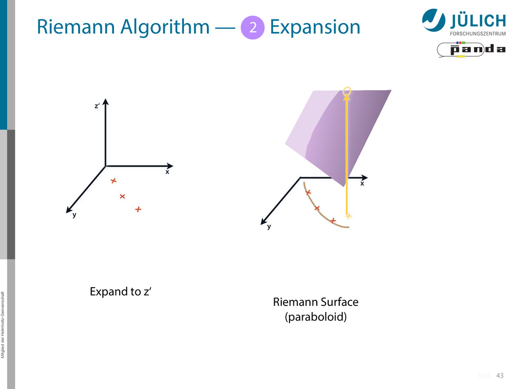
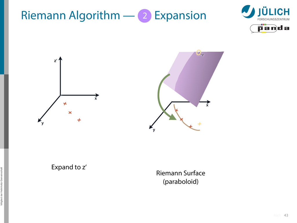
Idea: Don‘t fit lines (in 2D), fit planes (in 3D)! • Create seeds – All possible three hit combinations • Grow seeds to tracks Continuously test next hit if it fits – Use mapping to Riemann paraboloid (+ s-z fit, det. layer) x x x x y z‘ x x x y x x x x y x More on: Seeds; Growing 1 2
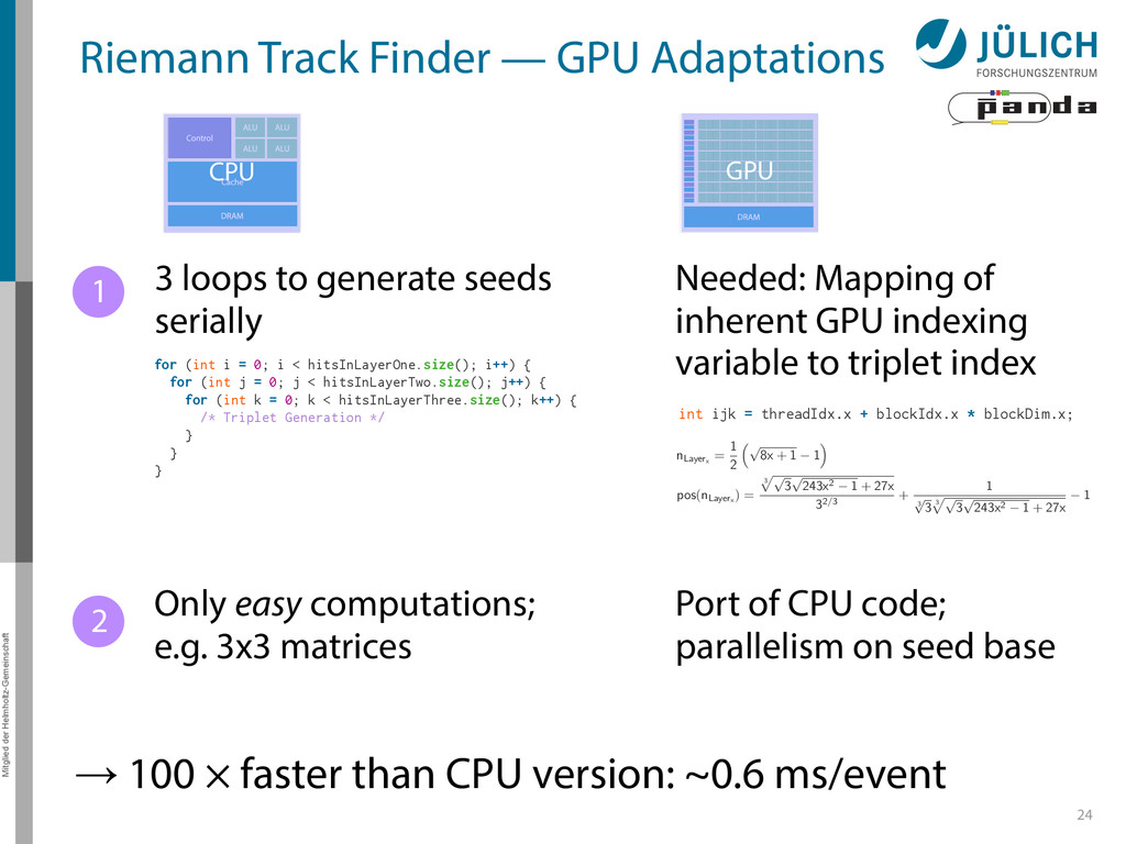
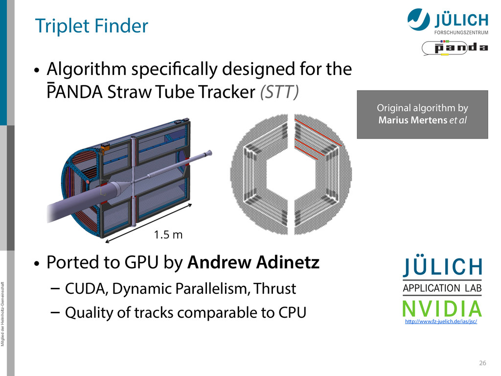
for the PANDA Straw Tube Tracker (STT) • Ported to GPU by Andrew Adinetz – CUDA, Dynamic Parallelism, Thrust – Quality of tracks comparable to CPU http://www.fz-juelich.de/ias/jsc/ Original algorithm by Marius Mertens et al 1.5 m
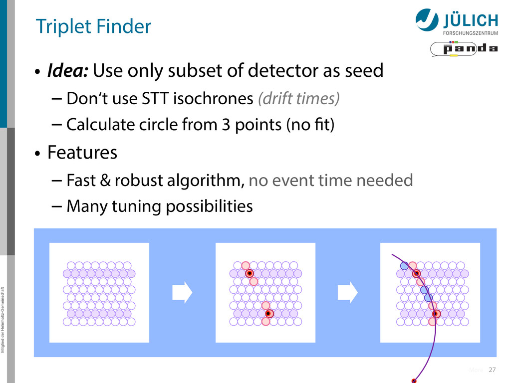
subset of detector as seed – Don‘t use STT isochrones (drift times) – Calculate circle from 3 points (no fit) • Features – Fast & robust algorithm, no event time needed – Many tuning possibilities More
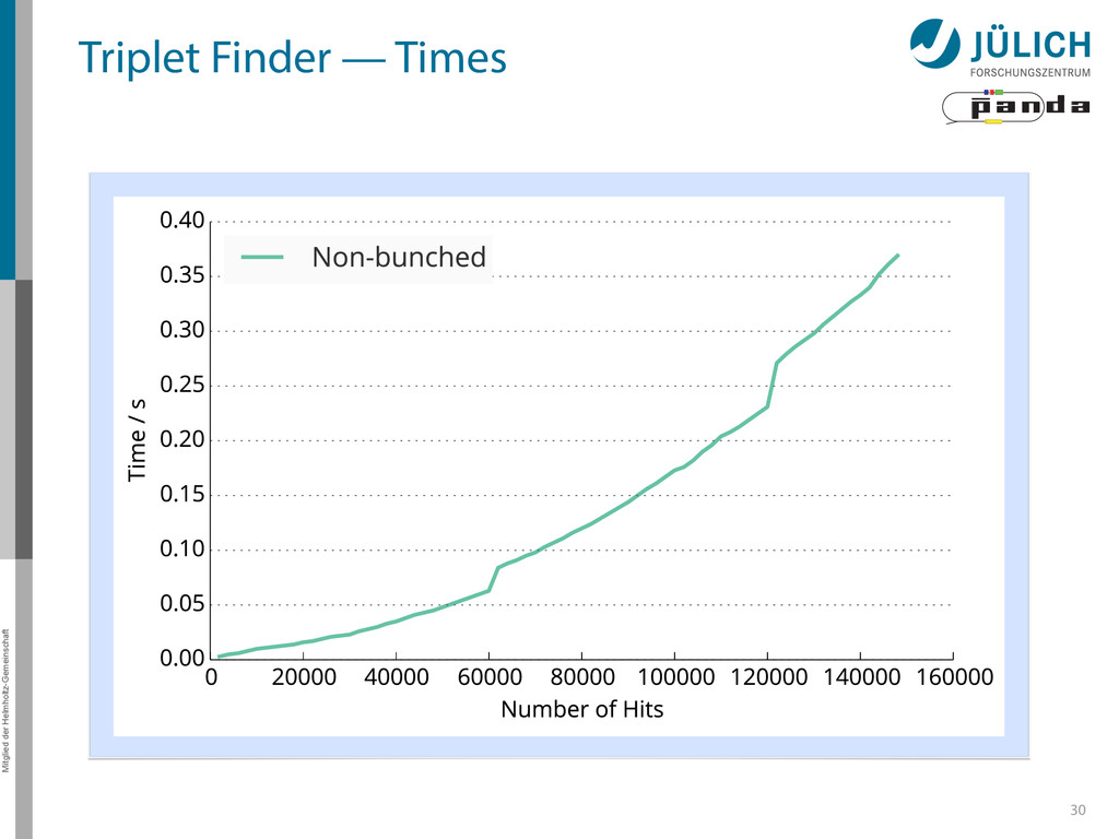
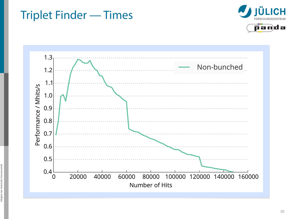
20 µs/event – 20⋅10-6 s/event * 2⋅107 event/s 㱺 400 GPUs2014 – PANDA2019: Multi GPU system – !(100) GPUs • Optimizations possible & needed – ε needs to be improved – Speed, €: • More float less double-cards a la K10 • Consumer-grade cards a la GTX 36
as part of online event reconstruction scheme • Algorithms in active evaluation and optimization – Triplet Finder performance-optimized • Data transfer to GPU in research: FairMQ → Poster by Ludovico Bianchi 37
PANDA researches in using GPUs as part of online event reconstruction scheme • Algorithms in active evaluation and optimization – Triplet Finder performance-optimized • Data transfer to GPU in research: FairMQ → Poster by Ludovico Bianchi 37
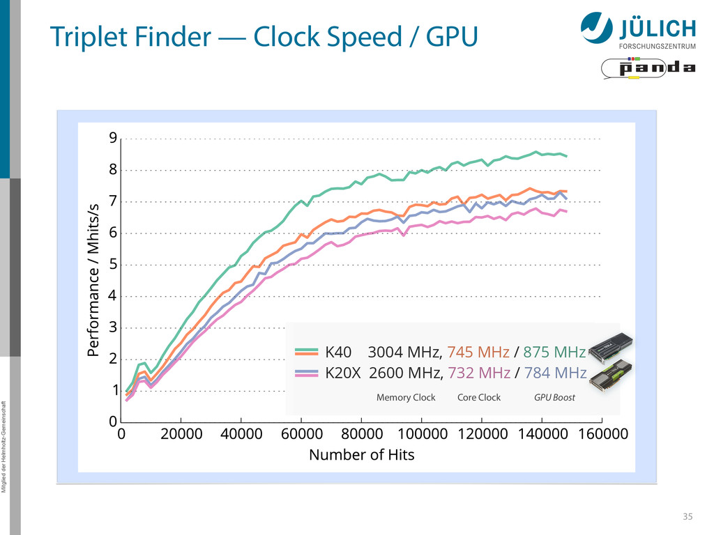
icon by Francesco Paleari from The Noun Project • #4: Einstein icon by Roman Rusinov from The Noun Project • #6: FAIR vector logo from official FAIR website • #6: FAIR rendering from official website • #11: Flare Gun icon by Jop van der Kroef from The Noun Project • #27: STT event animation by Marius C. Mertens • #35: Graphics cards images by NVIDIA promotion • #35: GPU Specifications – Tesla K20X Specifications: http://www.nvidia.com/content/PDF/kepler/Tesla- K20X-BD-06397-001-v07.pdf – Tesla K40 Specifications: http://www.nvidia.com/content/PDF/kepler/Tesla-K40- Active-Board-Spec-BD-06949-001_v03.pdf – Tesla Familiy Overview: http://www.nvidia.com/content/tesla/pdf/NVIDIA-Tesla- Kepler-Family-Datasheet.pdf 38
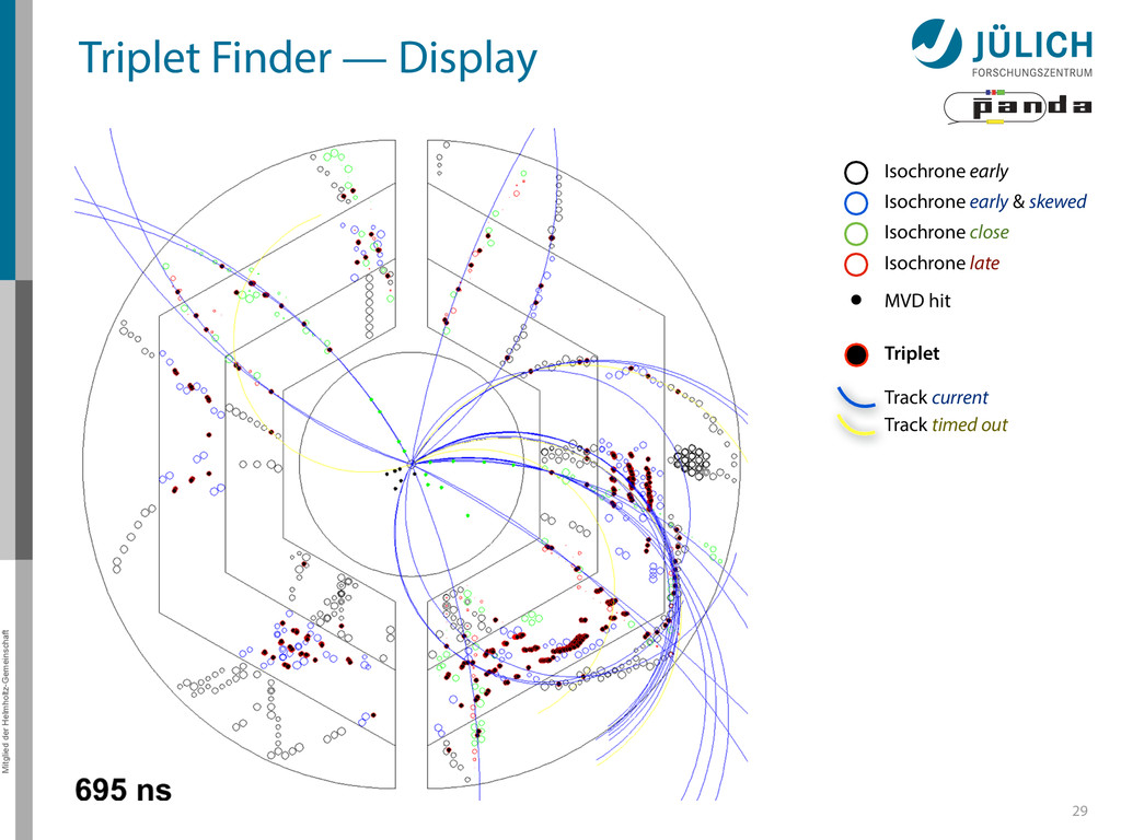
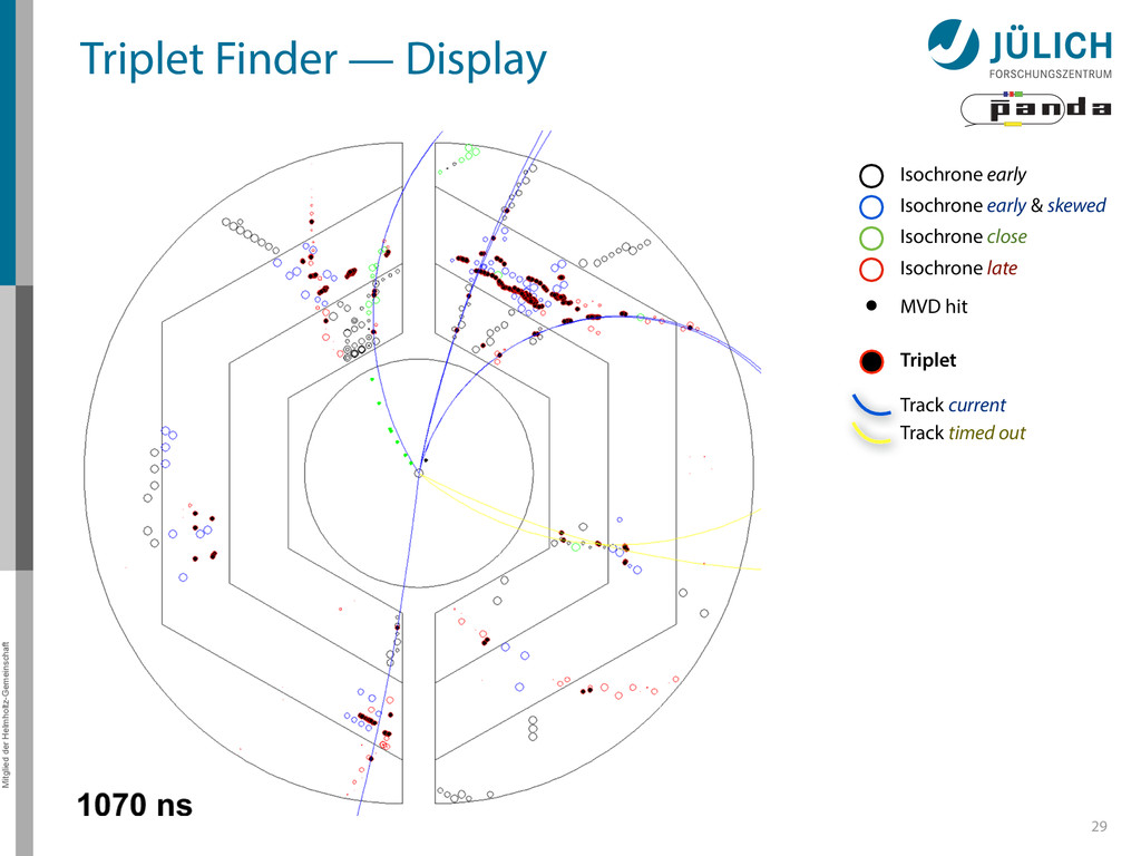
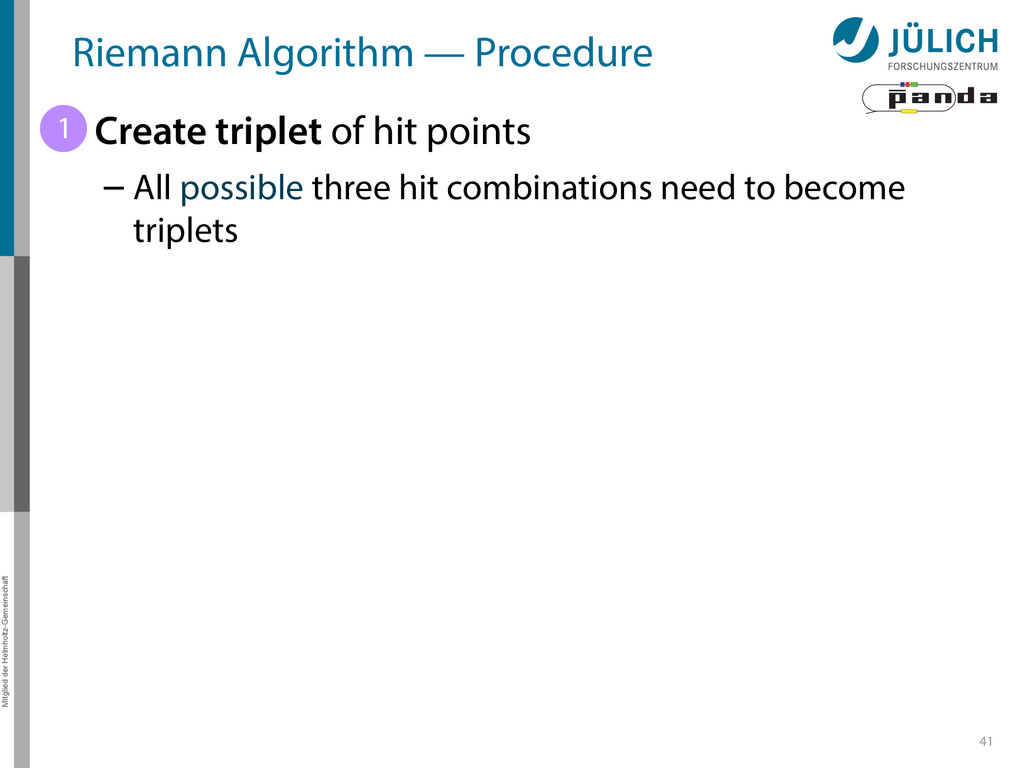
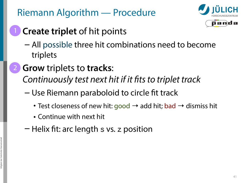
triplet of hit points – All possible three hit combinations need to become triplets • Grow triplets to tracks: Continuously test next hit if it fits to triplet track – Use Riemann paraboloid to circle fit track • Test closeness of new hit: good → add hit; bad → dismiss hit • Continue with next hit – Helix fit: arc length s vs. z position 1 2
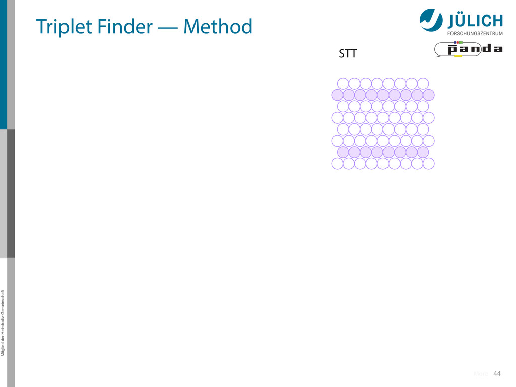
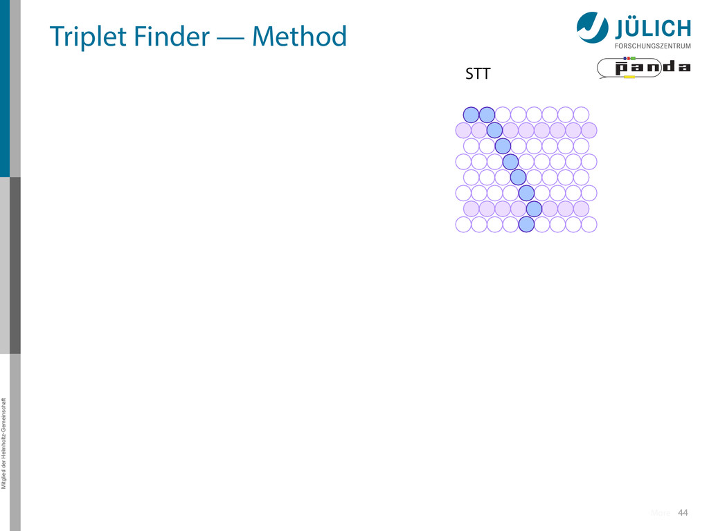
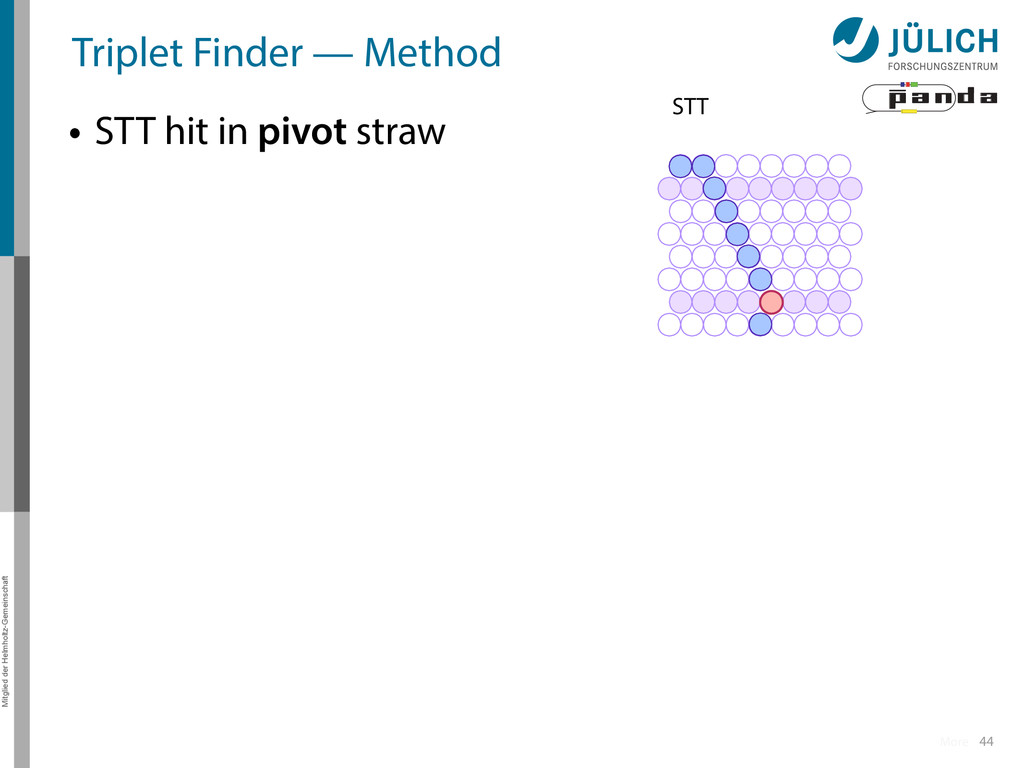
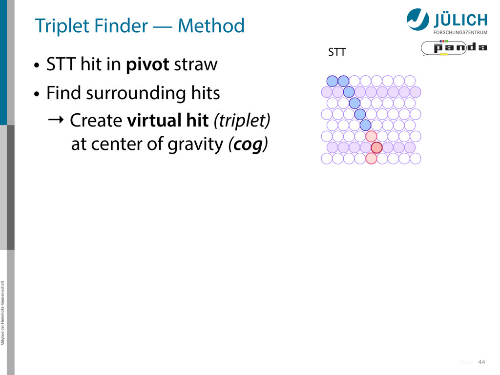
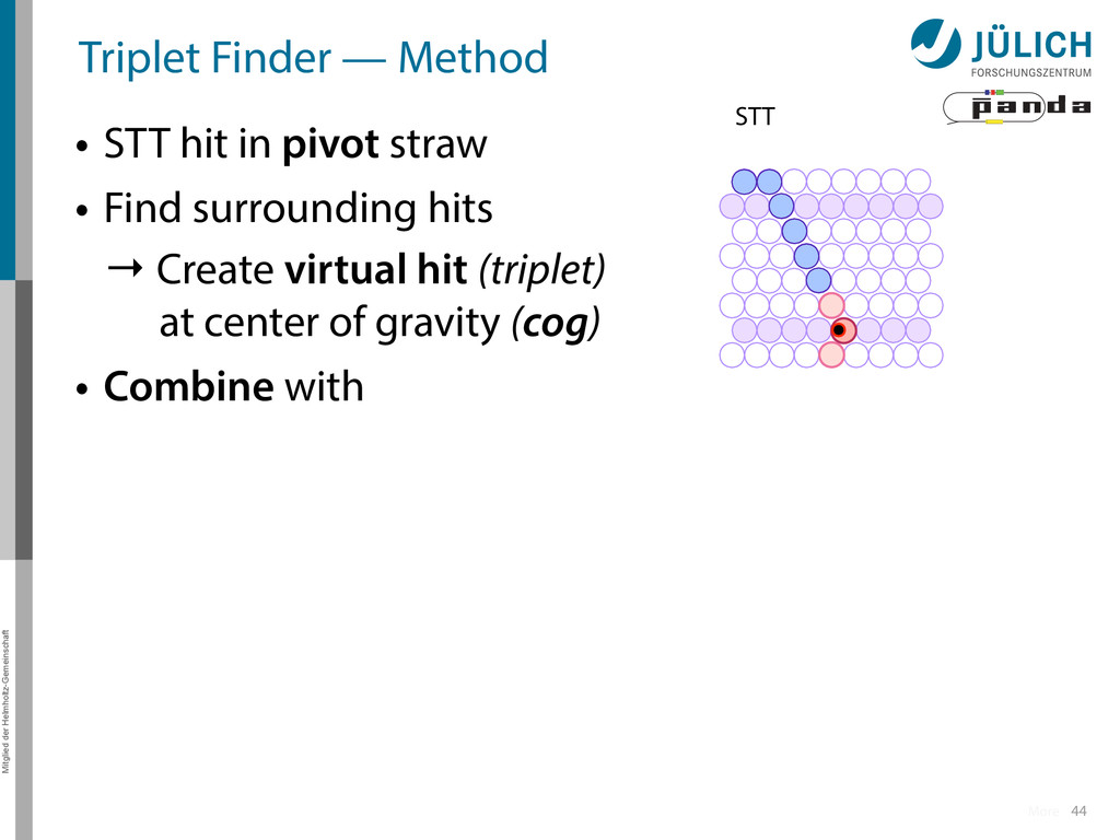
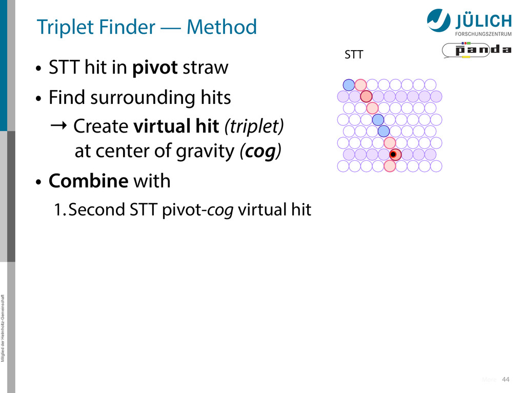
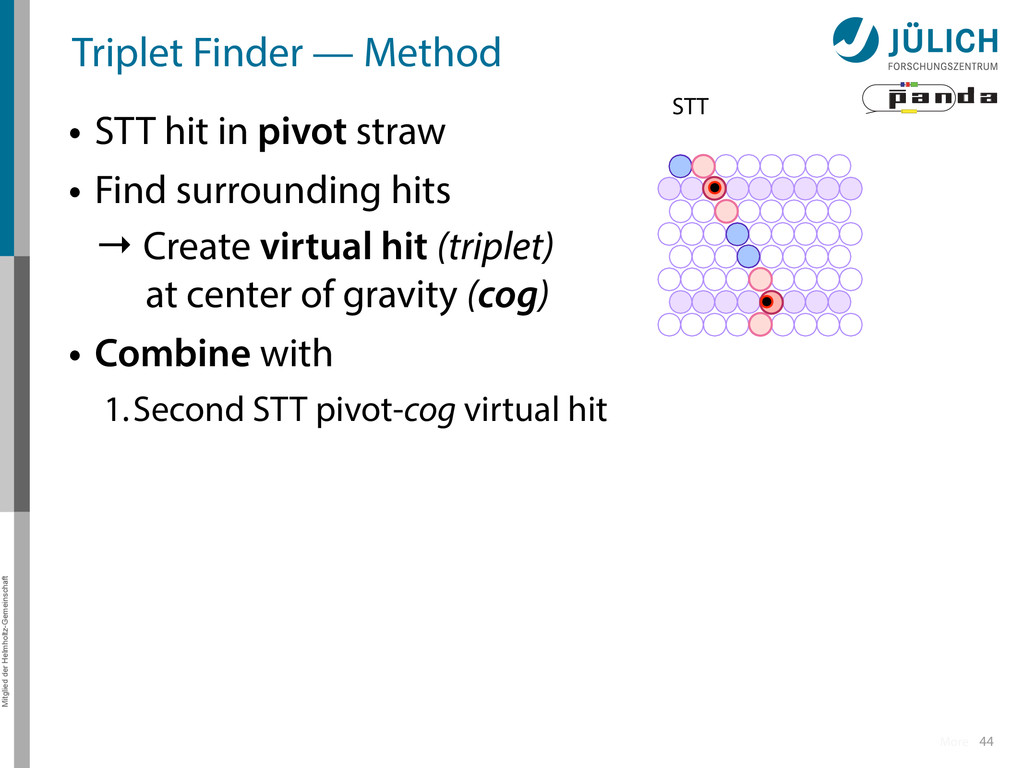
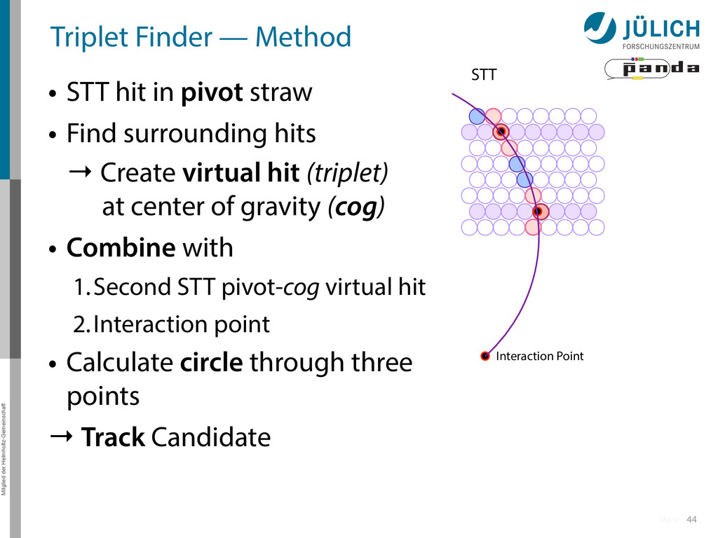
in pivot straw • Find surrounding hits → Create virtual hit (triplet) at center of gravity (cog) • Combine with 1.Second STT pivot-cog virtual hit 44 STT More
in pivot straw • Find surrounding hits → Create virtual hit (triplet) at center of gravity (cog) • Combine with 1.Second STT pivot-cog virtual hit 44 STT More
in pivot straw • Find surrounding hits → Create virtual hit (triplet) at center of gravity (cog) • Combine with 1.Second STT pivot-cog virtual hit 44 STT More
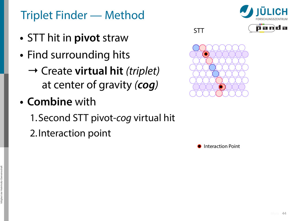
in pivot straw • Find surrounding hits → Create virtual hit (triplet) at center of gravity (cog) • Combine with 1.Second STT pivot-cog virtual hit 2.Interaction point 44 Interaction Point STT More
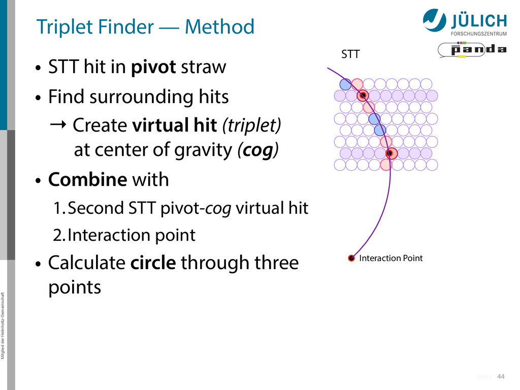
in pivot straw • Find surrounding hits → Create virtual hit (triplet) at center of gravity (cog) • Combine with 1.Second STT pivot-cog virtual hit 2.Interaction point • Calculate circle through three points 44 Interaction Point STT More
in pivot straw • Find surrounding hits → Create virtual hit (triplet) at center of gravity (cog) • Combine with 1.Second STT pivot-cog virtual hit 2.Interaction point • Calculate circle through three points → Track Candidate 44 Interaction Point STT More
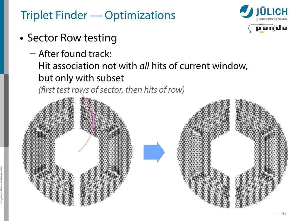
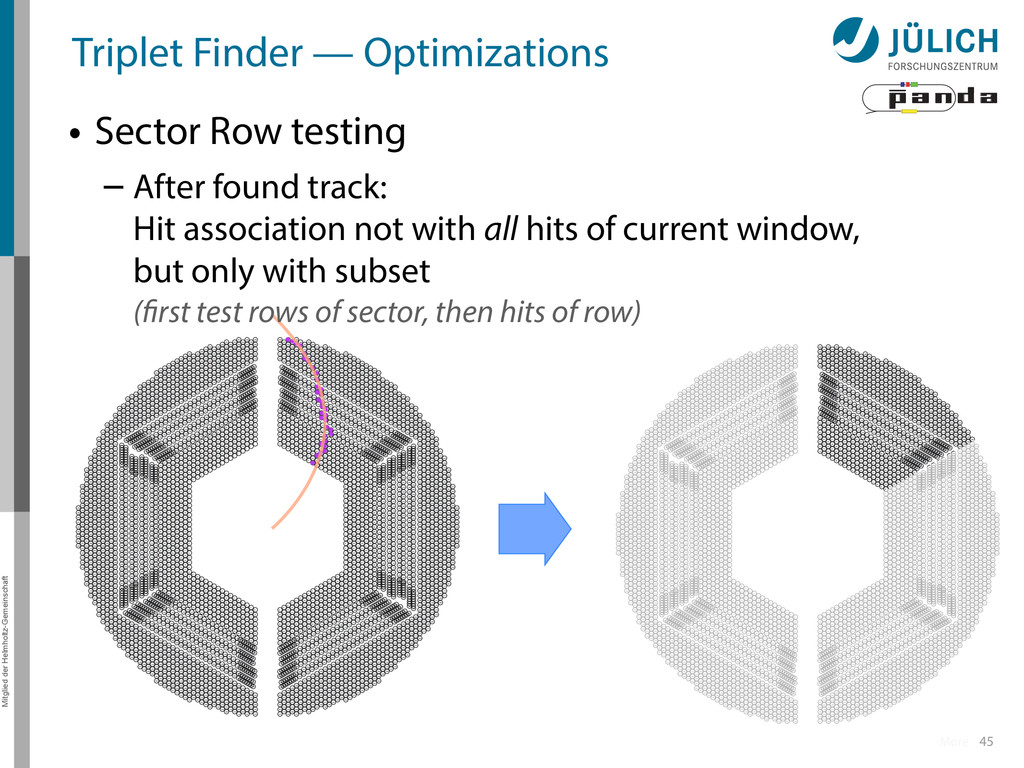
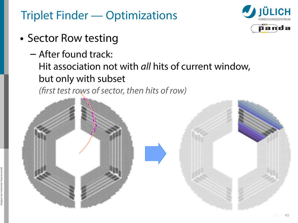
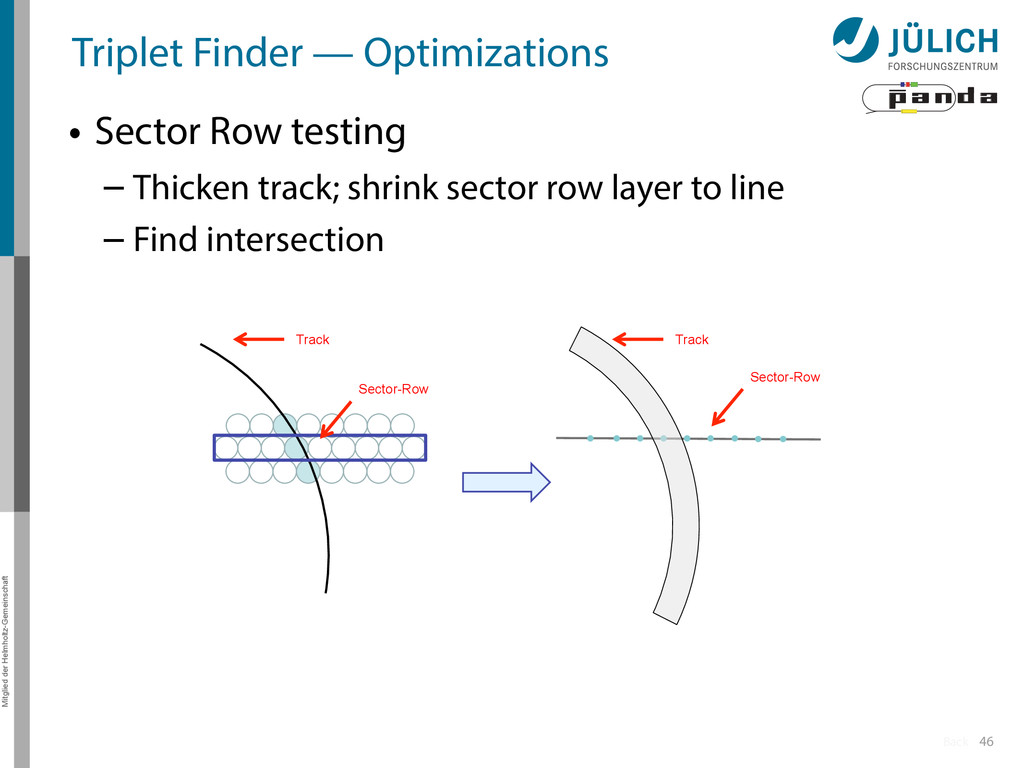
Row testing – After found track: Hit association not with all hits of current window, but only with subset (first test rows of sector, then hits of row) More
Row testing – After found track: Hit association not with all hits of current window, but only with subset (first test rows of sector, then hits of row) More
Row testing – After found track: Hit association not with all hits of current window, but only with subset (first test rows of sector, then hits of row) More
Row testing – After found track: Hit association not with all hits of current window, but only with subset (first test rows of sector, then hits of row) More
Row testing – After found track: Hit association not with all hits of current window, but only with subset (first test rows of sector, then hits of row) More
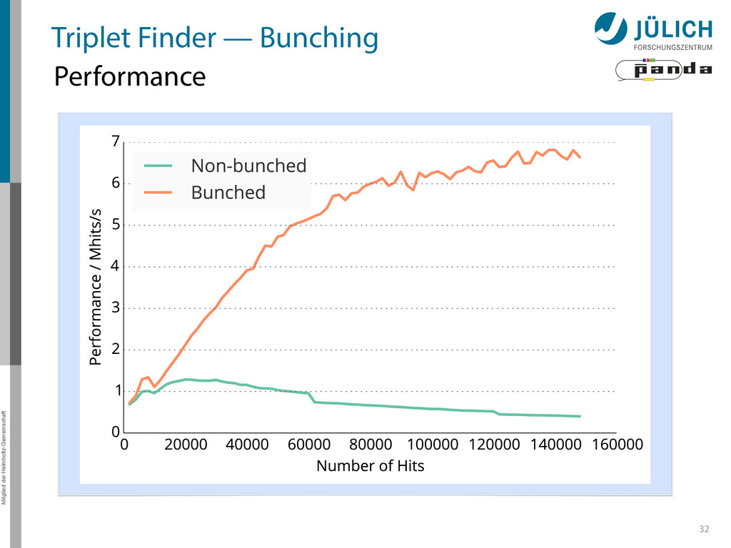
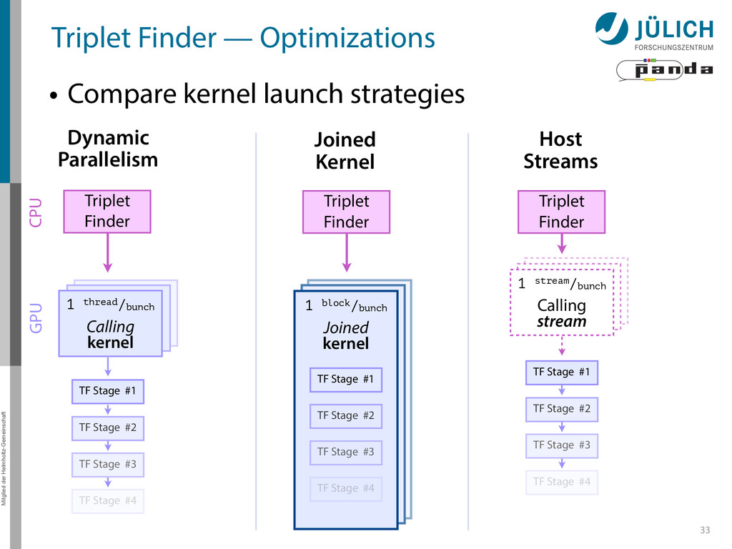
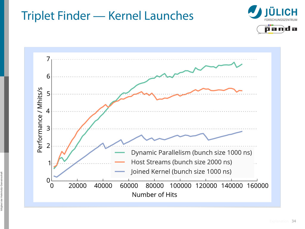
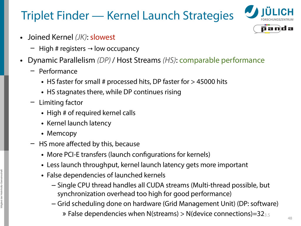
Joined Kernel (JK): slowest – High # registers → low occupancy • Dynamic Parallelism (DP) / Host Streams (HS): comparable performance – Performance • HS faster for small # processed hits, DP faster for > 45000 hits • HS stagnates there, while DP continues rising – Limiting factor • High # of required kernel calls • Kernel launch latency • Memcopy – HS more affected by this, because • More PCI-E transfers (launch configurations for kernels) • Less launch throughput, kernel launch latency gets more important • False dependencies of launched kernels – Single CPU thread handles all CUDA streams (Multi-thread possible, but synchronization overhead too high for good performance) – Grid scheduling done on hardware (Grid Management Unit) (DP: software) » False dependencies when N(streams) > N(device connections)=323.5 48 Back
![Thank you! Andreas Herten [email protected] Mitglied der Helmholtz-Gemeinschaft Summary •](https://files.speakerdeck.com/presentations/ac131340382101323fa21a5a9fa5ab8d/slide_69.jpg)