Error and Attack Tolerance in Public Transport Networks: A Temporal Networks Approach

Measuring reachability of a public transportation network modelled as a temporal network and performing targeted and random attacks to understand its structure.

Transcript

1. Error and Attack Tolerance in Public Transport Networks: A Temporal Networks Approach Arash Badie Modiri Supervisor + Advisor: Mikko Kivelä The tramway carriage to Munkkiniemi — 1952. Helsinki City Museum
2. Networks as models A network is a set of nodes V and a set of links E where each member of E is an unordered pair of node indicating that they are connected. We can always add more details back in, but the challenge is to find the most simple, most universal model that gives the most accurate predictions of properties of the real-world phenomena.
3. Robustness of networks Removing parts of the network one by one and observing evolution of properties of the network: e.g. diameter or size of largest component. • Understanding and comparing vulnerability of different systems • Understanding role of structures and inhomogeneities in connectivity of the network.
4. Robustness of networks Removing parts of the network one by one and observing evolution of properties of the network: e.g. diameter or size of largest component. • Understanding and comparing vulnerability of different systems • Understanding role of structures and inhomogeneities in connectivity of the network.
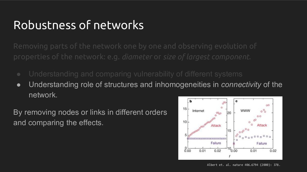
5. Robustness of networks Removing parts of the network one by one and observing evolution of properties of the network: e.g. diameter or size of largest component. • Understanding and comparing vulnerability of different systems • Understanding role of structures and inhomogeneities in connectivity of the network. By removing nodes or links in different orders and comparing the effects. Albert et. al. nature 406.6794 (2000): 378.
6. Temporal Networks Same definition as “static” networks, except now each link comes with a set of timestamps that determine when it is active. • Static network is the simpler model • Difference in observable implications?
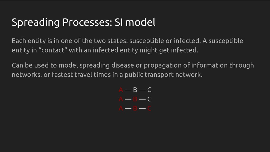
7. Spreading Processes: SI model Each entity is in one of the two states: susceptible or infected. A susceptible entity in “contact” with an infected entity might get infected. Can be used to model spreading disease or propagation of information through networks, or fastest travel times in a public transport network. A — B — C A — B — C A — B — C
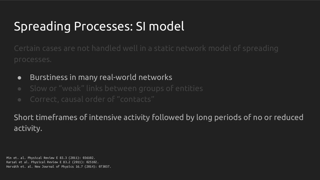
8. Spreading Processes: SI model Certain cases are not handled well in a static network model of spreading processes. • Burstiness in many real-world networks • Slow or “weak” links between groups of entities • Correct, causal order of “contacts”
9. Spreading Processes: SI model Certain cases are not handled well in a static network model of spreading processes. • Burstiness in many real-world networks • Slow or “weak” links between groups of entities • Correct, causal order of “contacts” Short timeframes of intensive activity followed by long periods of no or reduced activity. Min et. al. Physical Review E 83.3 (2011): 036102. Karsai et al. Physical Review E 83.2 (2011): 025102. Horváth et. al. New Journal of Physics 16.7 (2014): 073037.
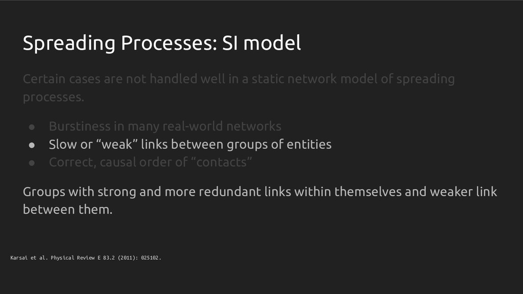
10. Spreading Processes: SI model Certain cases are not handled well in a static network model of spreading processes. • Burstiness in many real-world networks • Slow or “weak” links between groups of entities • Correct, causal order of “contacts” Groups with strong and more redundant links within themselves and weaker link between them. Karsai et al. Physical Review E 83.2 (2011): 025102.
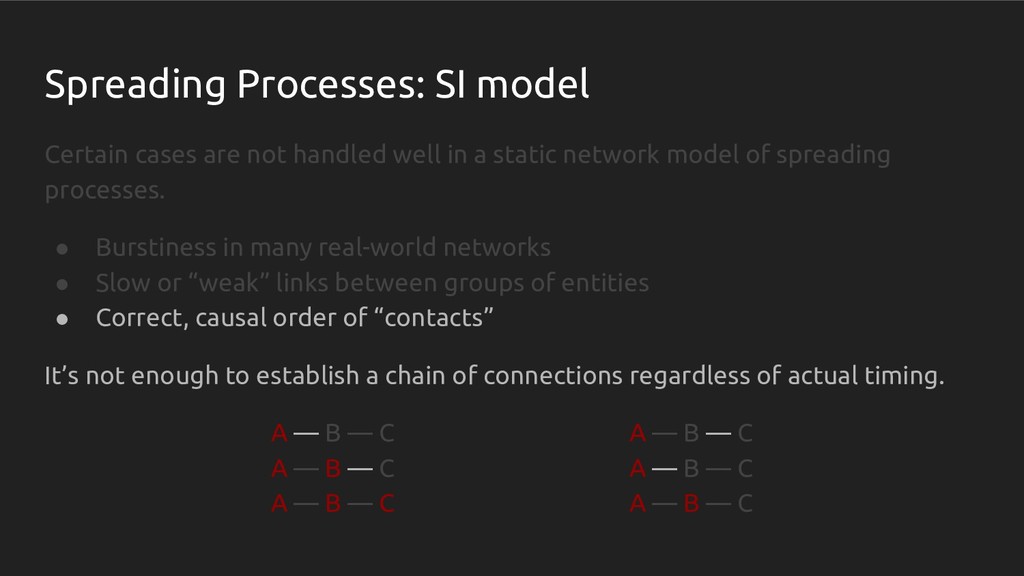
11. Spreading Processes: SI model Certain cases are not handled well in a static network model of spreading processes. • Burstiness in many real-world networks • Slow or “weak” links between groups of entities • Correct, causal order of “contacts” It’s not enough to establish a chain of connections regardless of actual timing. A — B — C A — B — C A — B — C A — B — C A — B — C A — B — C
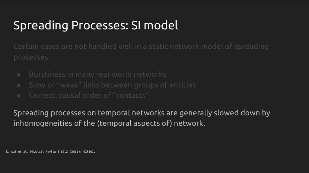
12. Spreading Processes: SI model Certain cases are not handled well in a static network model of spreading processes. • Burstiness in many real-world networks • Slow or “weak” links between groups of entities • Correct, causal order of “contacts” Spreading processes on temporal networks are generally slowed down by inhomogeneities of the (temporal aspects of) network. Karsai et al. Physical Review E 83.2 (2011): 025102.
13. Temporal Networks: Public Transportation Nodes: set of stops Links: connections; vehicles moving from one stop to the next SI model on temporal network model of public transportation can show how fast a passenger can travel from one stop to all other stops. We need to add one more bit of information: walking between stops.
14. Temporal Networks: Public Transportation Nodes: set of stops Links: connections; vehicles moving from one stop to the next SI model on temporal network model of public transportation can show how fast a passenger can travel from one stop to all other stops. We need to add one more bit of information: walking between stops.
15. Temporal Networks: Public Transportation Nodes: set of stops Links: connections; vehicles moving from one stop to the next SI model on temporal network model of public transportation can show how fast a passenger can travel from one stop to all other stops. We need to add one more bit of information: walking between stops.
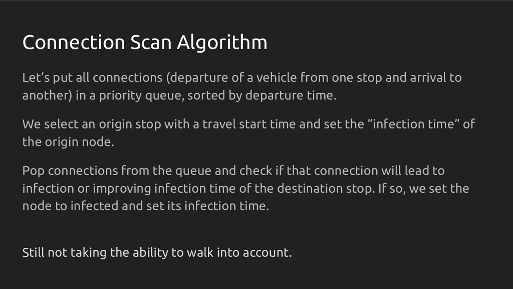
16. Connection Scan Algorithm Let’s put all connections (departure of a vehicle from one stop and arrival to another) in a priority queue, sorted by departure time. We select an origin stop with a travel start time and set the “infection time” of the origin node. Pop connections from the queue and check if that connection will lead to infection or improving infection time of the destination stop. If so, we set the node to infected and set its infection time.
17. Connection Scan Algorithm Let’s put all connections (departure of a vehicle from one stop and arrival to another) in a priority queue, sorted by departure time. We select an origin stop with a travel start time and set the “infection time” of the origin node. Pop connections from the queue and check if that connection will lead to infection or improving infection time of the destination stop. If so, we set the node to infected and set its infection time. Still not taking the ability to walk into account.
18. Connection Scan Algorithm, continued Each time we update infection time of a node, we create pseudo-connection based on walking from that node to nearby stops, departing at the new infection time and arriving after however long it takes walking the distance. We then just push them in the priority queue like any other connection.
19. Connection Scan Algorithm, continued Improvement: What if instead of recording an infection time for each node, we record an infecting connection. We can then create a chain of these connection, a shortest path, going all the way back to the origin.
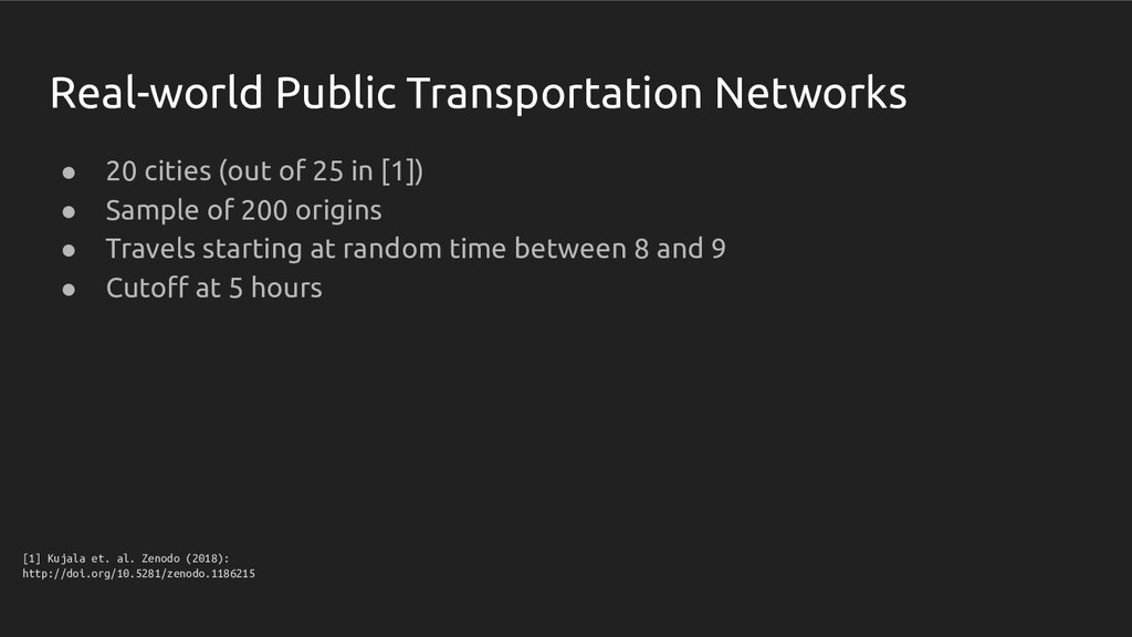
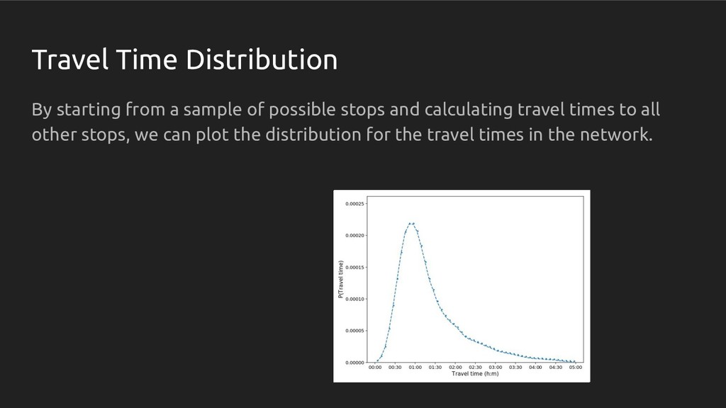
20. Real-world Public Transportation Networks • 20 cities (out of 25 in [1]) • Sample of 200 origins • Travels starting at random time between 8 and 9 • Cutoff at 5 hours [1] Kujala et. al. Zenodo (2018): http://doi.org/10.5281/zenodo.1186215
21. Travel Time Distribution By starting from a sample of possible stops and calculating travel times to all other stops, we can plot the distribution for the travel times in the network.
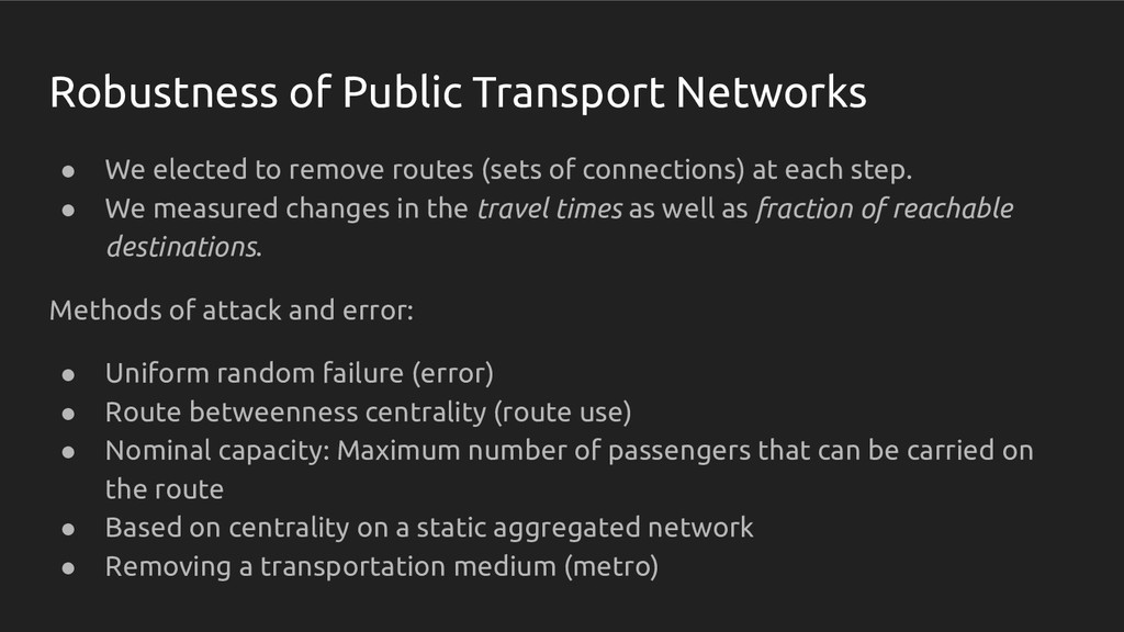
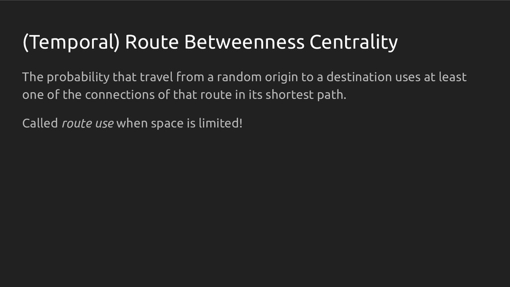
22. Robustness of Public Transport Networks • We elected to remove routes (sets of connections) at each step. • We measured changes in the travel times as well as fraction of reachable destinations. Methods of attack and error: • Uniform random failure (error) • Route betweenness centrality (route use) • Nominal capacity: Maximum number of passengers that can be carried on the route • Based on centrality on a static aggregated network • Removing a transportation medium (metro)
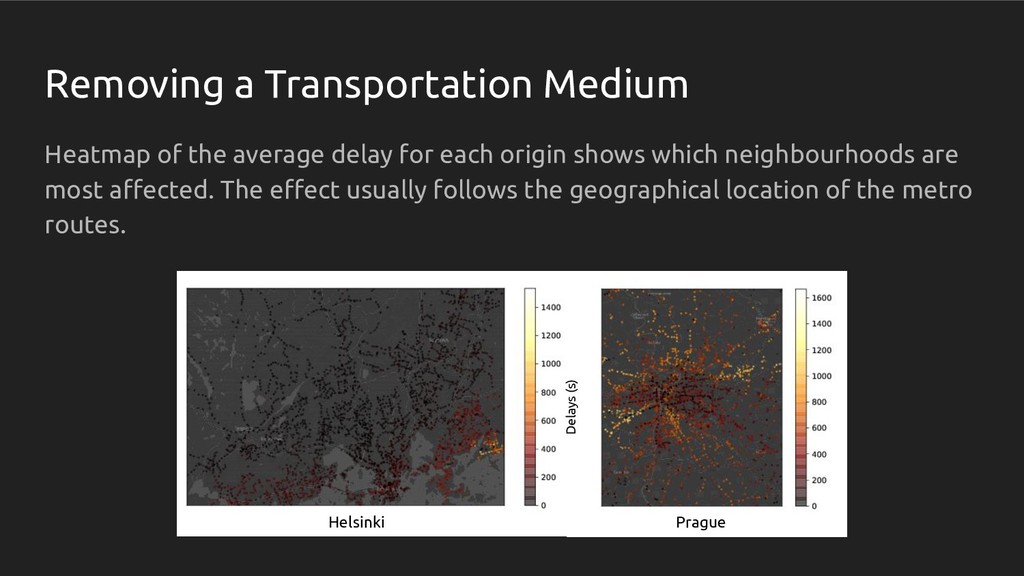
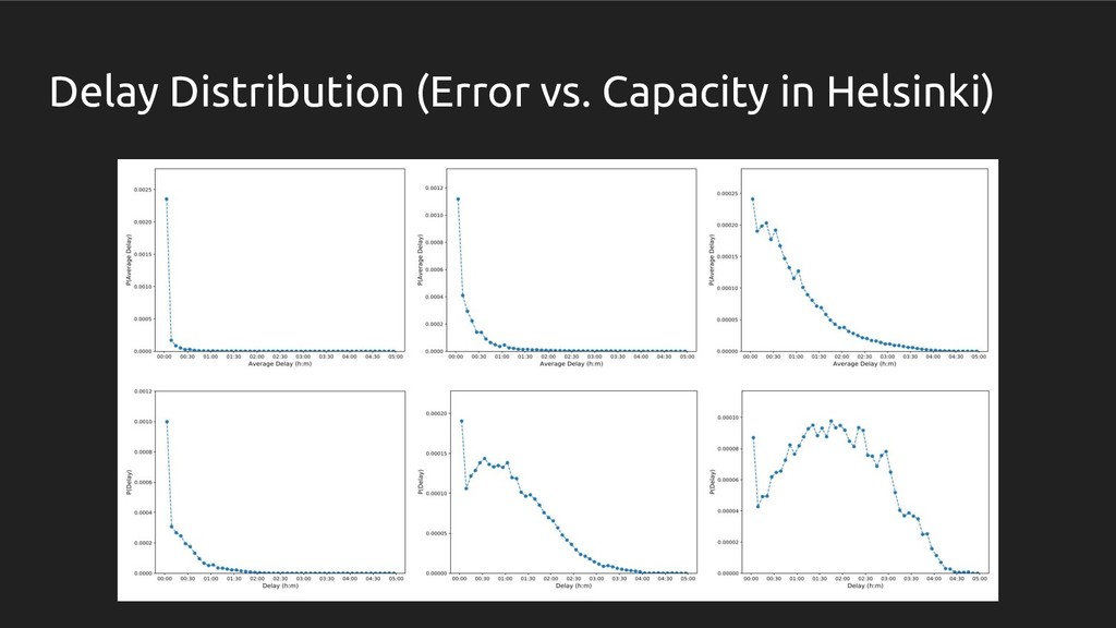
23. Removing a Transportation Medium Heatmap of the average delay for each origin shows which neighbourhoods are most affected. The effect usually follows the geographical location of the metro routes. Helsinki Prague Delays (s)
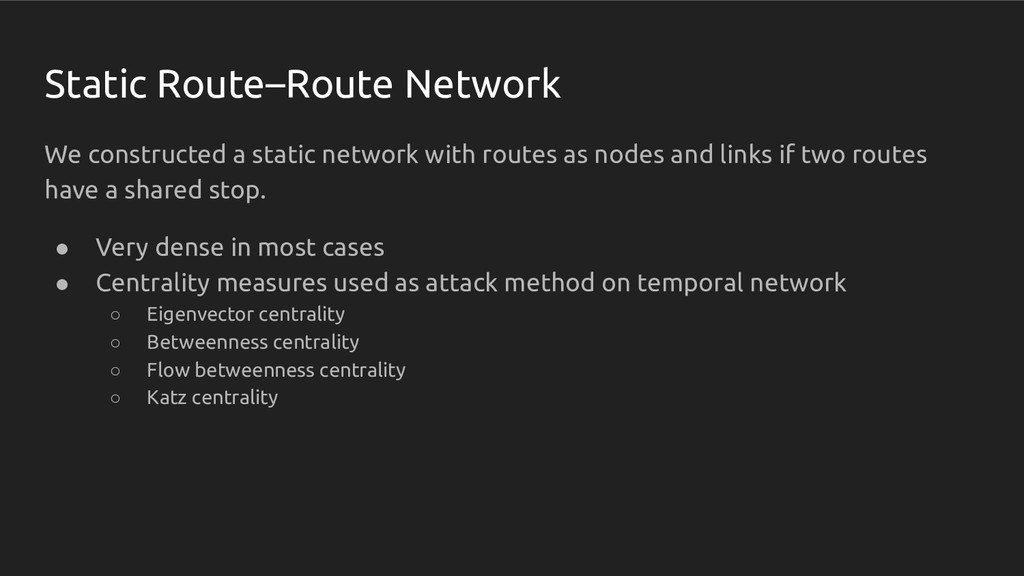
24. Static Route–Route Network We constructed a static network with routes as nodes and links if two routes have a shared stop. • Very dense in most cases • Centrality measures used as attack method on temporal network ◦ Eigenvector centrality ◦ Betweenness centrality ◦ Flow betweenness centrality ◦ Katz centrality
25. (Temporal) Route Betweenness Centrality The probability that travel from a random origin to a destination uses at least one of the connections of that route in its shortest path. Called route use when space is limited!
26. Delay Distribution (Error vs. Capacity in Helsinki)
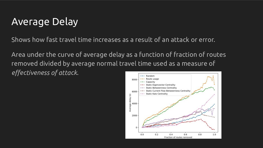
27. Average Delay Shows how fast travel time increases as a result of an attack or error. Area under the curve of average delay as a function of fraction of routes removed divided by average normal travel time used as a measure of effectiveness of attack.
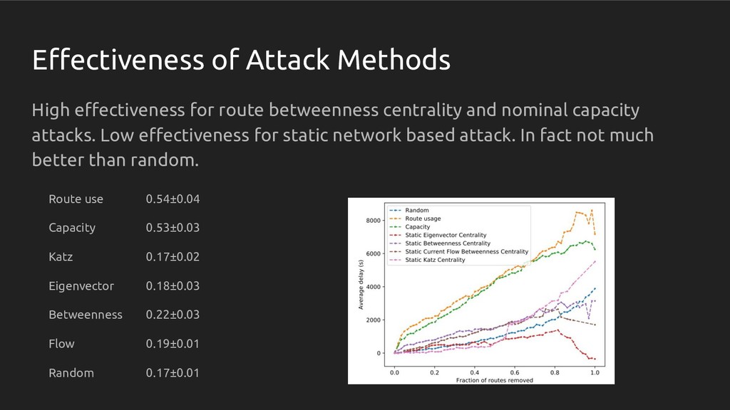
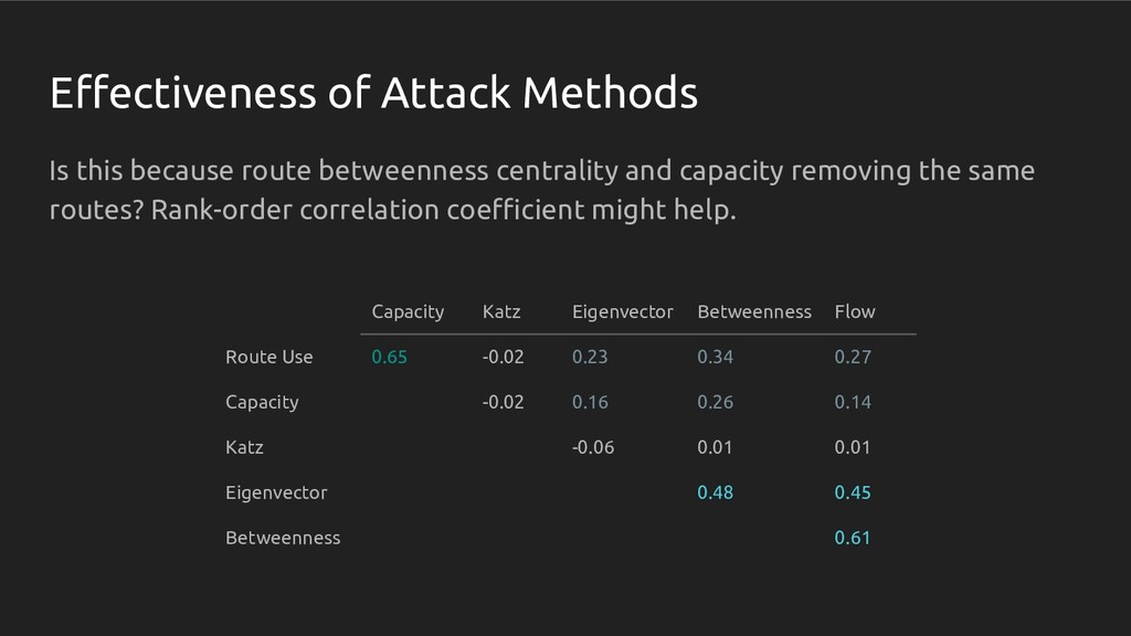
28. Effectiveness of Attack Methods High effectiveness for route betweenness centrality and nominal capacity attacks. Low effectiveness for static network based attack. In fact not much better than random. Route use 0.54±0.04 Capacity 0.53±0.03 Katz 0.17±0.02 Eigenvector 0.18±0.03 Betweenness 0.22±0.03 Flow 0.19±0.01 Random 0.17±0.01
29. Effectiveness of Attack Methods Capacity Katz Eigenvector Betweenness Flow Route Use 0.65 -0.02 0.23 0.34 0.27 Capacity -0.02 0.16 0.26 0.14 Katz -0.06 0.01 0.01 Eigenvector 0.48 0.45 Betweenness 0.61 Is this because route betweenness centrality and capacity removing the same routes? Rank-order correlation coefficient might help.
30. Effectiveness of Attack Methods Route betweenness centrality and nominal capacity are not removing the route with the same order, although this level of correlation suggests that there are many similarities. Static measures (except Katz) also had significant correlations between themselves, but using a static aggregate network like this to devise attacks simply doesn’t seem to work that well.
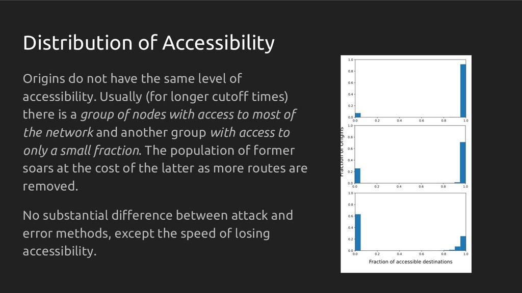
31. Accessibility A measure of “ease of access” from origins to destinations. We used the fraction of reachable destinations of an origin within a certain time limit as a measure of accessibility. Lack of accessibility is counted as a factor contributing to social exclusion.
32. Accessibility Similar to delays, accessibility is also reduced much faster with nominal capacity and route betweenness centrality attack method compared to uniform random removal.
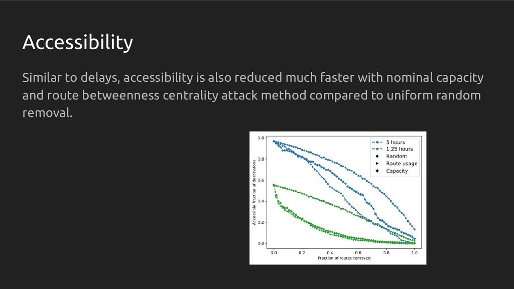
33. Distribution of Accessibility Origins do not have the same level of accessibility. Usually (for longer cutoff times) there is a group of nodes with access to most of the network and another group with access to only a small fraction. The population of former soars at the cost of the latter as more routes are removed. No substantial difference between attack and error methods, except the speed of losing accessibility.
34. Conclusions • Temporal network representations of public transport systems are not any more vulnerable to attacks based on centrality of an aggregated, static route–route network than randomly removing routes. • They are much vulnerable to nominal capacity of routes and route betweenness centrality, although these two methods are not removing routes with the same order. • Evolution of accessibility distribution shows that the behaviour of the system under attack or random failure is similar to that of a percolating system; many nodes in a giant spanning cluster and some nodes in small components. This complete cutoff of access can lead to exclusion of communities around those nodes.
35. Thank you!