Quantifying monolayer cell migration

Workflow Deconstruction session at the NEUBIAS Bioimage Analyst School, Szeged, Hungary 2018.

Abstract:
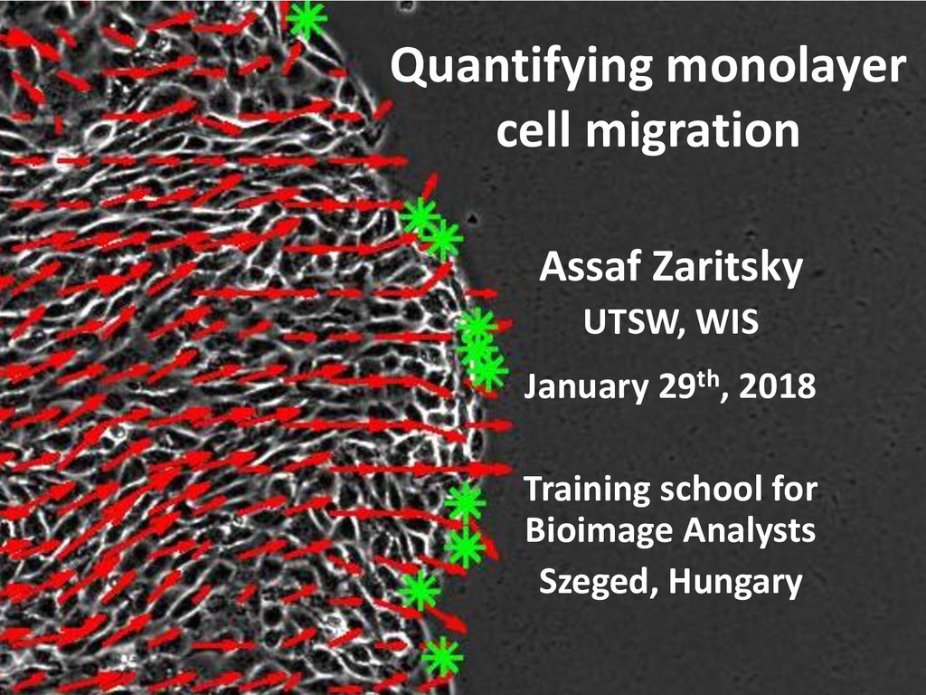
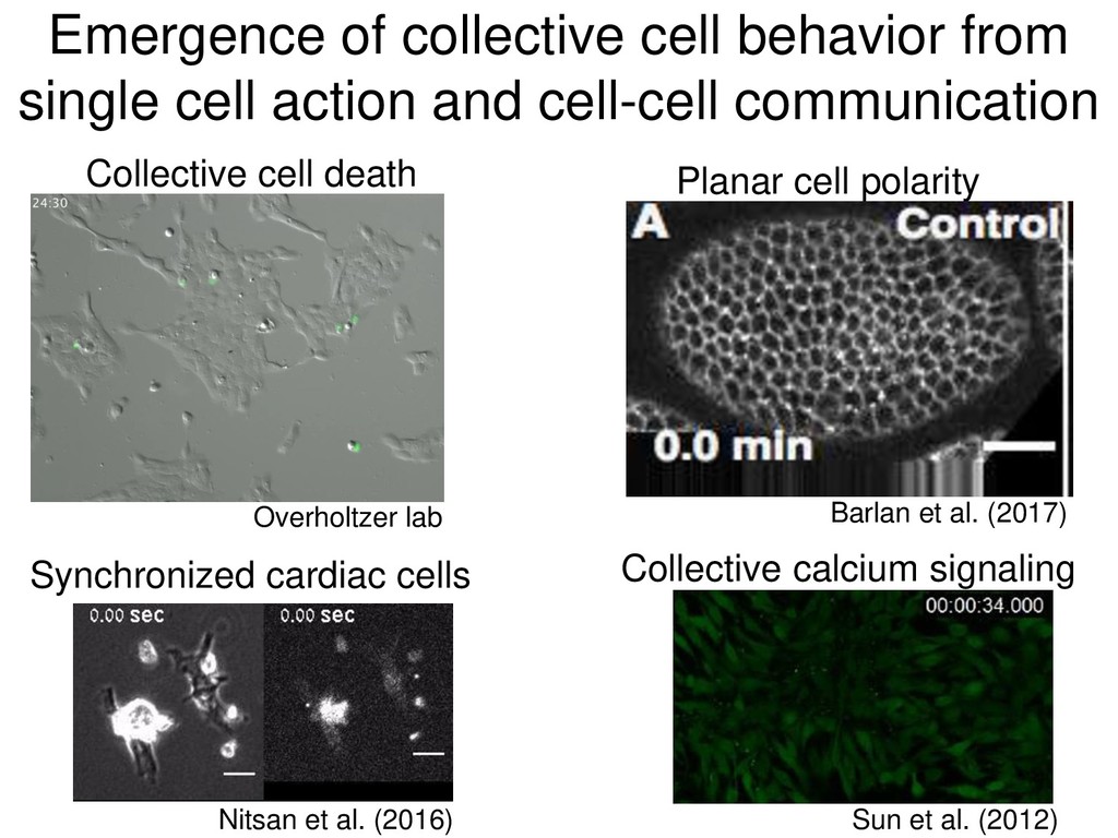
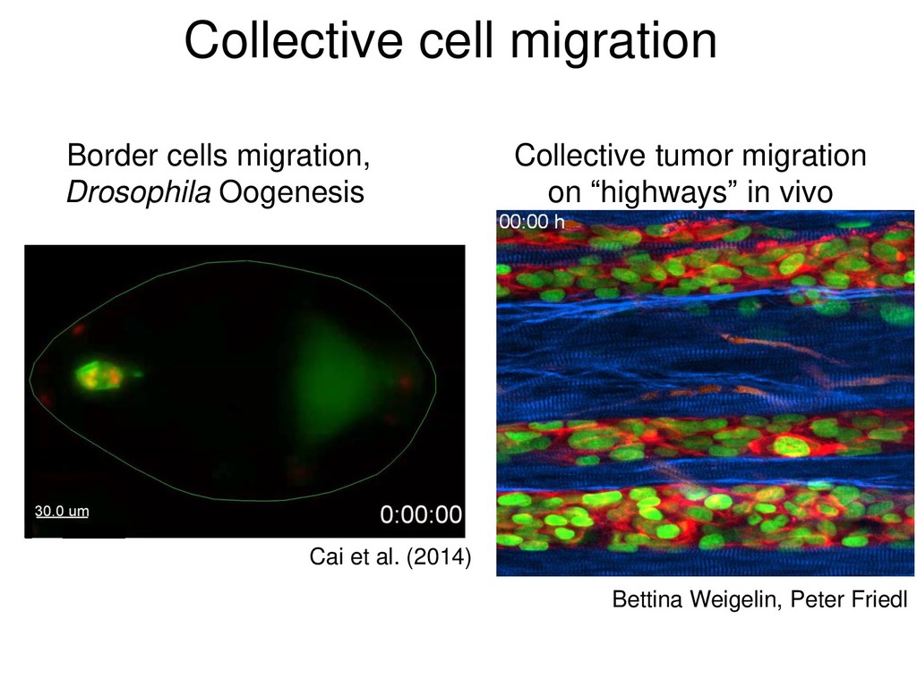
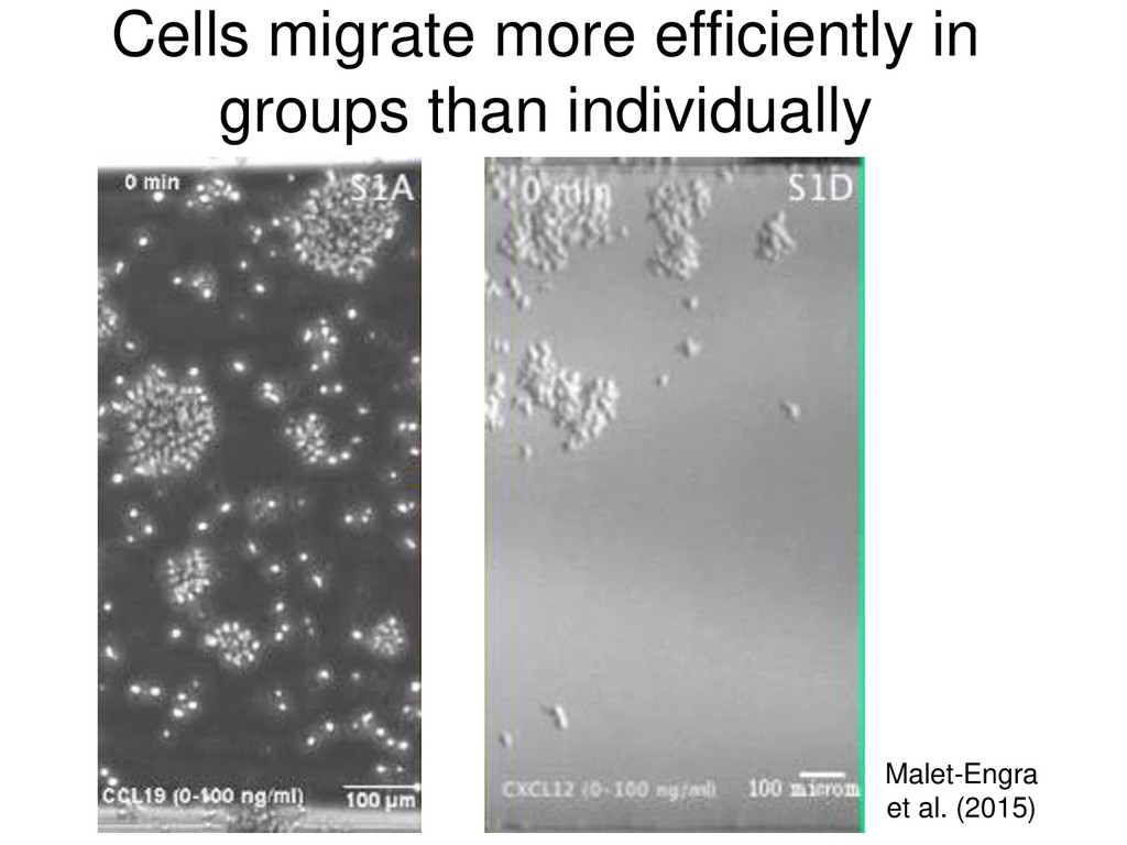
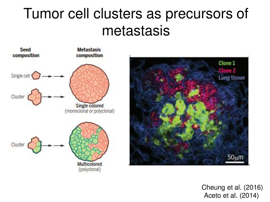
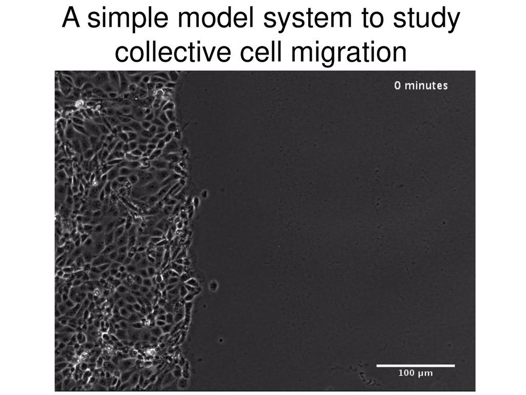
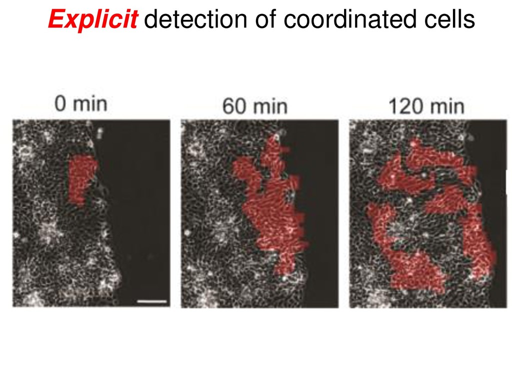
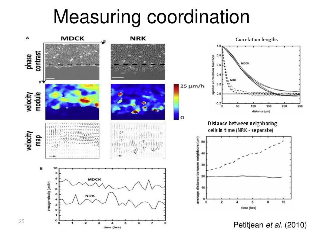
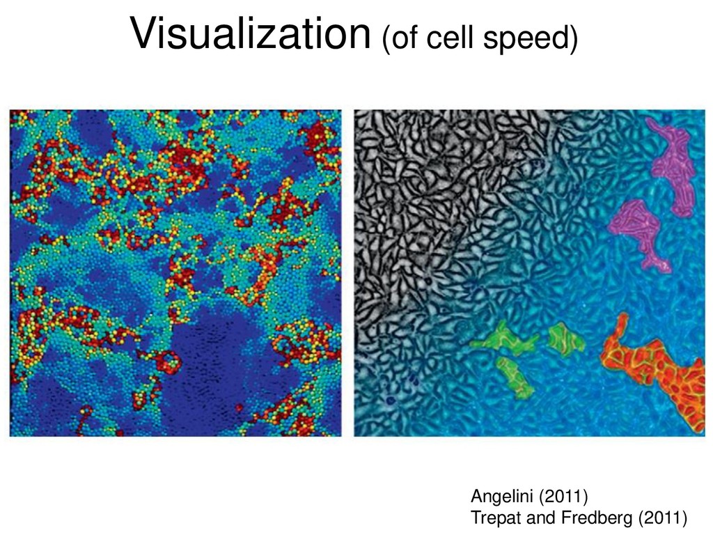
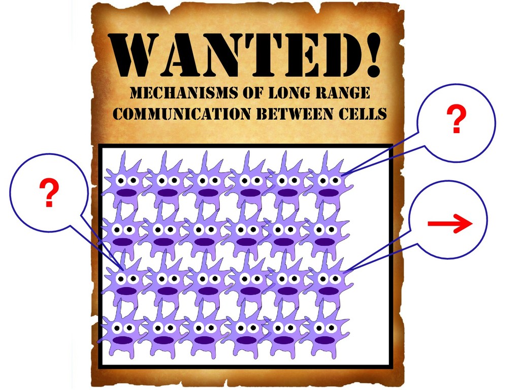
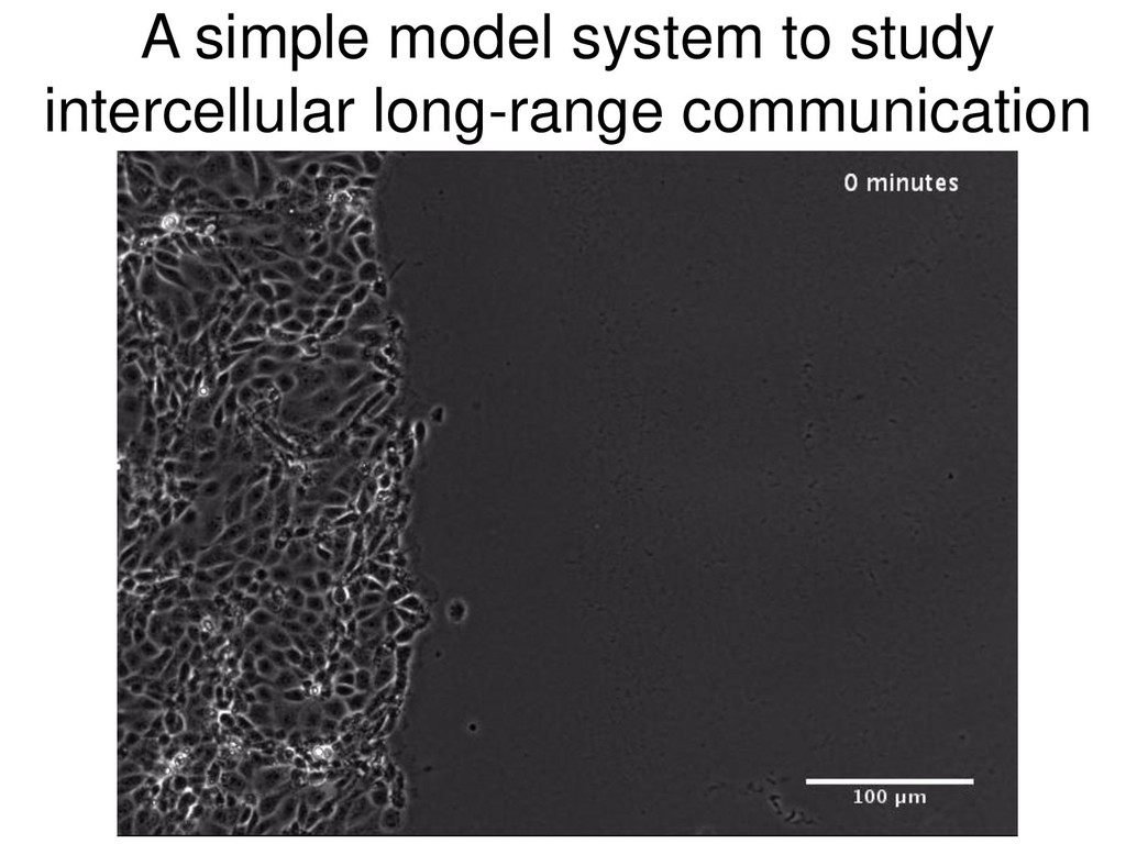
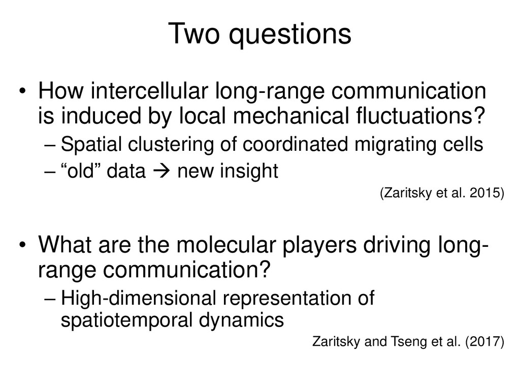
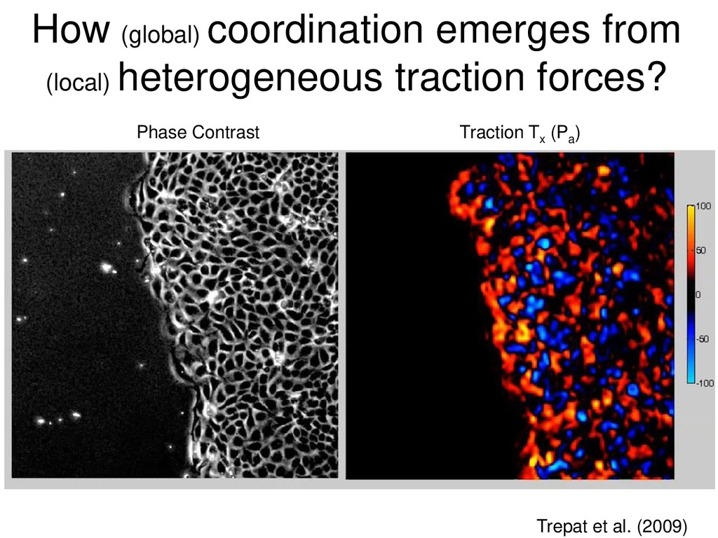
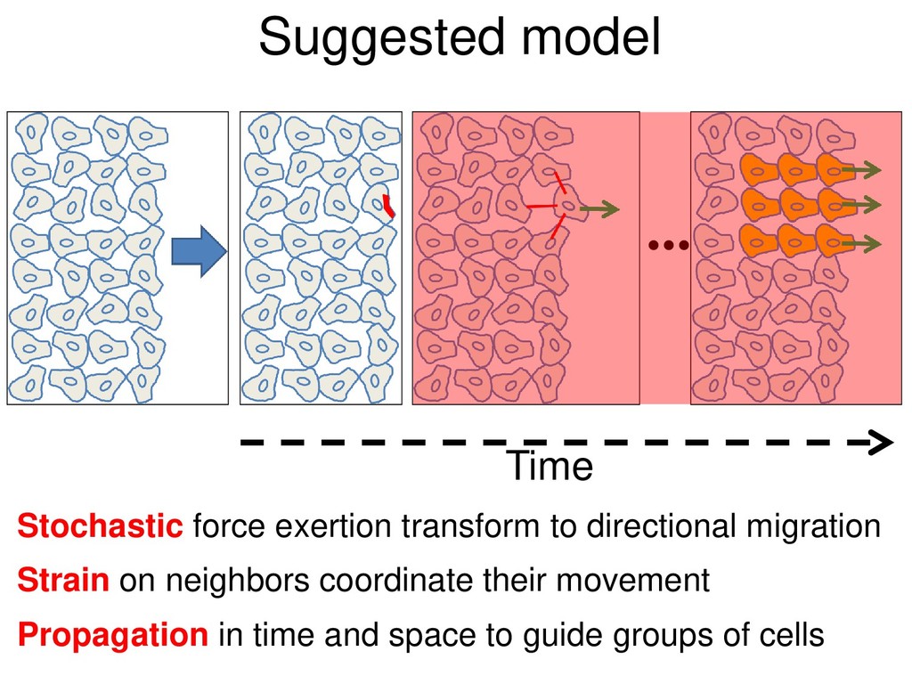
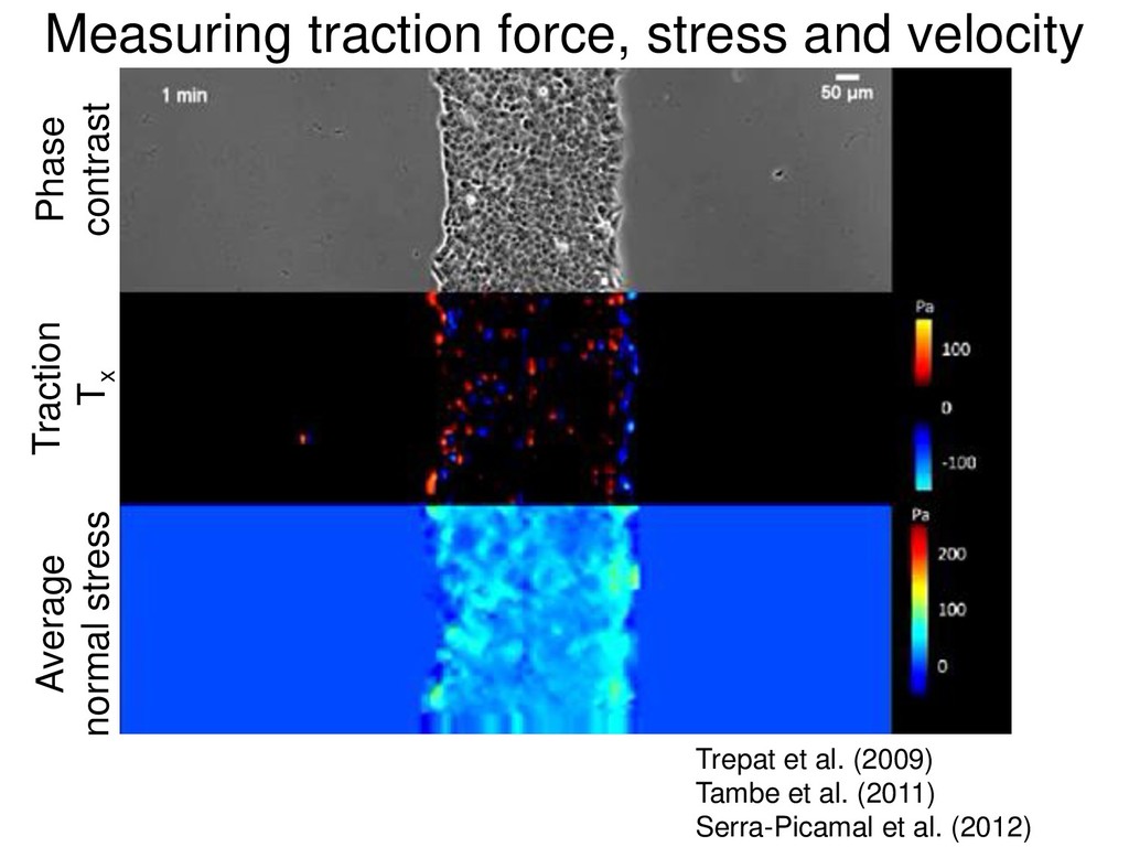
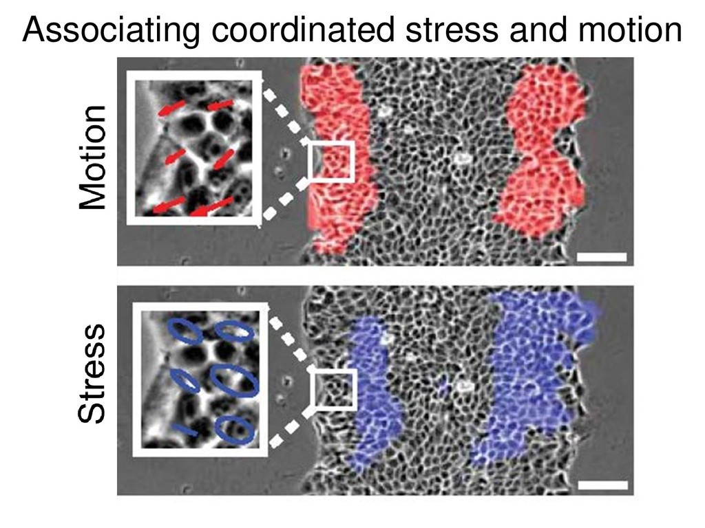
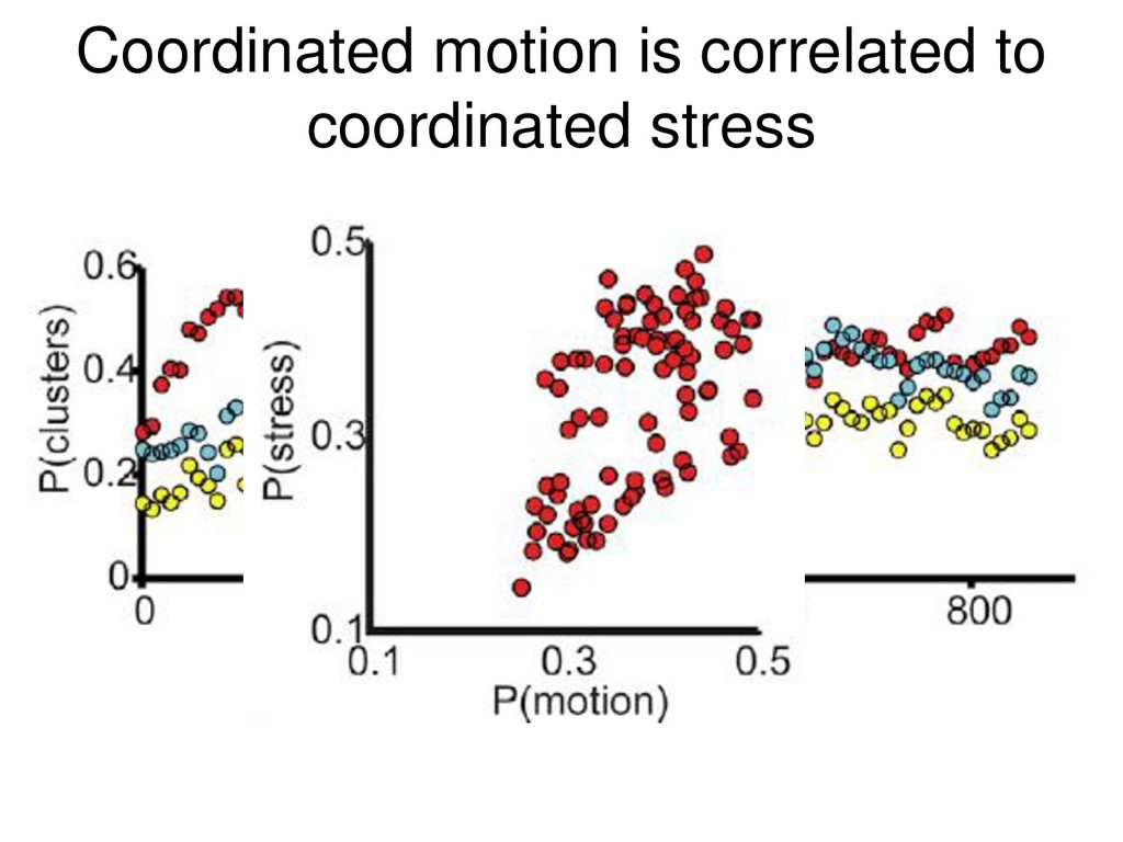
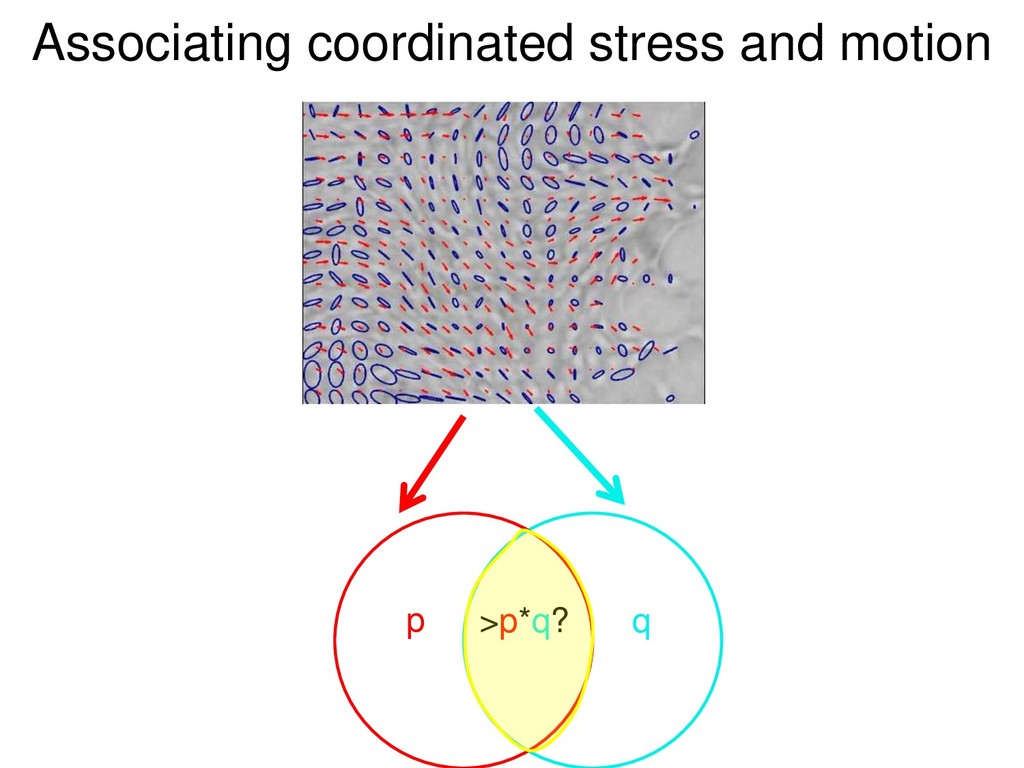
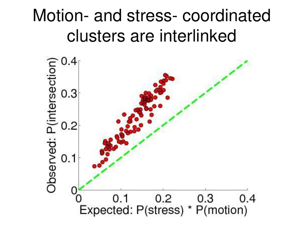
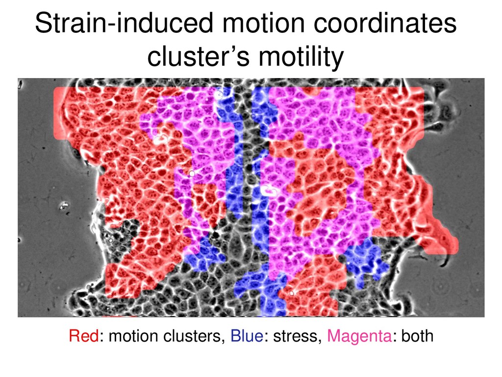
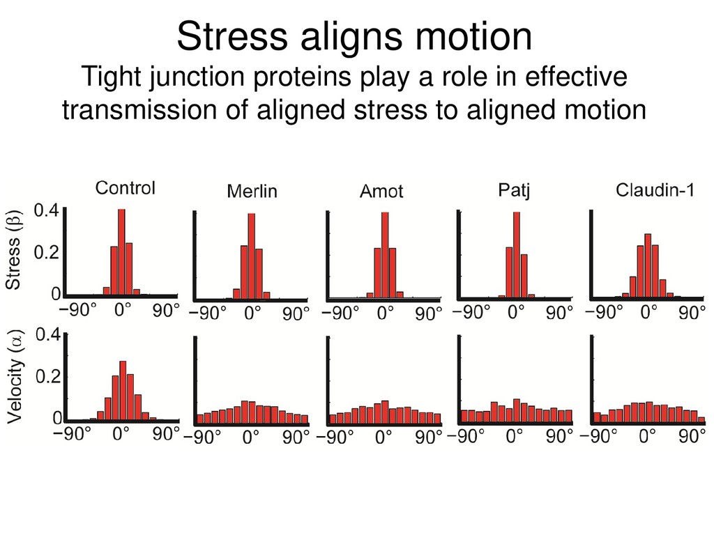
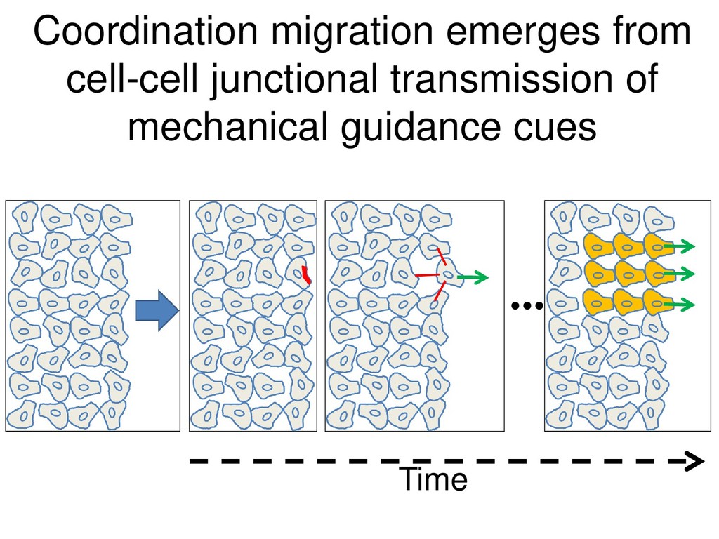
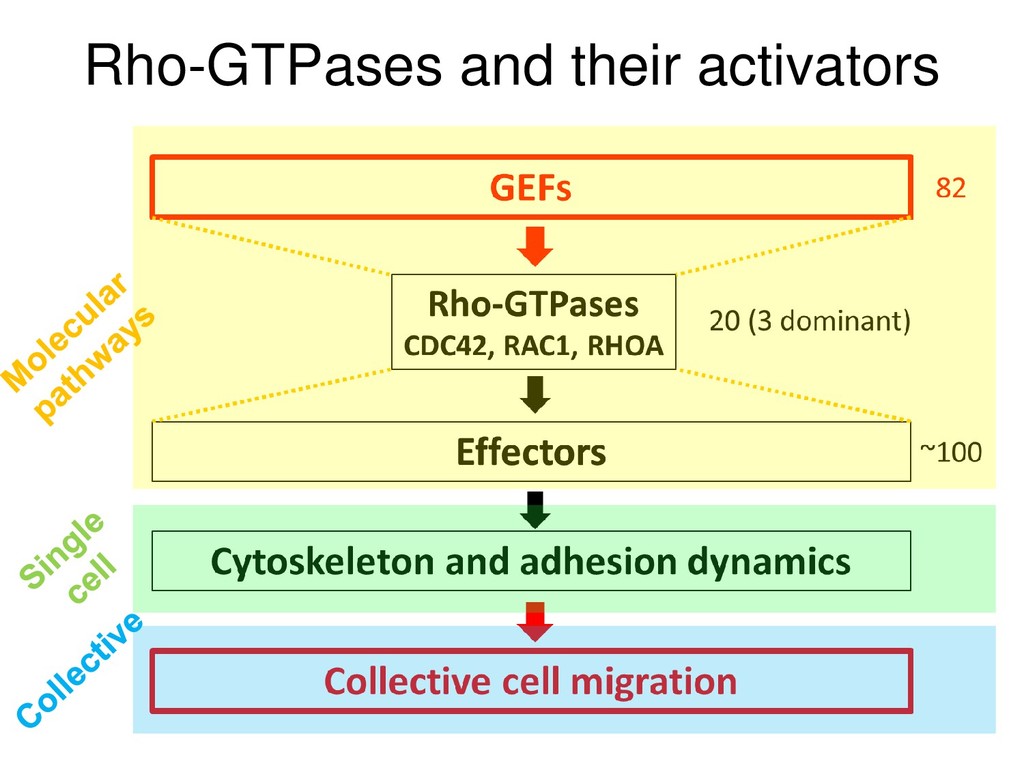
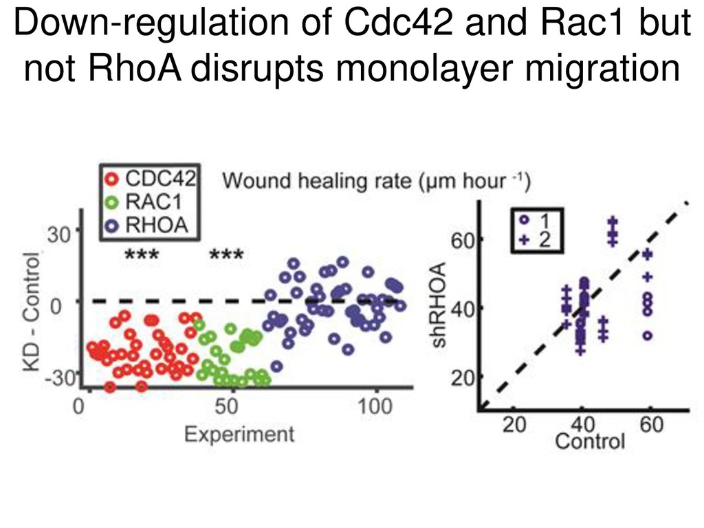
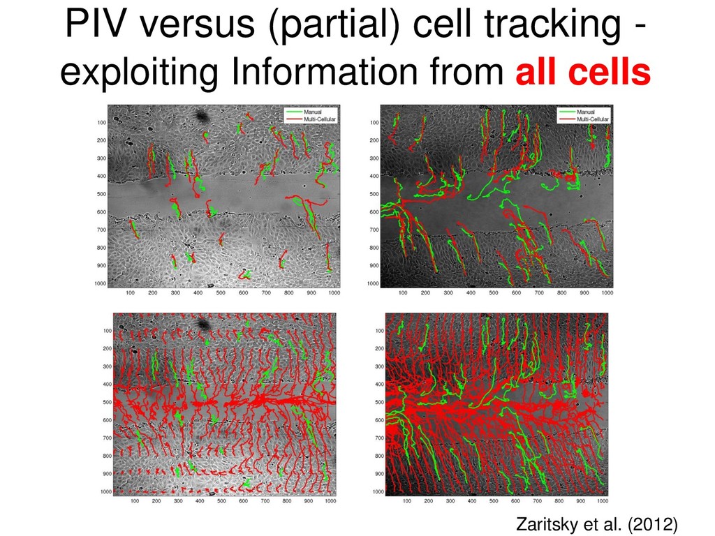
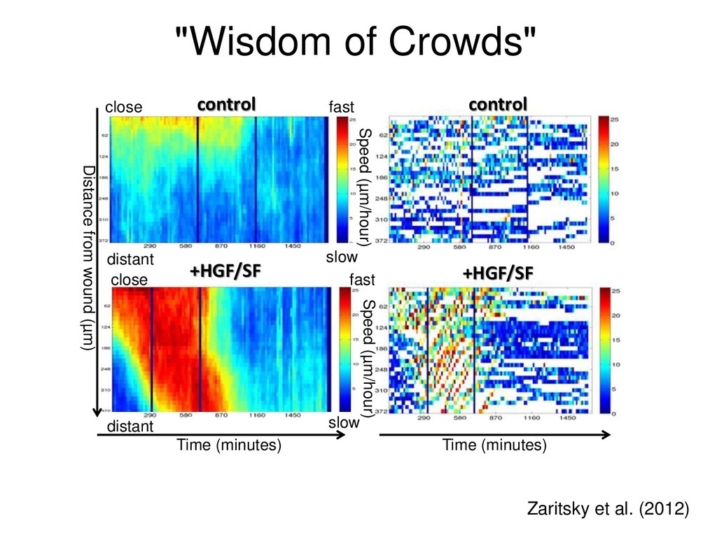
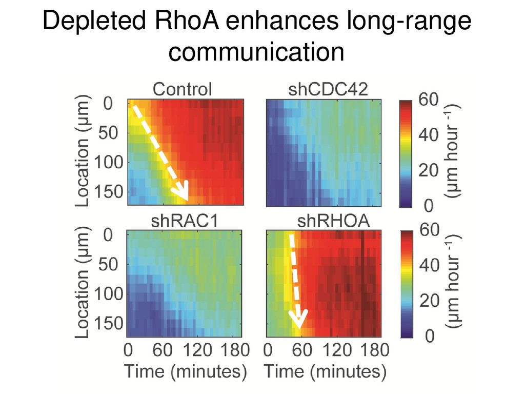
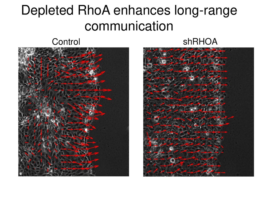
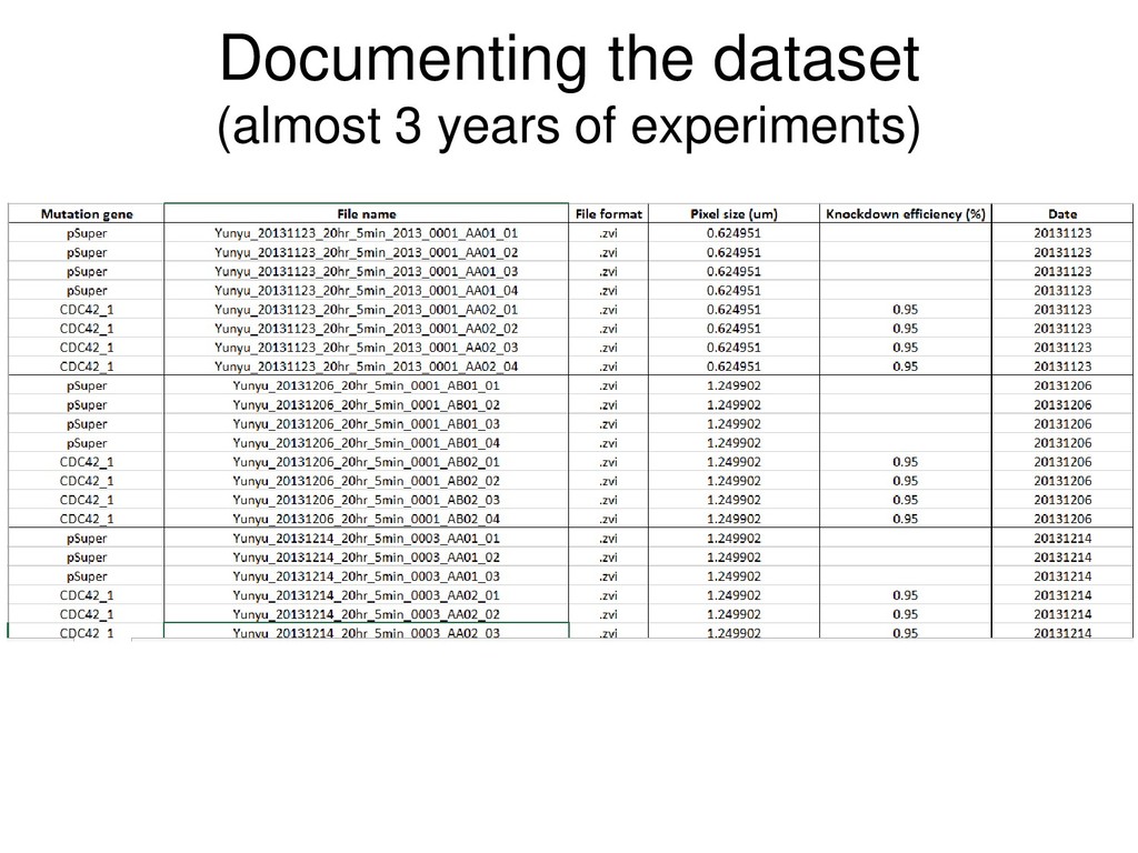
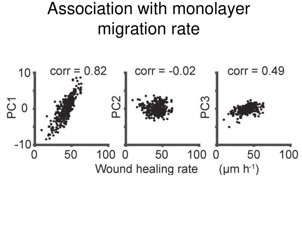
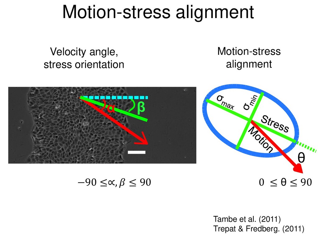
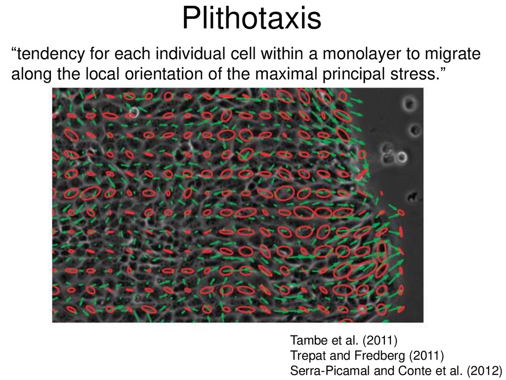
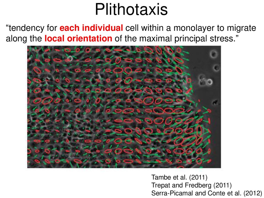
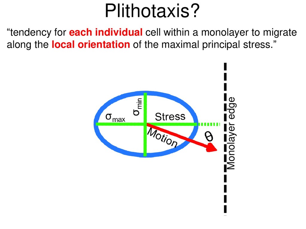
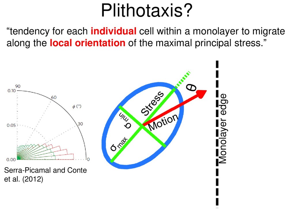
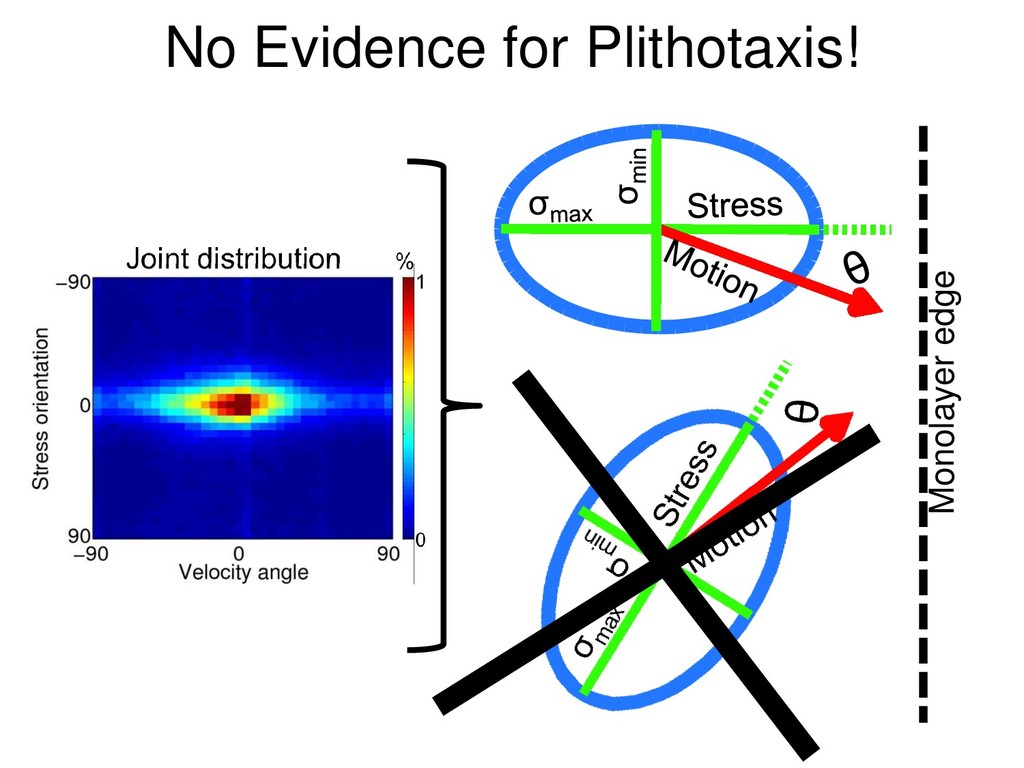
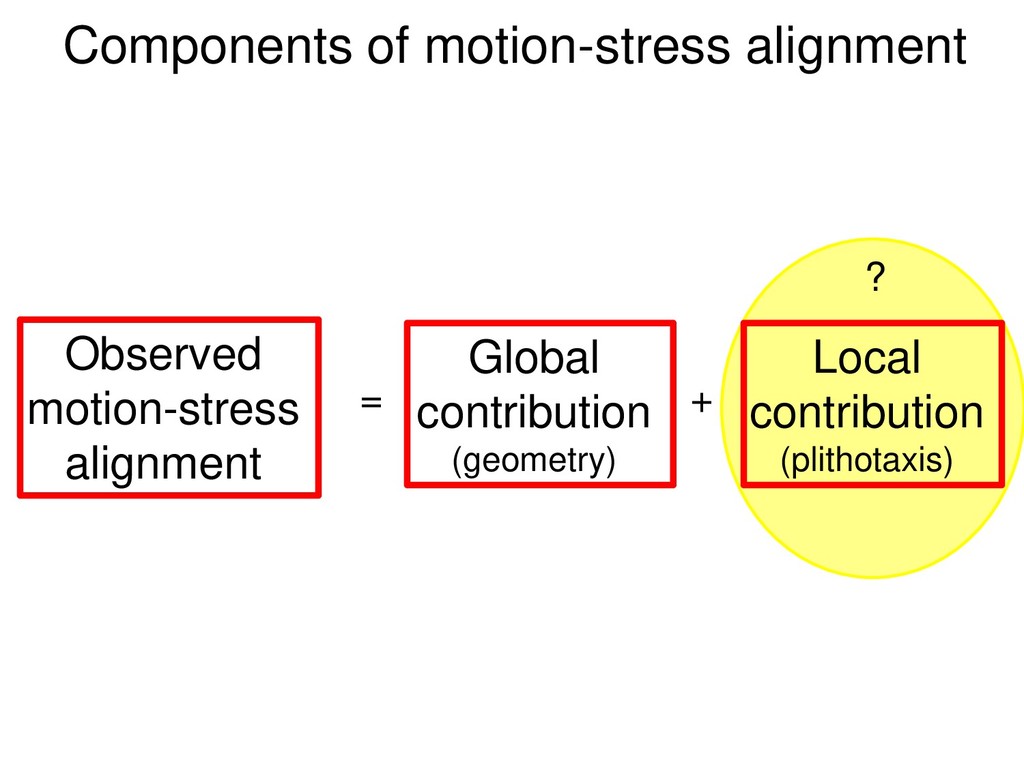
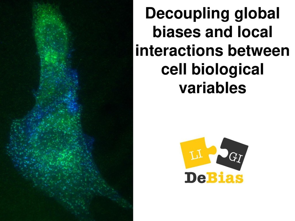
From embryonic development, through synchronized beating of cardiac muscle cells to collective cell death - individual cells use basic cellular machinery to influence and respond to neighboring cells through a complex interplay of chemical and physical cues. How these local interactions are integrated in space and time to induce collective patterns is yet unknown. By designing and applying new analytical methods to migrating monolayers of epithelial cells, we discovered how local mechanical fluctuations induce long-range inter-cellular communication and identified potential molecular pathways driving this communication.

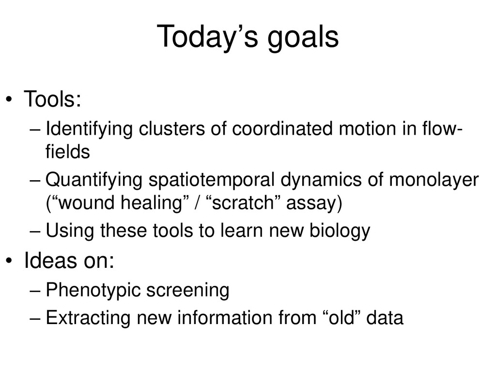
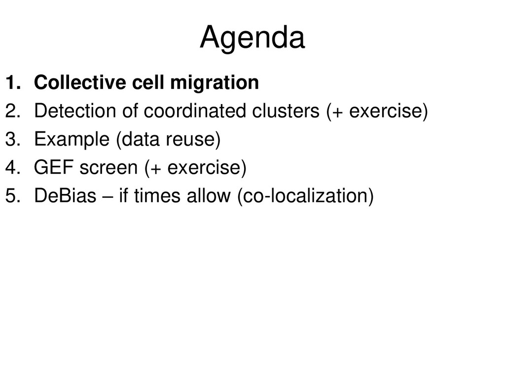
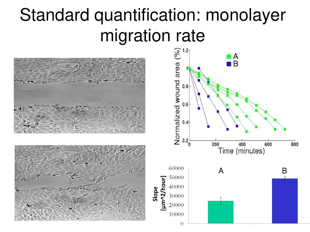
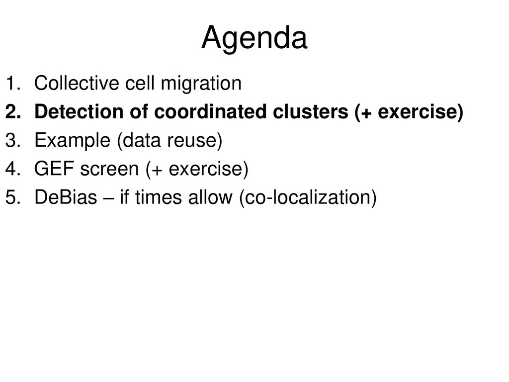
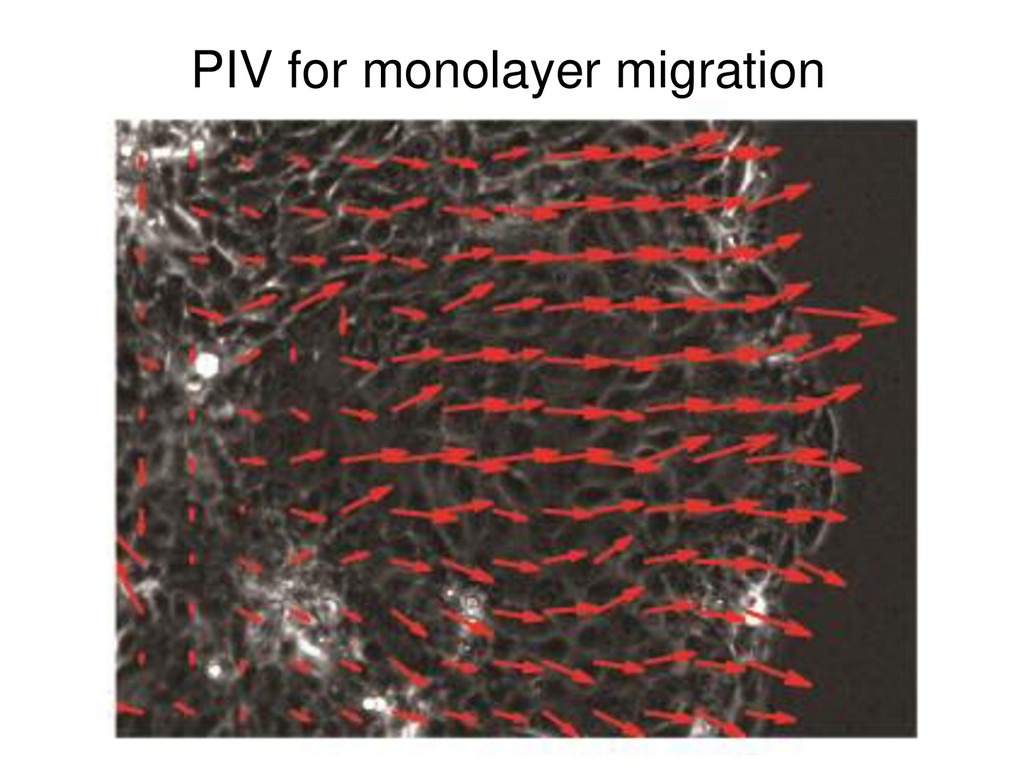
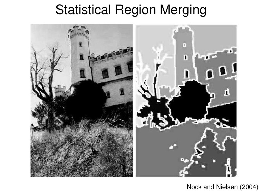
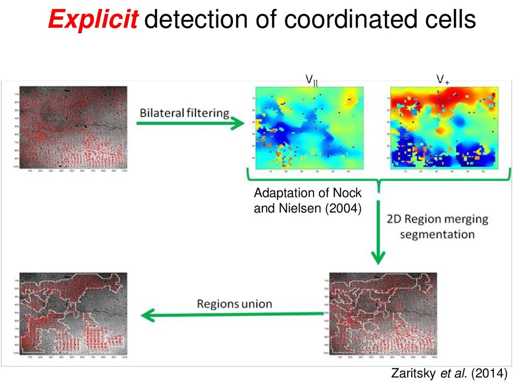
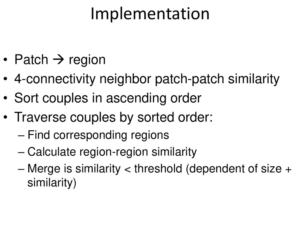
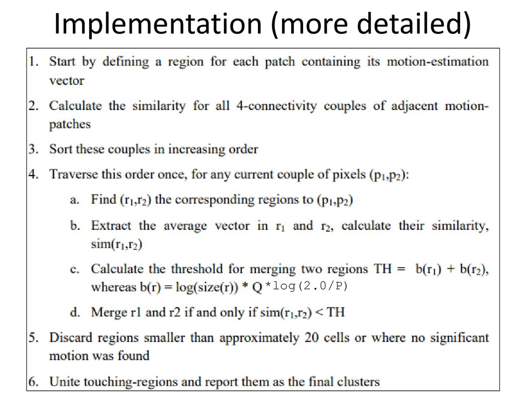
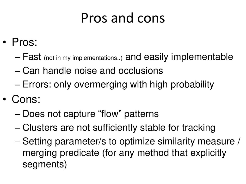
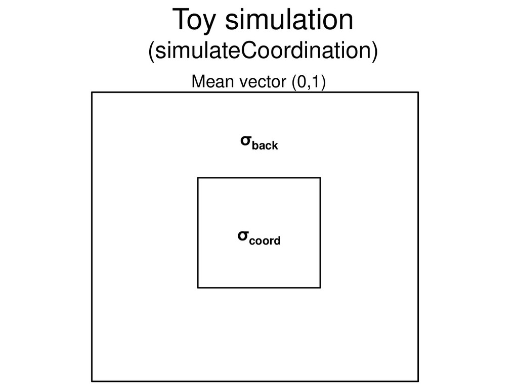
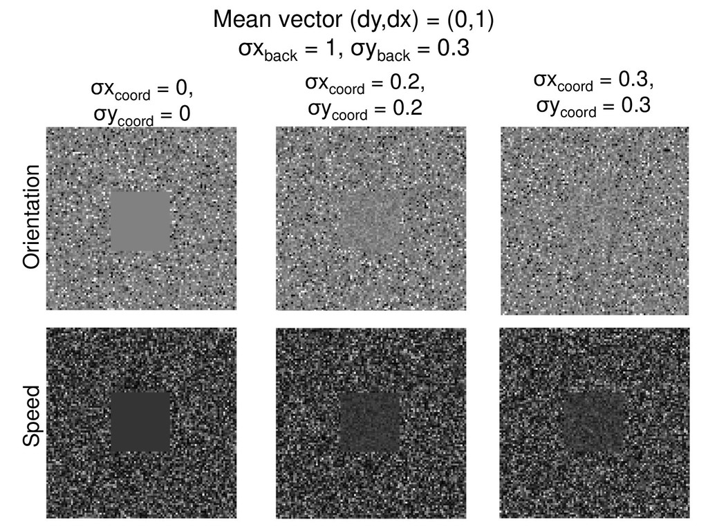
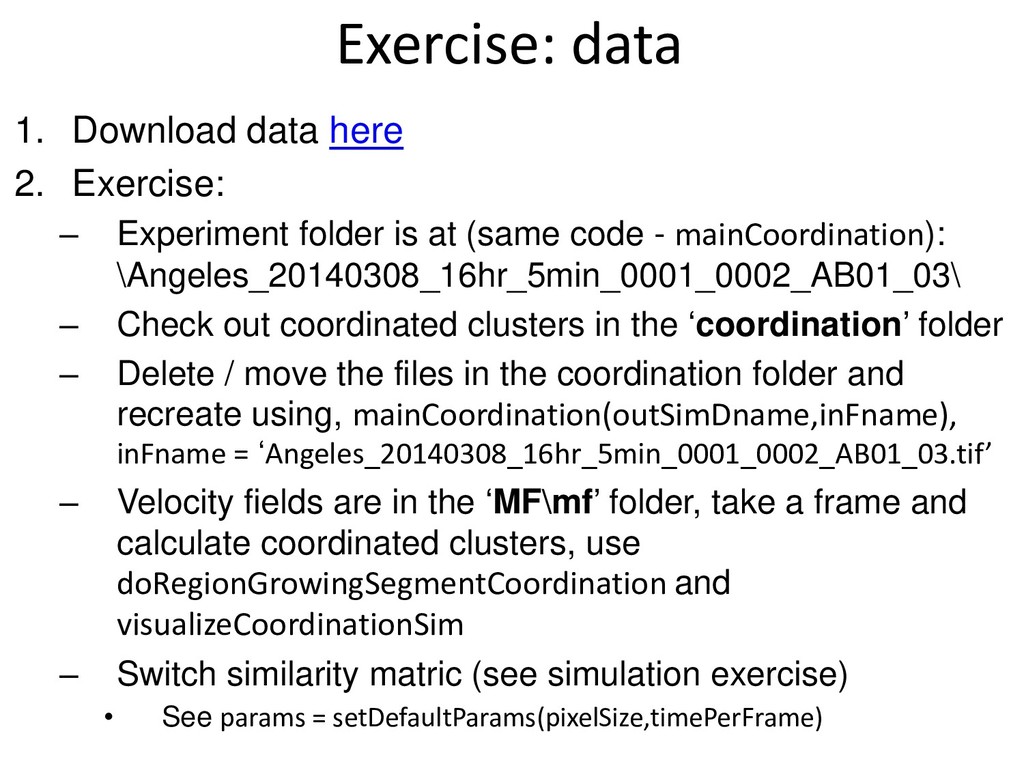
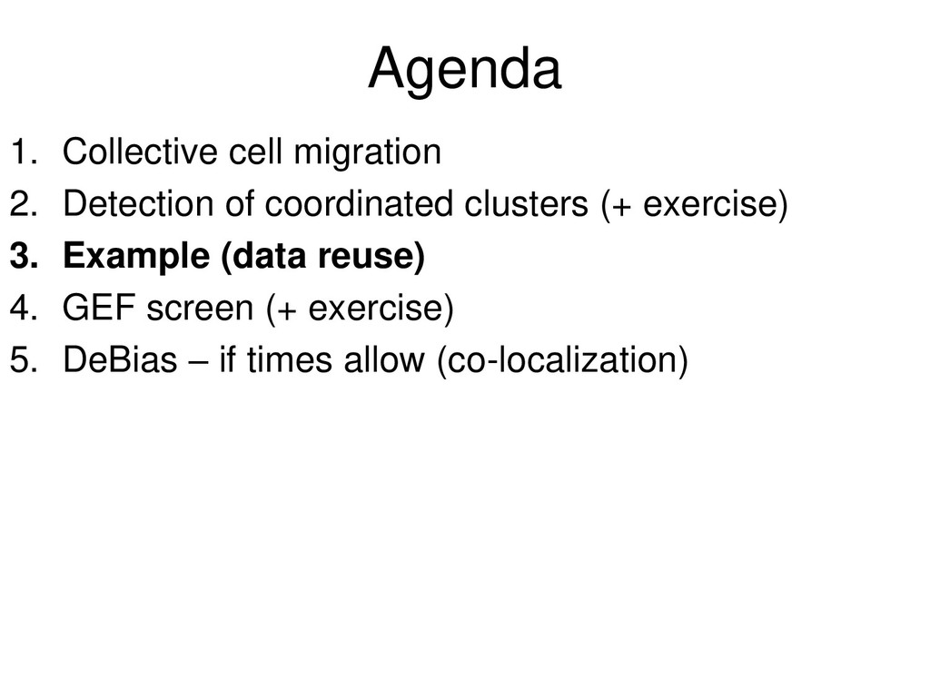
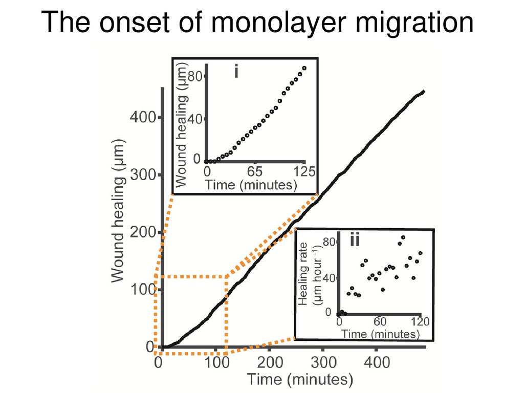
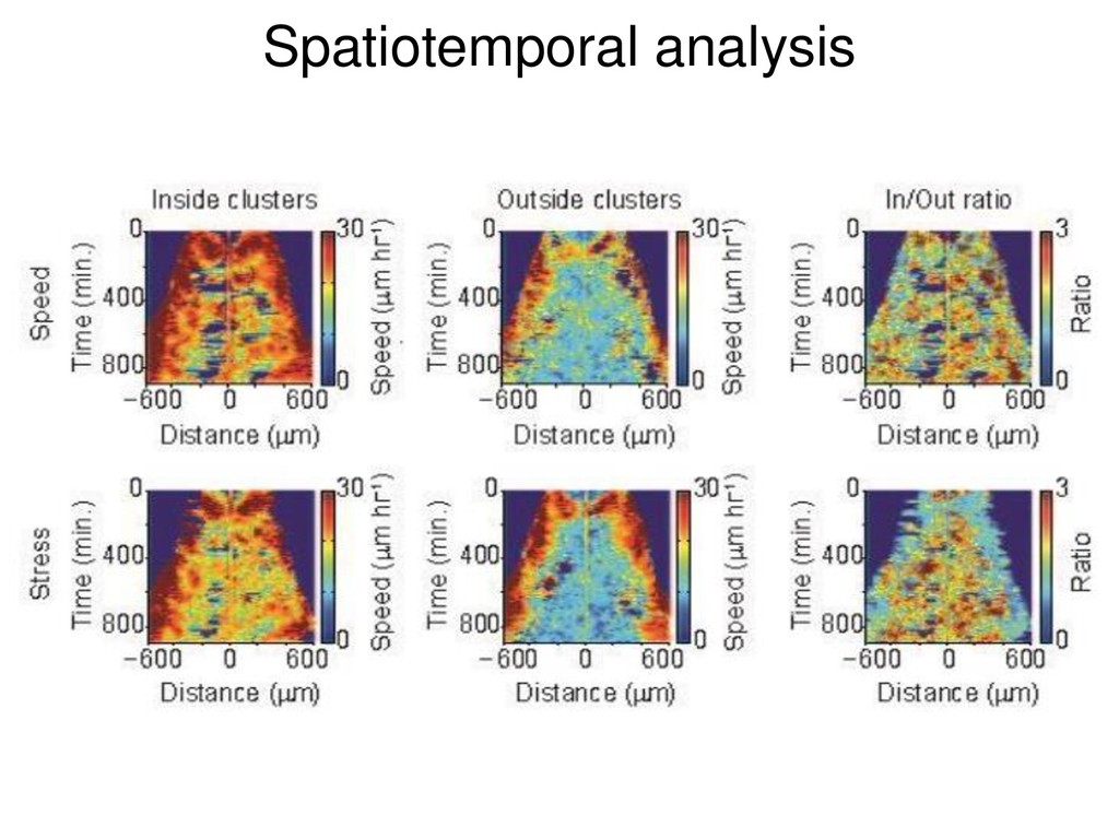
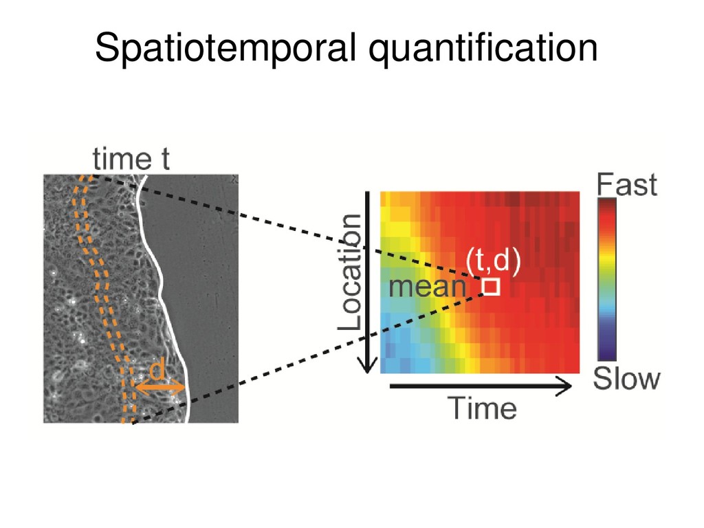
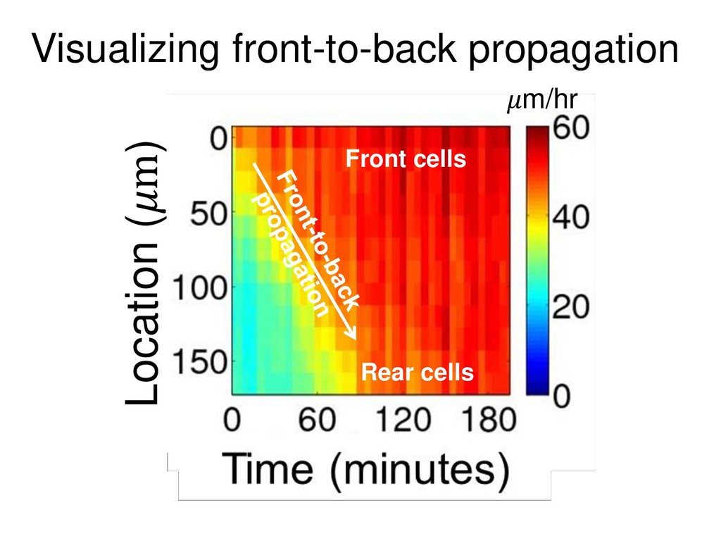
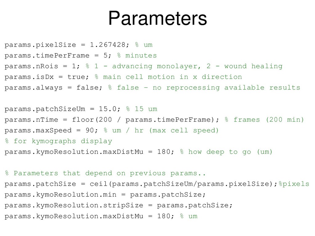
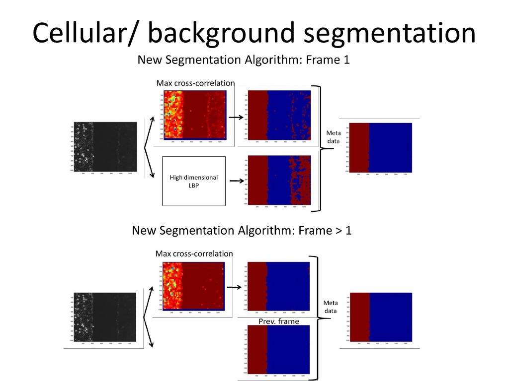
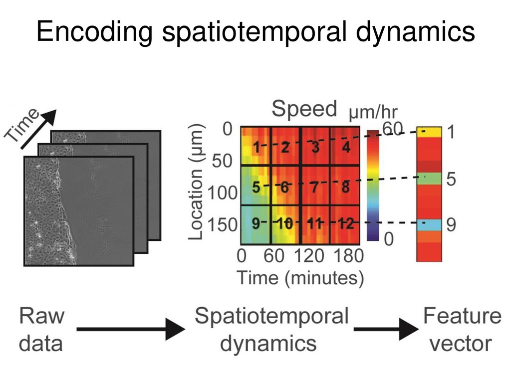
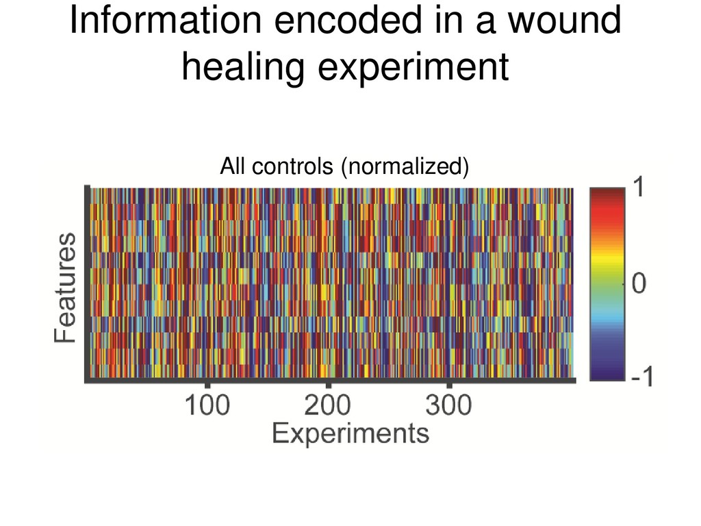
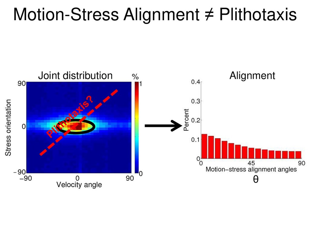
A key in advancing this project was the ability to quantify spatiotemporal dynamics of a migrating monolayer. In the workshop, we will demonstrate two such methods and discuss how they were applied to learn new biology: (1) Explicit segmention of coordinated migrating cell clusters; (2) Spatiotemporal representation of the onset of monolayer migration;

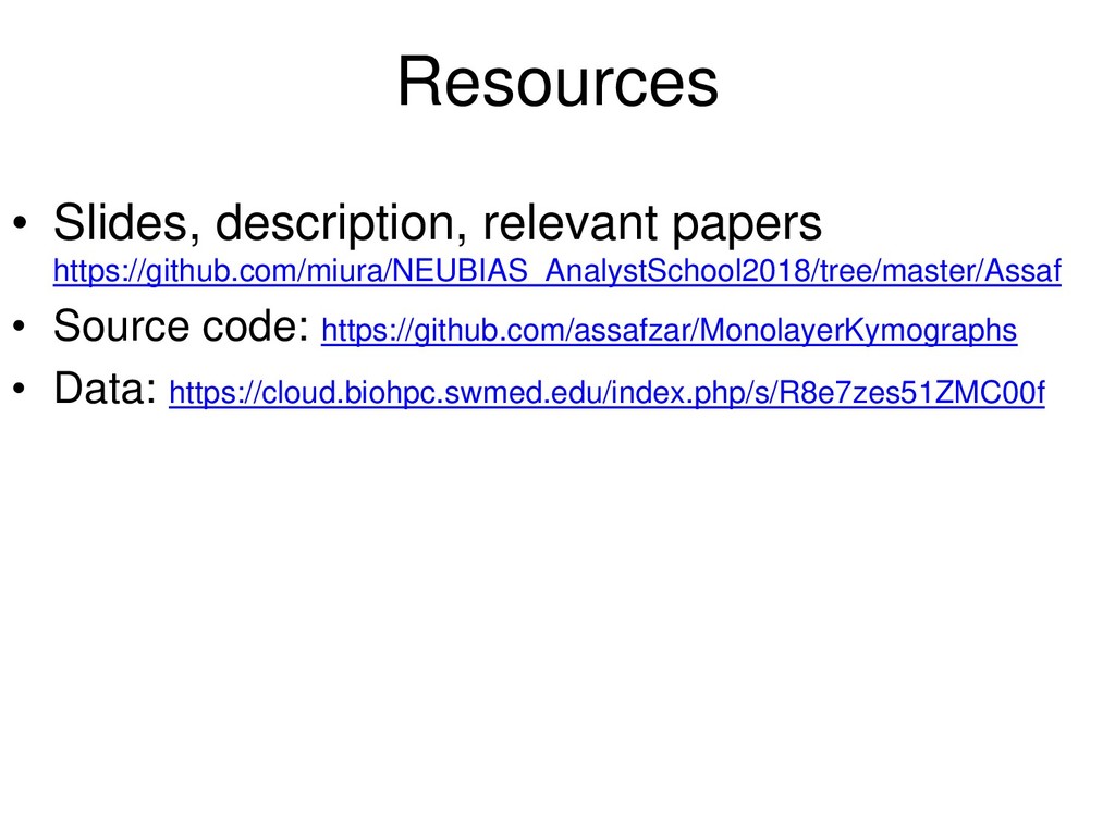
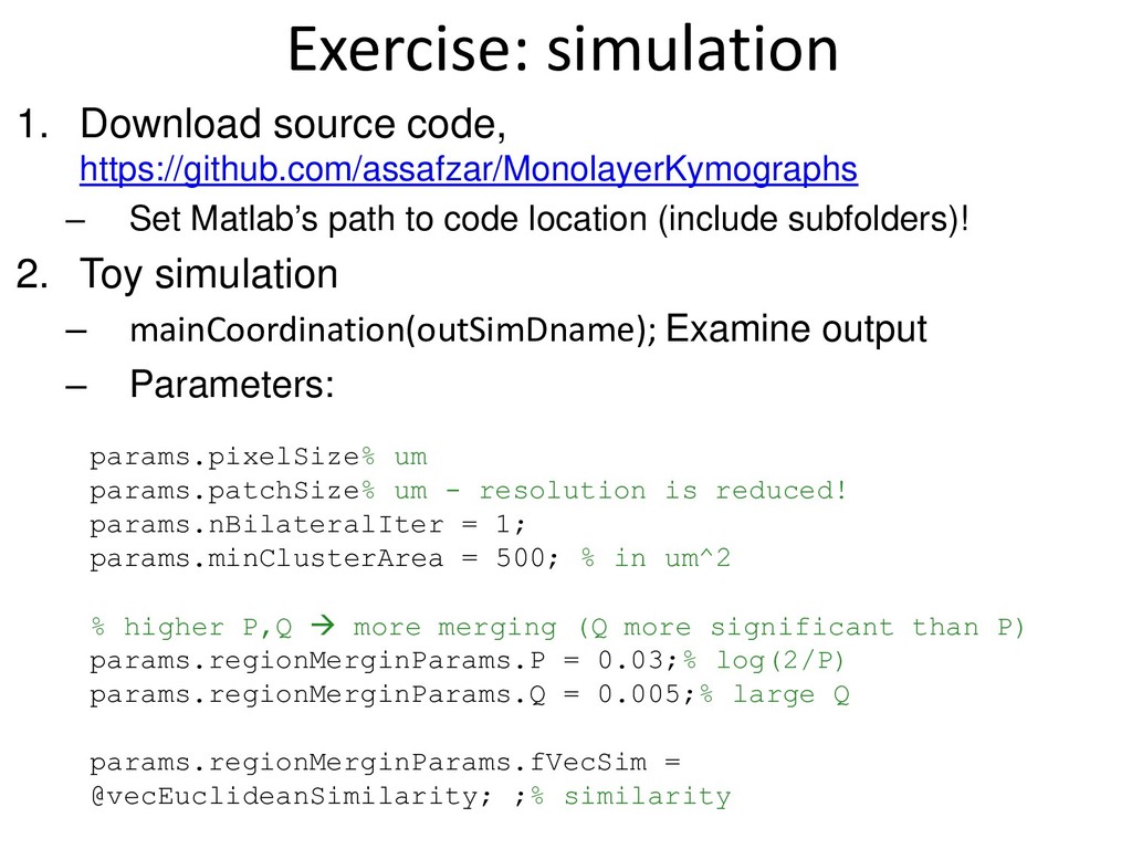
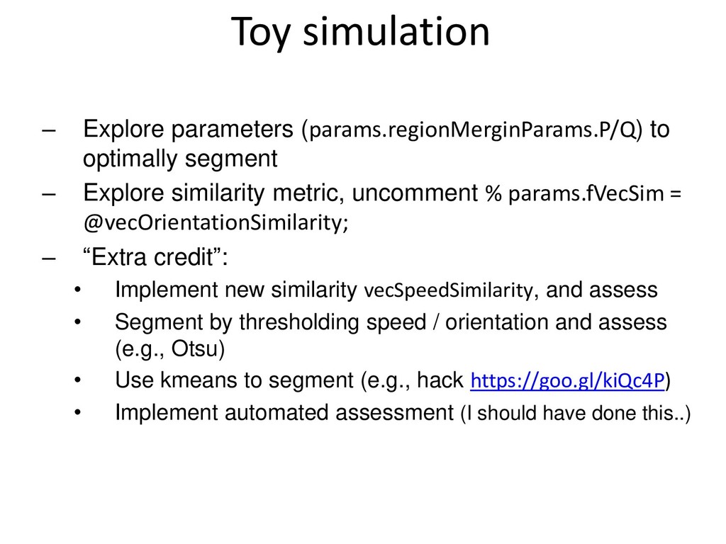
workshop material: https://github.com/miura/NEUBIAS_AnalystSchool2018/blob/master/Assaf/NEUBIAS_SzegedSchool_AssafZar.md

Transcript

1. Assaf Zaritsky UTSW, WIS January 29th, 2018 Training school for Bioimage Analysts Szeged, Hungary Quantifying monolayer cell migration
2. Today’s goals • Tools: – Identifying clusters of coordinated motion in flow- fields – Quantifying spatiotemporal dynamics of monolayer (“wound healing” / “scratch” assay) – Using these tools to learn new biology • Ideas on: – Phenotypic screening – Extracting new information from “old” data
3. Resources • Slides, description, relevant papers https://github.com/miura/NEUBIAS_AnalystSchool2018/tree/master/Assaf • Source code: https://github.com/assafzar/MonolayerKymographs • Data: https://cloud.biohpc.swmed.edu/index.php/s/R8e7zes51ZMC00f
4. Agenda 1. Collective cell migration 2. Detection of coordinated clusters (+ exercise) 3. Example (data reuse) 4. GEF screen (+ exercise) 5. DeBias – if times allow (co-localization)
5. Emergence of collective cell behavior from single cell action and cell-cell communication Collective cell death Planar cell polarity Overholtzer lab Nitsan et al. (2016) Synchronized cardiac cells Barlan et al. (2017) Sun et al. (2012) Collective calcium signaling
6. Collective cell migration Cai et al. (2014) Border cells migration, Drosophila Oogenesis Bettina Weigelin, Peter Friedl Collective tumor migration on “highways” in vivo
7. Cells migrate more efficiently in groups than individually Malet-Engra et al. (2015)
8. Tumor cell clusters as precursors of metastasis Cheung et al. (2016) Aceto et al. (2014)
9. A simple model system to study collective cell migration
10. A B B A Standard quantification: monolayer migration rate
11. Tools available Masuzzo et al. (2016)
12. Agenda 1. Collective cell migration 2. Detection of coordinated clusters (+ exercise) 3. Example (data reuse) 4. GEF screen (+ exercise) 5. DeBias – if times allow (co-localization)
13. Explicit detection of coordinated cells
14. Motivation Exploiting spatial heterogeneity to assess mechanisms of coordinated migration
15. Determining flow fields: Particle Image Velocimetry (PIV) Artwork: David Hellman (Braid); Adapted by Rachel Lee (U. Maryland)
16. Particle Image Velocimetry (PIV) Source: https://www.erc.wisc.edu/piv.php
17. PIV for monolayer migration
18. • Partial derivatives with respect to the spatial and temporal coordinates • Lucas–Kanade method • Assumptions: • motion is small • smooth change • Fast • Many extensions (gradient based) optical flow Lucas & Kanade (1981)
19. Optical flow versus PIV Vig et al. (2016)
20. Measuring coordination 25 25 Petitjean et al. (2010)
21. Visualization (of cell speed) Angelini (2011) Trepat and Fredberg (2011)
22. Statistical Region Merging Nock and Nielsen (2004)
23. Region growing / merging • Regions: sets of pixels with homogeneous properties • Iteratively combining smaller regions (“growing”) • Statistical test to decide whether to merge or not • Balances sustainment of perceptual units vs. over- merging • Here: implementation for velocity fields
24. Algorithmic components • Initialization • Metric for region similarity • Merging predicate • Merging order (greedy)
25. Explicit detection of coordinated cells Zaritsky et al. (2014) Adaptation of Nock and Nielsen (2004)
26. Implementation • Patch  region • 4-connectivity neighbor patch-patch similarity • Sort couples in ascending order • Traverse couples by sorted order: – Find corresponding regions – Calculate region-region similarity – Merge is similarity < threshold (dependent of size + similarity)
27. Implementation (more detailed) *log(2.0/P)
28. Pros and cons • Pros: – Fast (not in my implementations..) and easily implementable – Can handle noise and occlusions – Errors: only overmerging with high probability • Cons: – Does not capture “flow” patterns – Clusters are not sufficiently stable for tracking – Setting parameter/s to optimize similarity measure / merging predicate (for any method that explicitly segments)
29. Toy simulation (simulateCoordination) Mean vector (0,1) σcoord σback
30. Mean vector (dy,dx) = (0,1) σxback = 1, σyback = 0.3 σxcoord = 0, σycoord = 0 Orientation Speed σxcoord = 0.2, σycoord = 0.2 σxcoord = 0.3, σycoord = 0.3
31. Exercise: simulation 1. Download source code, https://github.com/assafzar/MonolayerKymographs – Set Matlab’s path to code location (include subfolders)! 2. Toy simulation – mainCoordination(outSimDname); Examine output – Parameters: params.pixelSize% um params.patchSize% um - resolution is reduced! params.nBilateralIter = 1; params.minClusterArea = 500; % in um^2 % higher P,Q  more merging (Q more significant than P) params.regionMerginParams.P = 0.03;% log(2/P) params.regionMerginParams.Q = 0.005;% large Q params.regionMerginParams.fVecSim = @vecEuclideanSimilarity; ;% similarity
32. Toy simulation – Explore parameters (params.regionMerginParams.P/Q) to optimally segment – Explore similarity metric, uncomment % params.fVecSim = @vecOrientationSimilarity; – “Extra credit”: • Implement new similarity vecSpeedSimilarity, and assess • Segment by thresholding speed / orientation and assess (e.g., Otsu) • Use kmeans to segment (e.g., hack https://goo.gl/kiQc4P) • Implement automated assessment (I should have done this..)
33. Exercise: data 1. Download data here 2. Exercise: – Experiment folder is at (same code - mainCoordination): \Angeles_20140308_16hr_5min_0001_0002_AB01_03\ – Check out coordinated clusters in the ‘coordination’ folder – Delete / move the files in the coordination folder and recreate using, mainCoordination(outSimDname,inFname), inFname = ‘Angeles_20140308_16hr_5min_0001_0002_AB01_03.tif’ – Velocity fields are in the ‘MF\mf’ folder, take a frame and calculate coordinated clusters, use doRegionGrowingSegmentCoordination and visualizeCoordinationSim – Switch similarity matric (see simulation exercise) • See params = setDefaultParams(pixelSize,timePerFrame)
34. Agenda 1. Collective cell migration 2. Detection of coordinated clusters (+ exercise) 3. Example (data reuse) 4. GEF screen (+ exercise) 5. DeBias – if times allow (co-localization)
35. mechanisms of long range communication between cells WANTED! ? ?
36. A simple model system to study intercellular long-range communication
37. The onset of monolayer migration
38. Two questions • How intercellular long-range communication is induced by local mechanical fluctuations? – Spatial clustering of coordinated migrating cells – “old” data  new insight (Zaritsky et al. 2015) • What are the molecular players driving long- range communication? – High-dimensional representation of spatiotemporal dynamics Zaritsky and Tseng et al. (2017)
39. Trepat et al. (2009) How (global) coordination emerges from (local) heterogeneous traction forces? Traction Tx (Pa ) Phase Contrast
40. Suggested model Time Stochastic force exertion transform to directional migration Strain on neighbors coordinate their movement Propagation in time and space to guide groups of cells
41. Measuring traction force, stress and velocity Phase contrast Traction Tx Average normal stress Trepat et al. (2009) Tambe et al. (2011) Serra-Picamal et al. (2012)
42. Motion-stress alignment Tambe et al. (2011) Trepat & Fredberg. (2011) β −90 ≤∝, ≤ 90 Velocity angle, stress orientation θ 0 ≤ θ ≤ 90 Motion-stress alignment α
43. Region-growing segmentation for explicit detection of coordinated migration clusters
44. Associating coordinated stress and motion
45. Coordinated motion is correlated to coordinated stress
46. q p >p*q? Associating coordinated stress and motion
47. Motion- and stress- coordinated clusters are interlinked
48. Cells in coordinated clusters move faster, with enhanced motion-stress alignment Ratioproperty = propertyin propertyout
49. Spatiotemporal analysis
50. Strain-induced motion coordinates cluster’s motility Red: motion clusters, Blue: stress, Magenta: both
51. Strain-induced motion coordinates cluster’s motility Red: motion clusters, Blue: stress Fraction of coordinated cells
52. Stress aligns motion Tight junction proteins play a role in effective transmission of aligned stress to aligned motion
53. Coordination migration emerges from cell-cell junctional transmission of mechanical guidance cues Time
54. Identifying coordinated clusters of velocities can be also useful in other cortexes - discussion
55. Agenda 1. Collective cell migration 2. Detection of coordinated clusters (+ exercise) 3. Example (data reuse) 4. GEF screen (+ exercise) 5. DeBias – if times allow (co-localization)
56. Rho-GTPases and their activators
57. Down-regulation of Cdc42 and Rac1 but not RhoA disrupts monolayer migration
58. Spatiotemporal quantification Front cells Rear cells
59. Visualizing front-to-back propagation Front cells Rear cells m/hr Location (m)
60. Workflow processTimeLapse(filename,params); [params,dirs] = initParamsDirs(filename,params); % set missing parameters, create output directories whLocalMotionEstimation(params,dirs); % velocity fields estimation whTemporalBasedSegmentation(params,dirs); % cellular- background segmentation whCorrectGlobalMotion(params,dirs); % correction of stage-location errors whSegmentationMovie(params,dirs); % segmentation movie whHealingRate(params,dirs); % wound healing rate over time whCoordination(params,dirs); % coordinated clusters whKymographs(params,dirs); % spatiotemporal kymographs
61. Parameters params.pixelSize = 1.267428; % um params.timePerFrame = 5; % minutes params.nRois = 1; % 1 - advancing monolayer, 2 - wound healing params.isDx = true; % main cell motion in x direction params.always = false; % false – no reprocessing available results params.patchSizeUm = 15.0; % 15 um params.nTime = floor(200 / params.timePerFrame); % frames (200 min) params.maxSpeed = 90; % um / hr (max cell speed) % for kymographs display params.kymoResolution.maxDistMu = 180; % how deep to go (um) % Parameters that depend on previous params.. params.patchSize = ceil(params.patchSizeUm/params.pixelSize);%pixels params.kymoResolution.min = params.patchSize; params.kymoResolution.stripSize = params.patchSize; params.kymoResolution.maxDistMu = 180; % um
62. Two side notes 1. Segmentation 2. Flow fields vs. single cell tracking
63. Cellular/ background segmentation
64. Zaritsky et al. (2012) PIV versus (partial) cell tracking - exploiting Information from all cells
65. " Wisdom of Crowds " Time (minutes) slow fast slow control close distant Distance from wound (µm) close distant +HGF/SF Time (minutes) control Speed (µm/hour) Speed (µm/hour) +HGF/SF Zaritsky et al. (2012) fast
66. Depleted RhoA enhances long-range communication
67. Control shRHOA Depleted RhoA enhances long-range communication
68. Comprehensive GEFs screen • 81 GEFs, 3 (validated) hairpins, > 3 locations per condition • Control and follow-up experiments • > 3,000 videos to analyze • Robust algorithmic pipeline • Variability • Measures for screening
69. Comprehensive GEFs screen
70. Documenting the dataset (almost 3 years of experiments)
71. Encoding spatiotemporal dynamics
72. Information encoded in a wound healing experiment All controls (normalized)
73. Association with monolayer migration rate
74. Reverse engineering: what information is encoded in an experiment?
75. Effect on PCs by depletion of canonical Rho GTPAses Masking
76. Measures
77. Screening methodology
78. Knockdown efficiencies
79. Inter-day variability in controls • 6 well plates • 3 shRNAs + 1 control (pSuper) • 4-6 locations imaged per well sh1 sh2 sh3 pSuper
80. Scoring a knockdown phenotype Dunn index, Davies-Bouldin index, silhouette coefficient
81. Quantifying off-target effects • Exploiting 0% KD Experiments & “Known” Targets – 0% KD as off-target controls – CDC42, RAC1, β-PIX as positive controls FP FN “HITS”
82. Screen
83. Screen hits
84. Screen hits - visualization
85. Validation (and discovering new phenotypes)
86. Greatest hits RhoA GEFs inhibit long-range communication
87. What about Myosin? Kevin Dean, @kD3AN
88. Downstream effectors of RhoA
89. Actomyosin contractility disturbs intercellular communication downstream of the ARHGEF18 - RHOA pathway
90. Differential functional roles of RhoA-GEFs down-stream of RhoA signaling Contractility inhibition
91. Rho isoforms are required for collective migration You will reproduce (part of) this figure as exercise
92. RhoC has an intermediate phenotype
93. Diverse roles of GEFs in regulating collective cell migration
94. RhoA-GEFs/RhoA/Myosin-II balances motile forces vs. mechanical guidance generation of motile forces transmission of guidance cues
95. References, resources References: – Zaritsky et al. Propagating waves of directionality and coordination orchestrate collective cell migration (2014) http://journals.plos.org/ploscompbiol/article?id=10.1371/journal. pcbi.1003747 – Zaritsky et al. Seeds of locally aligned motion and stress coordinate a collective cell migration (2015) http://jcb.rupress.org/content/early/2017/05/15/jcb.201609095 – Zaritsky, Tseng et al. Diverse roles of guanine nucleotide exchange factors in regulating collective cell migration (2017) www.cell.com/biophysj/abstract/S0006-3495(15)01123-6 Source code: – https://github.com/DanuserLab/MonolayerKymographs
96. Acknowledgments Alan Hall Gaudenz Danuser Mike Overholtzer Ángeles Rabadán Yun-Yu Tseng Shefali Krishna
97. Reusing cell image data for new biological insight (and tool development, and reproducibility) Subgroup @ASCB: https://assafzar.wixsite.com/ascb2017-subgroup
98. Yun-Yu Tseng Angeles Rabadan Xavier Serra- Picamal Xavier Trepat Thanks for sharing your data! Tamal Das Joachim Spatz
99. Exercise 1. Execute the workflow on a single video, visualize kymographs – Download data here (intermediate data, no kymographs) – filename = [path filesep ‘Angeles_20150402_14hrs_5min_AA01_.7tif’]; – mainTimeLapse(filename); Examine kymographs 2. Rhosin data – Download Rhosin data here (only kymographs and meta data) – Set RhosinDname to directory – mainRhosin(RhosinDname) • Transform using pre-determined PCA and compare KD to control • “Extra credit”: direct calculation of spatial / temporal derivative • “Homework”: – Tweak one component (PIV / cell-background segmentation)
100. Agenda 1. Collective cell migration 2. Detection of coordinated clusters (+ exercise) 3. Example (data reuse) 4. GEF screen (+ exercise) 5. DeBias – if times allow (co-localization)
101. Motion-stress alignment Tambe et al. (2011) Trepat & Fredberg. (2011) β −90 ≤∝, ≤ 90 Velocity angle, stress orientation θ 0 ≤ θ ≤ 90 Motion-stress alignment α
102. Plithotaxis Tambe et al. (2011) Trepat and Fredberg (2011) Serra-Picamal and Conte et al. (2012) “tendency for each individual cell within a monolayer to migrate along the local orientation of the maximal principal stress.”
103. Plithotaxis “tendency for each individual cell within a monolayer to migrate along the local orientation of the maximal principal stress.” Tambe et al. (2011) Trepat and Fredberg (2011) Serra-Picamal and Conte et al. (2012)
104. Plithotaxis? “tendency for each individual cell within a monolayer to migrate along the local orientation of the maximal principal stress.” Monolayer edge
105. Plithotaxis? “tendency for each individual cell within a monolayer to migrate along the local orientation of the maximal principal stress.” Monolayer edge Serra-Picamal and Conte et al. (2012)
106. The roles of (global) monolayer geometry versus (local) plithotaxis in inducing motion-stress alignment
107. Motion-Stress Alignment ≠ Plithotaxis Joint distribution % 0 1 Alignment θ
108. No Evidence for Plithotaxis! Monolayer edge
109. ? Observed motion-stress alignment = Global contribution (geometry) + Local contribution (plithotaxis) Components of motion-stress alignment
110. The interplay between development of quantitative tools ("hammers“) and identifying open important questions in cell biology ("nails“)
111. Decoupling global biases and local interactions between cell biological variables
112. Quantifying protein-protein co-localization Dunn et al. (2011) Red Green Merge Condition B Condition A
113. What additional information is hidden in co-localization data?
114. Co-orientation of intracellular cytoskeletal networks in migrating cells
115. Vimentin provides a structural template for microtubule growth Gan, Ding and Burckhardt et al. (2016) Genome-edited Retinal Pigment Epithelial (RPE) cells
116. A relation between cell polarity and vimentin-microtubule interaction? Zhuo Gan
117. Polarity-independent interaction of vimentin and microtubules ?
118. Polarity-independent interaction of vimentin and microtubules
119. What do we want to achieve? • Simultaneous investigation of mechanisms that drive global bias and local interactions How? • By modeling the observed agreement between matched variables as the cumulative global and local components Observed colocalization = Global bias + Local interaction
120. DeBias
121. DeBias
122. DeBias
123. DeBias
124. DeBias
125. DeBias
126. Polarity-independent interaction of vimentin and microtubules
127. Polarity-independent interaction of vimentin and microtubules Global index Local index
128. Global bias: cell polarity
129. Inferring co-localization and predicting dynamics from fixed cells during clathrin-mediated endocytosis (CME)
130. Maturation of a clathrin coated pit Marcel Mettlen
131. Cross-talk between signaling receptors (AKT) and components of the endocytic machinery Carlos Reis, H1299 cells
132. Inferring co-localization and predicting dynamics from fixed cells during clathrin-mediated endocytosis (CME) Global index Local index
133. Global bias: reduced TfnR in CCPs upon Akt inhibition
134. More CCPs containing less TfnR alter CCPs dynamics upon AKT inhibition Reduced TfnR in CCPs upon Akt inhibition increased short-lived, (most likely) abortive events  decrease in CME efficiency Live imaging Internalization Fixed imaging
135. Global bias: more CCPs with less TfnR upon Akt inhibition
136. Spatio-temporal co-localization of Rac1 and Vav1 activity in a migrating cell (With Dan Marston, UNC)
137. References, resources References: – Zaritsky et al. Decoupling global biases and local interactions between cell biological variables (2017) https://elifesciences.org/content/6/e22323 Webserver: – https://debias.biohpc.swmed.edu/ Source code: – https://github.com/DanuserLab/DeBias
138. Take home message DeBias enables identifying the gorilla Simons and Chabris (1999)
139. Uri Obolski, (Theory) Carlos Reis (Endocytosis) Zhuo Gan, (Vimentin, PKC) Yi Du (Webserver) Gaudenz Danuser Liya Ding Liqiang Wang Tamal Das Joachim Spatz Christoph Burckhardt Acknowledgments Sandy Schmid
140. Thank you! https://elifesciences.org/content/6/e22323