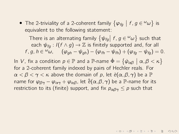
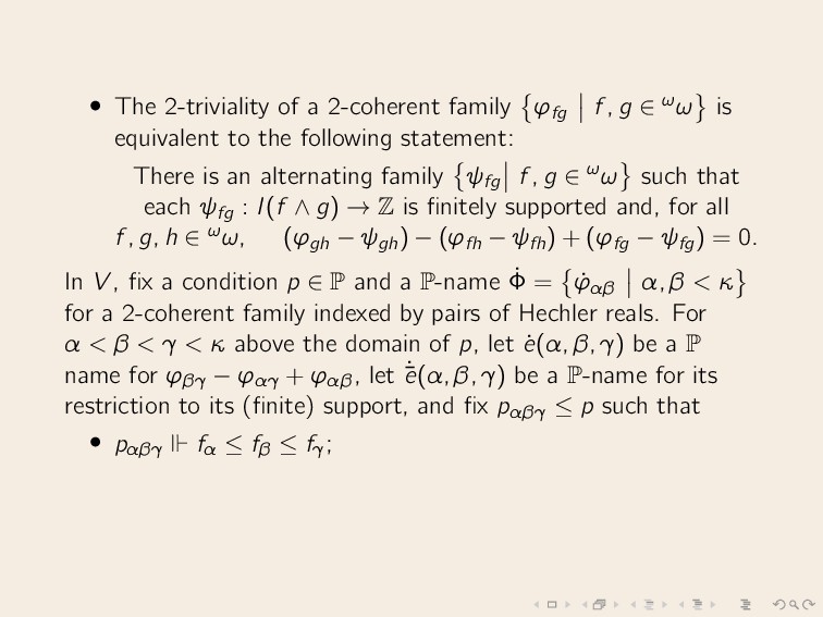
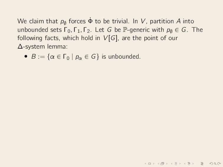
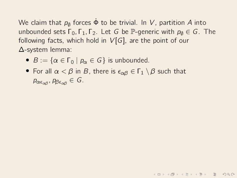
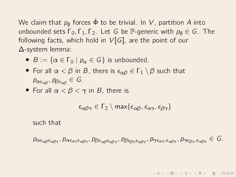
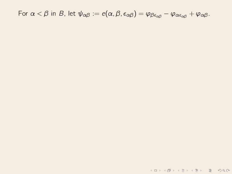
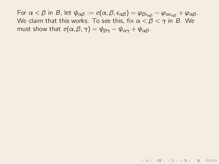
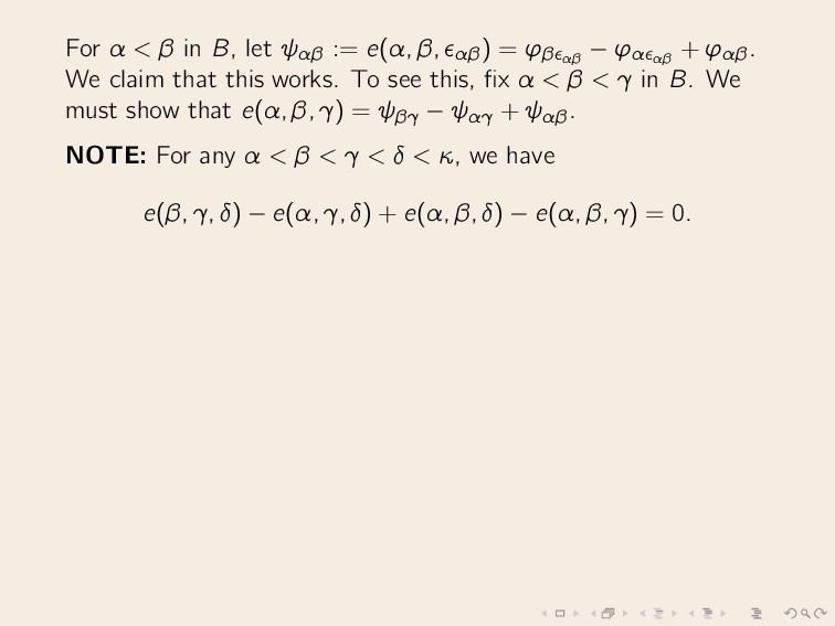
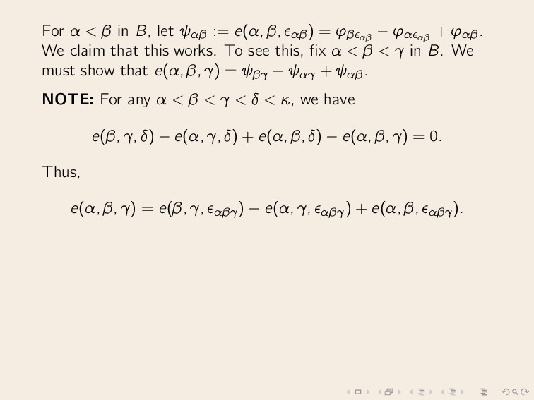
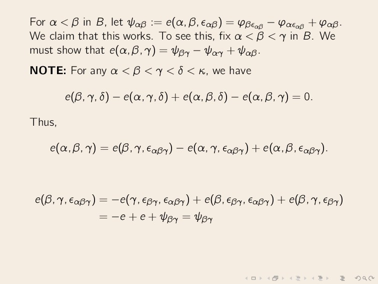
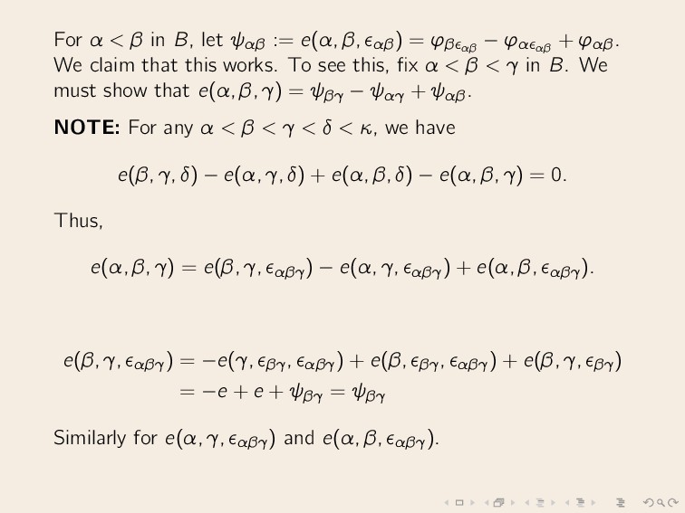
β, αβ) = ϕβ αβ − ϕα αβ + ϕαβ. We claim that this works. To see this, fix α < β < γ in B. We must show that e(α, β, γ) = ψβγ − ψαγ + ψαβ. NOTE: For any α < β < γ < δ < κ, we have e(β, γ, δ) − e(α, γ, δ) + e(α, β, δ) − e(α, β, γ) = 0. Thus, e(α, β, γ) = e(β, γ, αβγ) − e(α, γ, αβγ) + e(α, β, αβγ). e(β, γ, αβγ) = −e(γ, βγ, αβγ) + e(β, βγ, αβγ) + e(β, γ, βγ) = −e + e + ψβγ = ψβγ Similarly for e(α, γ, αβγ) and e(α, β, αβγ). This reduces to e(α, β, γ) = ψβγ − ψαγ + ψαβ, as desired.