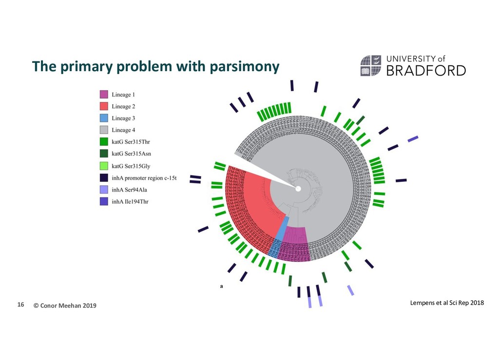
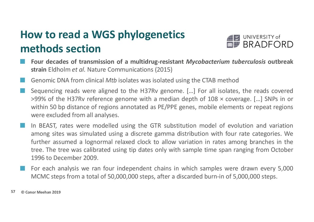
methods section Four decades of transmission of a multidrug-resistant Mycobacterium tuberculosis outbreak strain Eldholm et al. Nature Communications (2015) Genomic DNA from clinical Mtb isolates was isolated using the CTAB method Sequencing reads were aligned to the H37Rv genome. […] For all isolates, the reads covered >99% of the H37Rv reference genome with a median depth of 108 × coverage. […] SNPs in or within 50 bp distance of regions annotated as PE/PPE genes, mobile elements or repeat regions were excluded from all analyses. In BEAST, rates were modelled using the GTR substitution model of evolution and variation among sites was simulated using a discrete gamma distribution with four rate categories. We further assumed a lognormal relaxed clock to allow variation in rates among branches in the tree. The tree was calibrated using tip dates only with sample time span ranging from October 1996 to December 2009. For each analysis we ran four independent chains in which samples were drawn every 5,000 MCMC steps from a total of 50,000,000 steps, after a discarded burn-in of 5,000,000 steps. 2
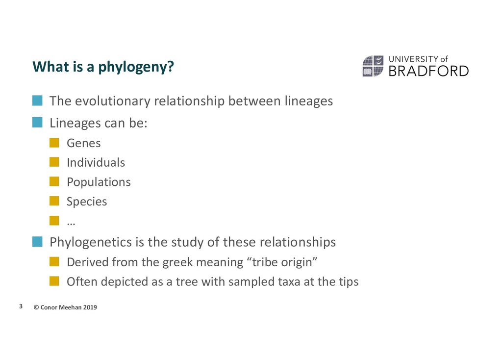
relationship between lineages Lineages can be: Genes Individuals Populations Species … Phylogenetics is the study of these relationships Derived from the greek meaning “tribe origin” Often depicted as a tree with sampled taxa at the tips 3
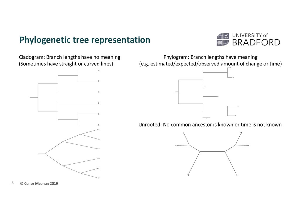
F E A C B D F E A C 0.3 E D B C A F E D B C A F Cladogram: Branch lengths have no meaning (Sometimes have straight or curved lines) Phylogram: Branch lengths have meaning (e.g. estimated/expected/observed amount of change or time) Unrooted: No common ancestor is known or time is not known
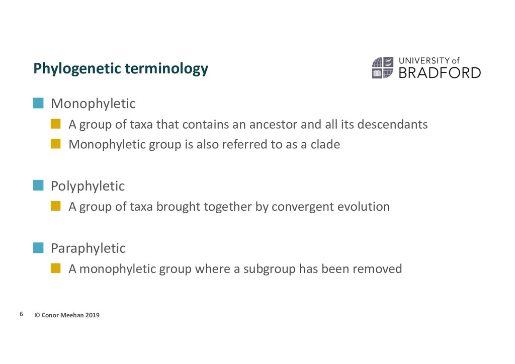
taxa that contains an ancestor and all its descendants Monophyletic group is also referred to as a clade Polyphyletic A group of taxa brought together by convergent evolution Paraphyletic A monophyletic group where a subgroup has been removed 6
al, Sci Rep 2017 Monophyletic M. avium Polyphyletic M. simiae (M. kubicae separate) Paraphyletic M. simiae without M. kubicae (M. avium shares the same ancestor)
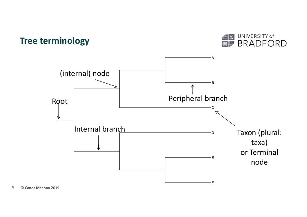
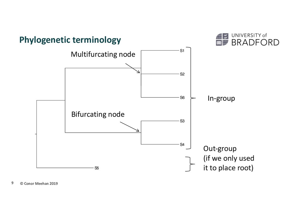
connects only 2 branches Multifurcating (polytomy) A node in a tree which connects more than two branches In-group/out-group In-group is the set of taxa of interest. Assumed to be monophyletic Out-group is a related set of taxa to the in-group, used for rooting 8
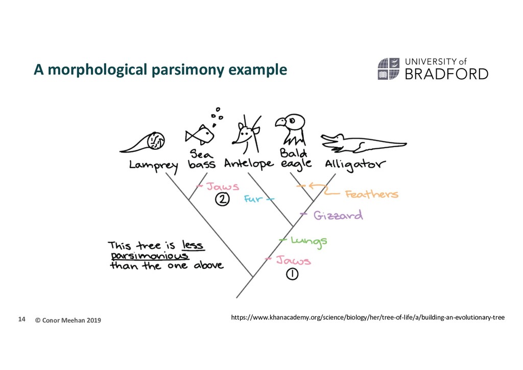
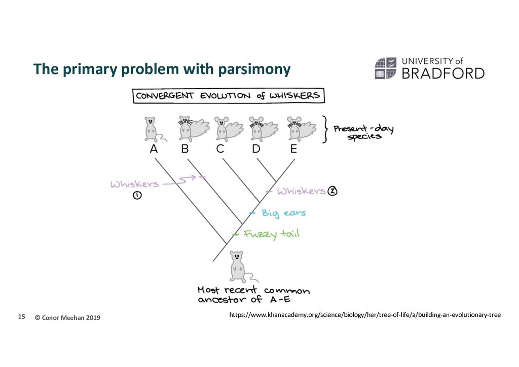
Use an optimality criterion to define how we measure the fit of the data to a solution Tree-search method: how do we decide between possible solutions? Simplest is parsimony Referred to as non-parametric The tree that represents the minimum number of character changes between taxa is the optimal solution 10
Phylogeny is most often undertaken using molecular data Nucleotides/DNA sequence (sometimes RNA sequences) Amino acids/Protein sequence Less sensitive to convergent evolution Parsimony also can be used on molecular data Use G, T, C, A or amino acids as the characters Early tree building used distance based methods Semi-parametric Get a distance between 2 sequences Sequences with shortest distance are most related Most often uses a neighbour joining method 17
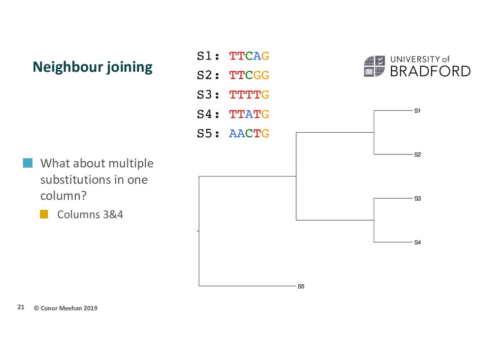
S3 S4 S5 S1 S2 S3 S4 S5 S1: TTCAG S2: TTCGG S3: TTTTG S4: TTATG S5: AACTG Note: count as differences, not as number of characters in common Dissimilarity is differences/total sites
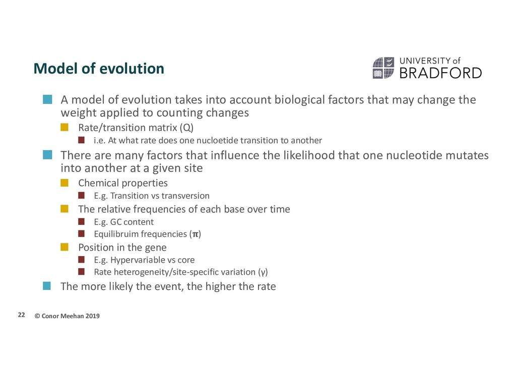
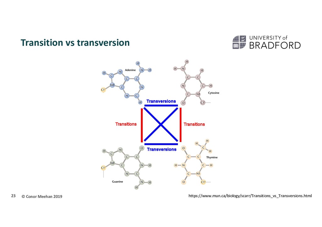
evolution takes into account biological factors that may change the weight applied to counting changes Rate/transition matrix (Q) i.e. At what rate does one nucloetide transition to another There are many factors that influence the likelihood that one nucleotide mutates into another at a given site Chemical properties E.g. Transition vs transversion The relative frequencies of each base over time E.g. GC content Equilibruim frequencies () Position in the gene E.g. Hypervariable vs core Rate heterogeneity/site-specific variation (γ) The more likely the event, the higher the rate 22
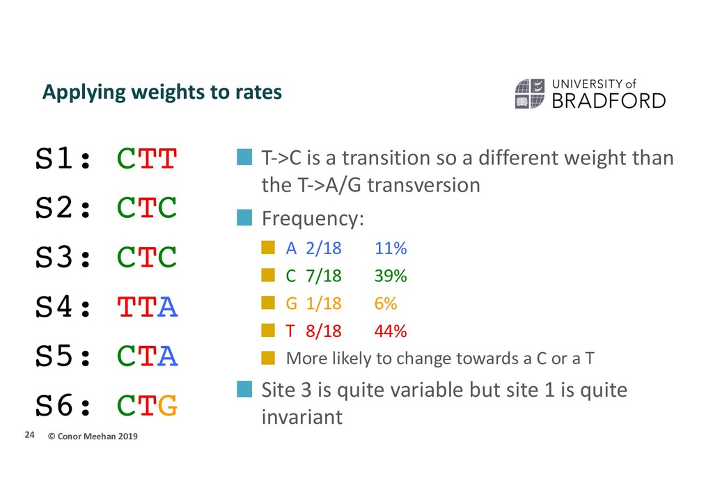
CTT S2: CTC S3: CTC S4: TTA S5: CTA S6: CTG T->C is a transition so a different weight than the T->A/G transversion Frequency: A 2/18 11% C 7/18 39% G 1/18 6% T 8/18 44% More likely to change towards a C or a T Site 3 is quite variable but site 1 is quite invariant
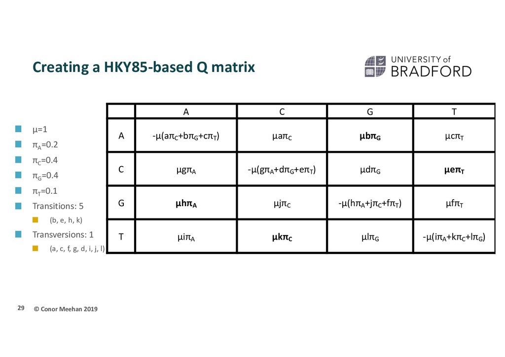
instantaneous substitution rate If measuring as substitutions μ=1 If measuring as time, this is the mutation rate a,b,c,...l = rate parameter for each possible transformation of one base to another πA = frequency of bases A, C, G, T Transitions are in bold 25 A C G T A -μ(aπC +bπG +cπT ) μaπC μbπG μcπT C μgπA -μ(gπA +dπG +eπT ) μdπG μeπT G μhπA μjπC -μ(hπA +jπC +fπT ) μfπT T μiπA μkπC μlπG -μ(iπA +kπC +lπG )
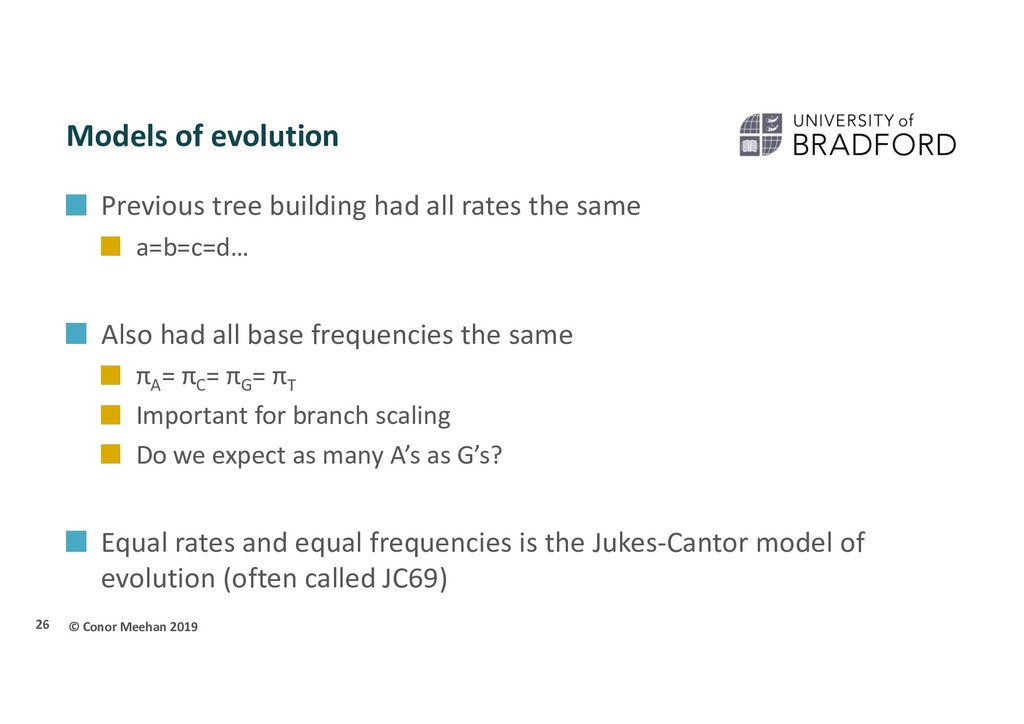
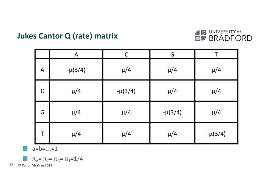
had all rates the same a=b=c=d… Also had all base frequencies the same πA = πC = πG = πT Important for branch scaling Do we expect as many A’s as G’s? Equal rates and equal frequencies is the Jukes-Cantor model of evolution (often called JC69) 26
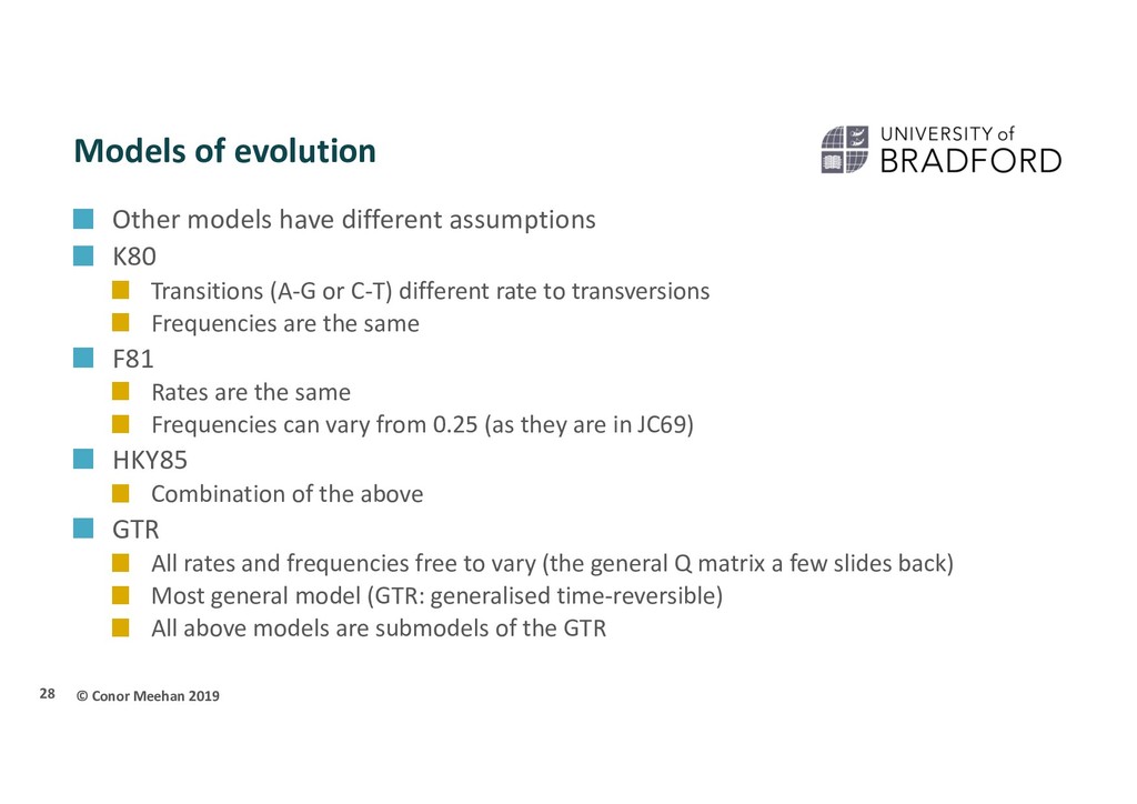
different assumptions K80 Transitions (A-G or C-T) different rate to transversions Frequencies are the same F81 Rates are the same Frequencies can vary from 0.25 (as they are in JC69) HKY85 Combination of the above GTR All rates and frequencies free to vary (the general Q matrix a few slides back) Most general model (GTR: generalised time-reversible) All above models are submodels of the GTR 28
πA =0.2 πC =0.4 πG =0.4 πT =0.1 Transitions: 5 (b, e, h, k) Transversions: 1 (a, c, f, g, d, i, j, l) 30 A C G T A -1(1*0.4+5*0.4+1*0.1) 1*1*0.4 1*5*0.4 1*1*0.1 C 1*1*0.2 -1(1*0.2+1*0.4+5*0.1) 1*1*0.4 1*5*0.1 G 1*5*0.2 1*1*0.4 -1(5*0.2+1*0.4+1*0.1) 1*1*0.1 T 1*1*0.2 1*5*0.4 1*1*0.4 -1(1*0.2+5*0.4+1*0.4)
πA =0.2 πC =0.4 πG =0.4 πT =0.1 Transitions: 5 (b, e, h, k) Transversions: 1 (a, c, f, g, d, i, j, l) 31 A C G T A -2.5 0.4 2 0.1 C 0.2 -1.1 0.4 0.5 G 1 0.4 -1.5 0.1 T 0.2 2 0.4 -2.6
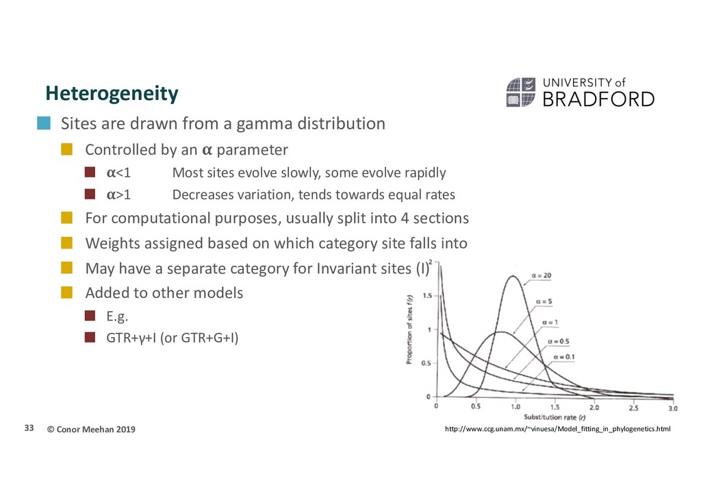
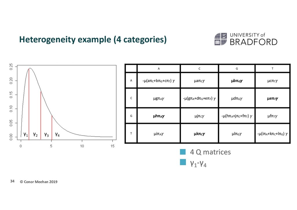
nucleotides may differ between sites Thus, we may wish to give more/less weight to differences in an area of high/low variation Hypervariable vs structural regions In models of evolution, this is often represented as a gamma (γ) parameter 32
gamma distribution Controlled by an parameter <1 Most sites evolve slowly, some evolve rapidly >1 Decreases variation, tends towards equal rates For computational purposes, usually split into 4 sections Weights assigned based on which category site falls into May have a separate category for Invariant sites (I) Added to other models E.g. GTR+γ+I (or GTR+G+I) 33 http://www.ccg.unam.mx/~vinuesa/Model_fitting_in_phylogenetics.html
C G T A -μ(aπC+bπG+cπT) μaπC μbπG μcπT C μgπA -μ(gπA+dπG+eπT) μdπG μeπT G μhπA μjπC -μ(hπA+jπC+fπT) μfπT T μiπA μkπC μlπG -μ(iπA+kπC+lπG) γ1 γ2 γ3 γ4 4 Q matrices γ1 -γ4
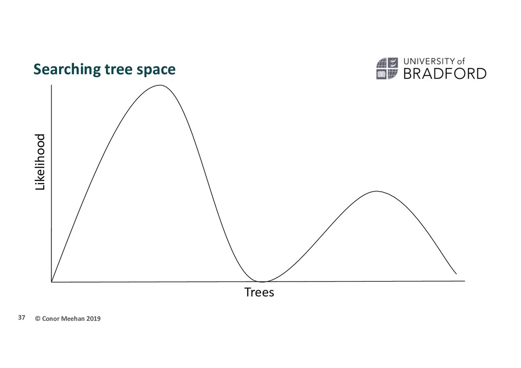
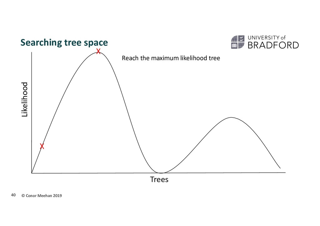
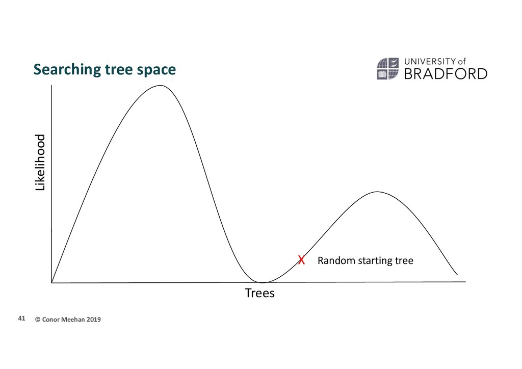
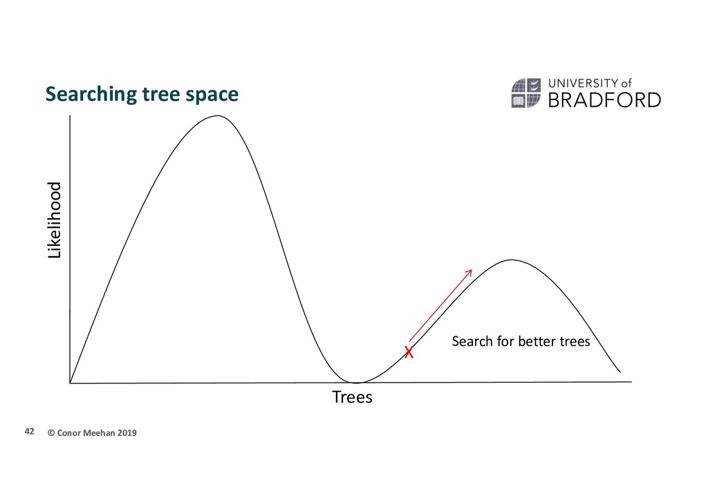
seen methods take 2 sequences and calculate a distance and continue in a pairwise manner through the whole set of sequences Parametric methods take a column in an alignment and calculate the optimality criterion per site Sites are independent An explicit model of evolution is required Can incorporate rate heterogeneity There are two main parametric methods of phylogenetic inference: Maximum likelihood Bayesian analysis Both methods search tree space to find the best tree 35
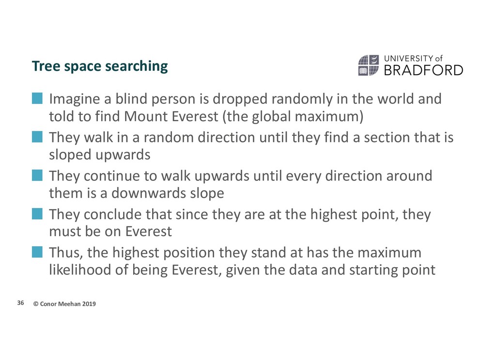
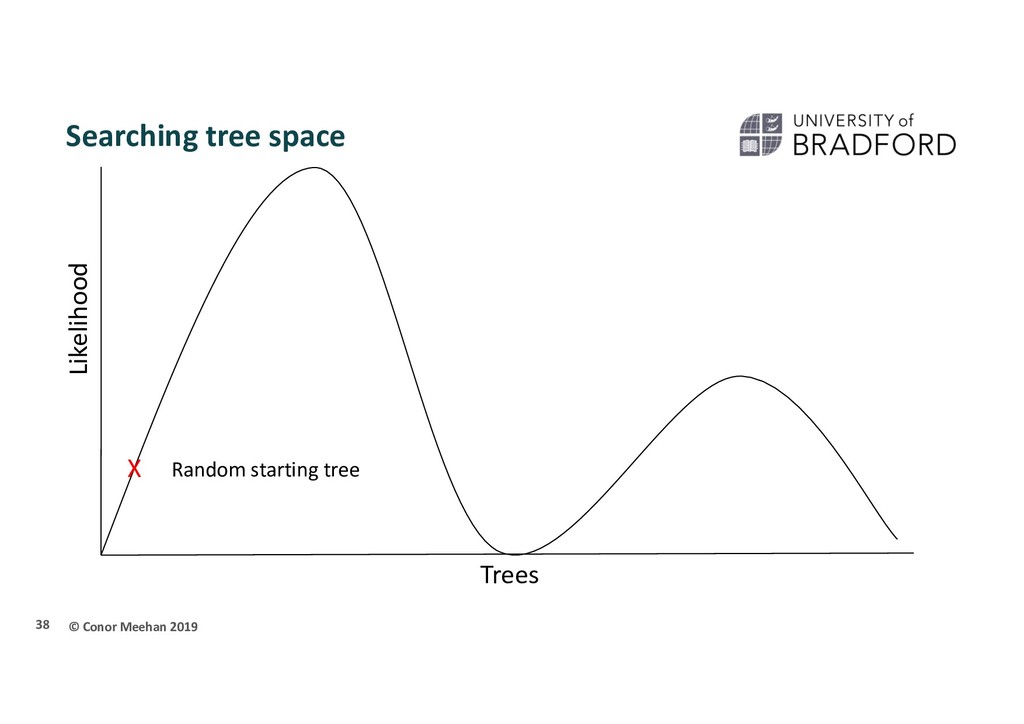
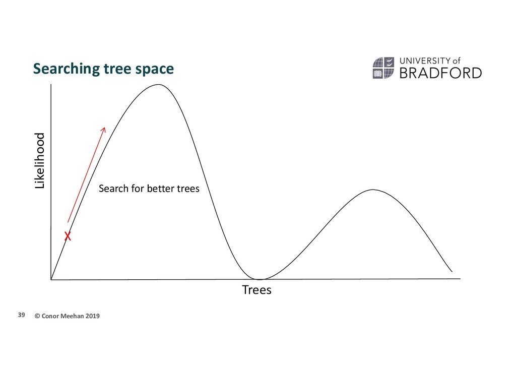
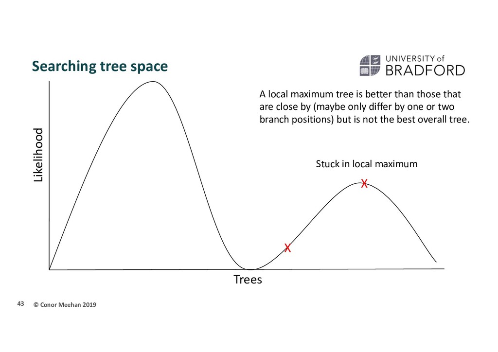
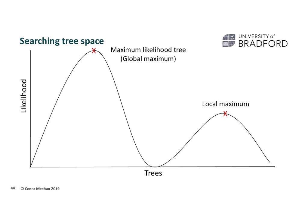
person is dropped randomly in the world and told to find Mount Everest (the global maximum) They walk in a random direction until they find a section that is sloped upwards They continue to walk upwards until every direction around them is a downwards slope They conclude that since they are at the highest point, they must be on Everest Thus, the highest position they stand at has the maximum likelihood of being Everest, given the data and starting point 36
X Stuck in local maximum X A local maximum tree is better than those that are close by (maybe only differ by one or two branch positions) but is not the best overall tree.
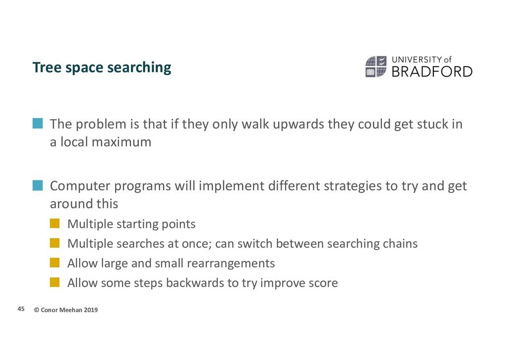
that if they only walk upwards they could get stuck in a local maximum Computer programs will implement different strategies to try and get around this Multiple starting points Multiple searches at once; can switch between searching chains Allow large and small rearrangements Allow some steps backwards to try improve score 45
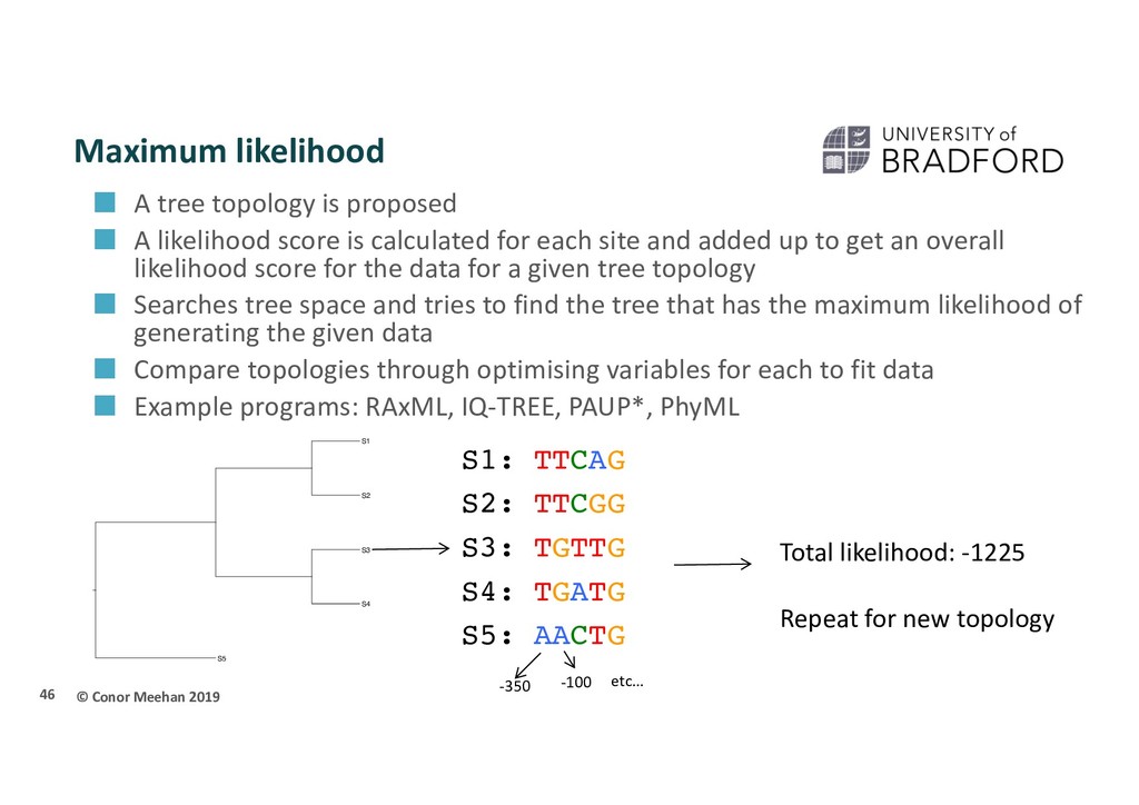
proposed A likelihood score is calculated for each site and added up to get an overall likelihood score for the data for a given tree topology Searches tree space and tries to find the tree that has the maximum likelihood of generating the given data Compare topologies through optimising variables for each to fit data Example programs: RAxML, IQ-TREE, PAUP*, PhyML 46 S3 S5 S2 S4 S1 S1: TTCAG S2: TTCGG S3: TGTTG S4: TGATG S5: AACTG -350 -100 etc… Total likelihood: -1225 Repeat for new topology
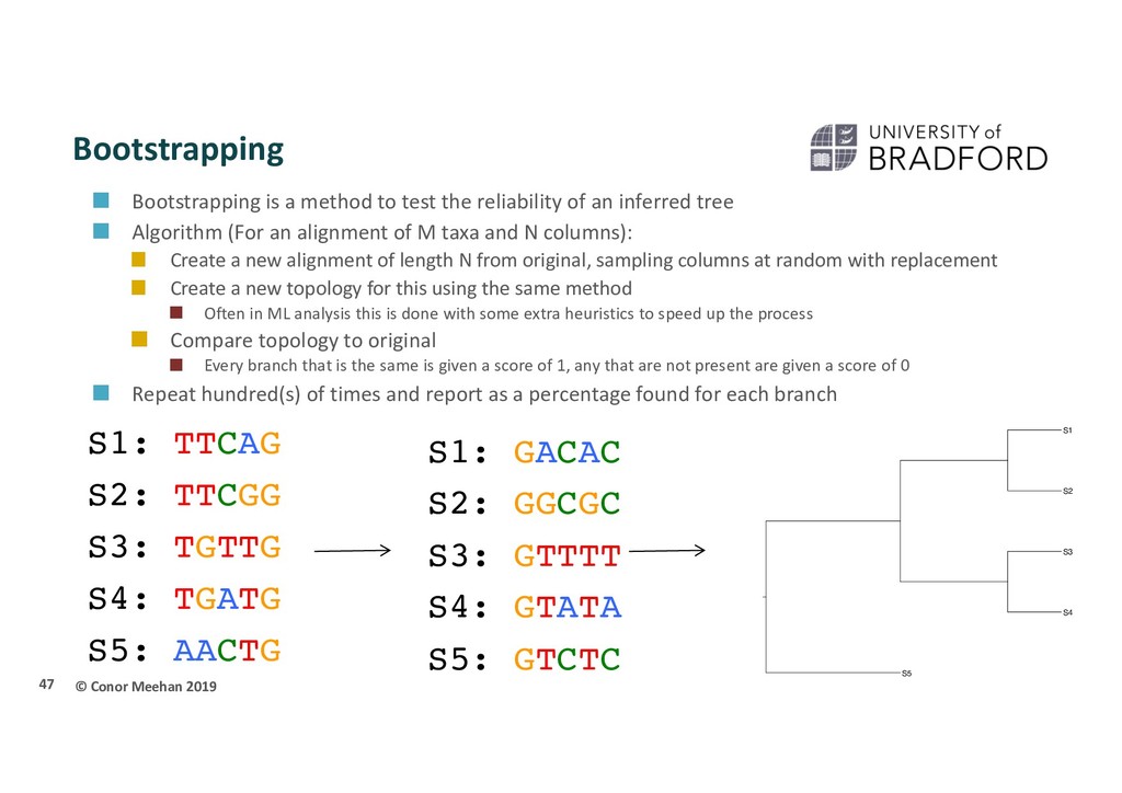
test the reliability of an inferred tree Algorithm (For an alignment of M taxa and N columns): Create a new alignment of length N from original, sampling columns at random with replacement Create a new topology for this using the same method Often in ML analysis this is done with some extra heuristics to speed up the process Compare topology to original Every branch that is the same is given a score of 1, any that are not present are given a score of 0 Repeat hundred(s) of times and report as a percentage found for each branch 47 S3 S5 S2 S4 S1 S1: GACAC S2: GGCGC S3: GTTTT S4: GTATA S5: GTCTC S1: TTCAG S2: TTCGG S3: TGTTG S4: TGATG S5: AACTG
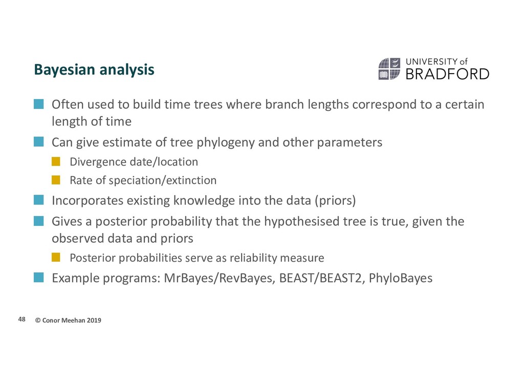
time trees where branch lengths correspond to a certain length of time Can give estimate of tree phylogeny and other parameters Divergence date/location Rate of speciation/extinction Incorporates existing knowledge into the data (priors) Gives a posterior probability that the hypothesised tree is true, given the observed data and priors Posterior probabilities serve as reliability measure Example programs: MrBayes/RevBayes, BEAST/BEAST2, PhyloBayes 48
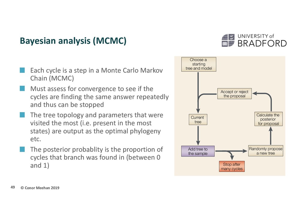
a step in a Monte Carlo Markov Chain (MCMC) Must assess for convergence to see if the cycles are finding the same answer repeatedly and thus can be stopped The tree topology and parameters that were visited the most (i.e. present in the most states) are output as the optimal phylogeny etc. The posterior probablity is the proportion of cycles that branch was found in (between 0 and 1) 49 Consider using a phylogenetic analysis to determine whether an unknown virus belongs to ‘group A’ or ‘group B’.A tree with representatives of both candidate groups and the unknown sample is constructed, and used to overcome an inappropriate analysis of the data. It might be said that high bootstrap proportions are a necessary, but not sufficient, condition for having high confidence in a group. are stricter.From an initial tree,a new tree is proposed.The moves that change the tree must involve a random choice that satisfies several conditions43,44.The MCMC algorithm also specifies the rules for when to accept or reject a tree. Note that MCMC yields a much larger sample of trees in the same computational time, because it produces one tree for every proposal cycle versus one tree per tree search (which assesses numerous alternative trees) in the traditional approach. However, the sample of trees produced by MCMC is highly auto-correlated.As a result, millions of cycles through MCMC are usually required, whereas many fewer (of the order of 1,000) bootstrap replicates are sufficient for most problems. Tree search Aligned data matrix and model Generate pseudo-replicate data matrix Bootstrap the data Current tree Score the new tree Accept or reject new tree Propose a new tree Stop after many cycles Add final tree to the sample a Choose a starting tree and model Randomly propose a new tree Stop after many cycles Add tree to the sample Current tree Accept or reject the proposal Calculate the posterior for proposal b
knowledge that applies to the data, we can incorporate this into the model Sampling dates Model of evolution Fossil dates For instance we may have a dataset of an outbreak that started in 2009 and we can limit the estimates of time on a tree to be that year at maximum These help guide the process through tree searching space Wrong priors give wrong estimates Can/Must also incorporate evolutionary/population processes into the model Time trees requires a molecular clock model Population size estimates require a population model Can also test which is appropriate within the framework 50
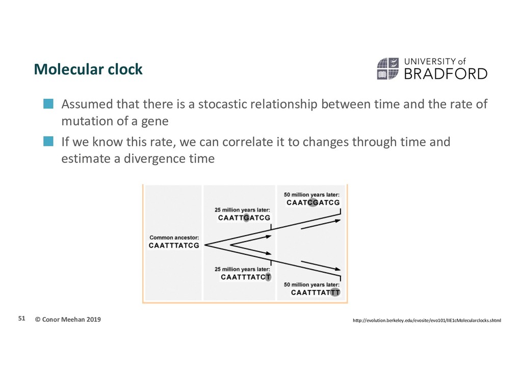
a stocastic relationship between time and the rate of mutation of a gene If we know this rate, we can correlate it to changes through time and estimate a divergence time 51 http://evolution.berkeley.edu/evosite/evo101/IIE1cMolecularclocks.shtml
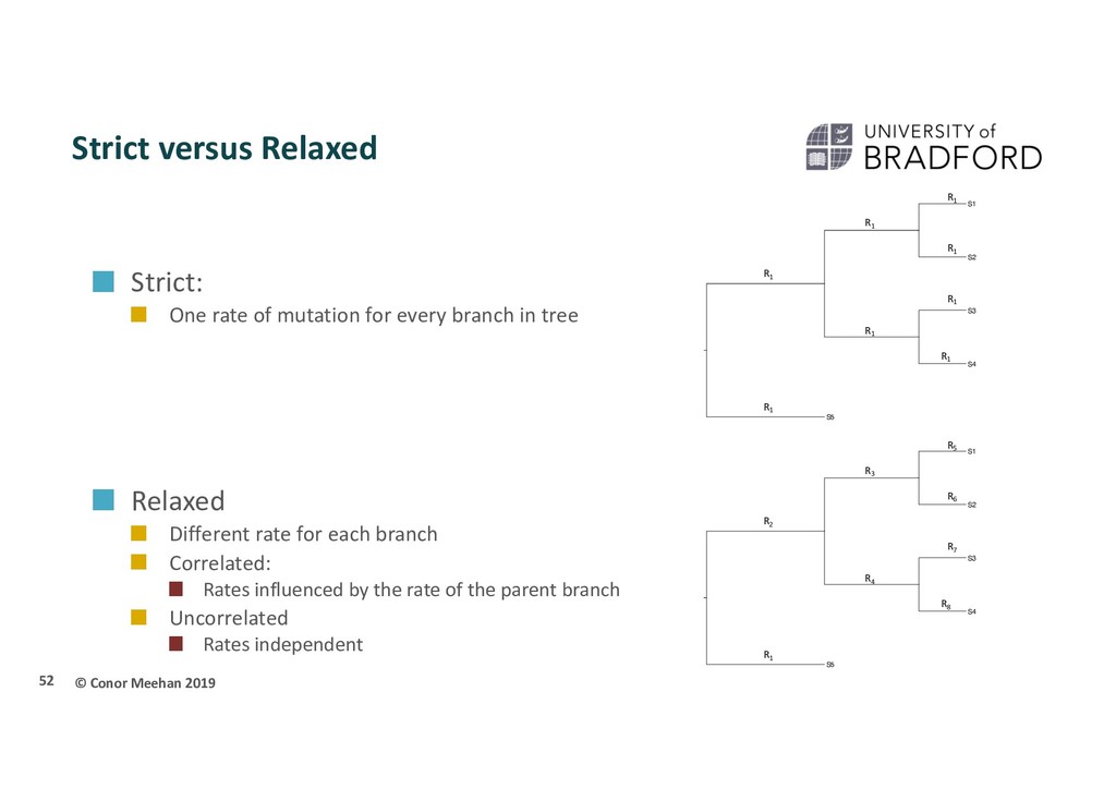
of mutation for every branch in tree Relaxed Different rate for each branch Correlated: Rates influenced by the rate of the parent branch Uncorrelated Rates independent 52 S3 S5 S2 S4 S1 R1 R1 R1 R1 R1 R1 R1 R1 S3 S5 S2 S4 S1 R7 R6 R5 R8 R4 R1 R2 R3
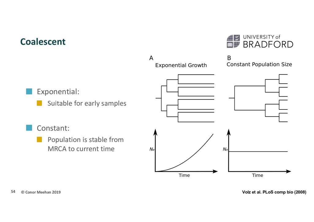
When two alleles/individuals come together to form an ancestor (i.e. two branches meet) this is called a coalescent event 53 Sainani Biomedical computation review (2009)
ascertainment bias problem Only selected the variable sites Invariant sites affect branch lengths Nucleotide frequencies Change at every position vs change at a few Small branch lengths may change topologies Can correct for this with ascertainment bias correction Tell method number of invariant sites Total count Per nucleotide 55
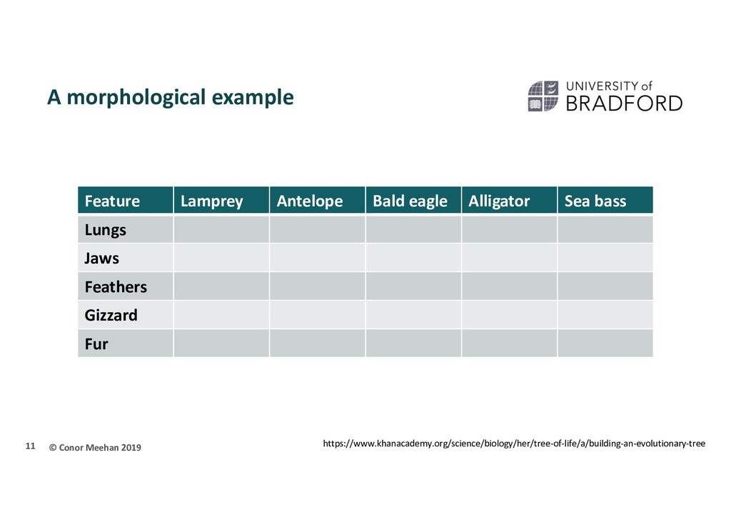
done on morphological or molecular data Molecular less likely to be affected by convergent evolution Many methods for building trees exist, each with its own criteria for the best fit for the data Parsimony Distance Maximum Likelihood/Bayesian Most methods require a model of evolution to give information on how the sequences evolved Complex algorithms such as ML or Bayesian require efficient searching of the tree space Ascertainment bias can skew the results if only SNPs are used. 56
methods section Four decades of transmission of a multidrug-resistant Mycobacterium tuberculosis outbreak strain Eldholm et al. Nature Communications (2015) Genomic DNA from clinical Mtb isolates was isolated using the CTAB method Sequencing reads were aligned to the H37Rv genome. […] For all isolates, the reads covered >99% of the H37Rv reference genome with a median depth of 108 × coverage. […] SNPs in or within 50 bp distance of regions annotated as PE/PPE genes, mobile elements or repeat regions were excluded from all analyses. In BEAST, rates were modelled using the GTR substitution model of evolution and variation among sites was simulated using a discrete gamma distribution with four rate categories. We further assumed a lognormal relaxed clock to allow variation in rates among branches in the tree. The tree was calibrated using tip dates only with sample time span ranging from October 1996 to December 2009. For each analysis we ran four independent chains in which samples were drawn every 5,000 MCMC steps from a total of 50,000,000 steps, after a discarded burn-in of 5,000,000 steps. 57
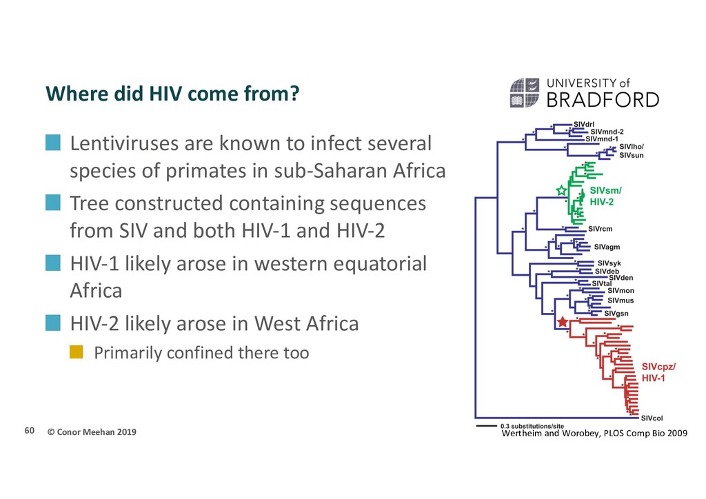
are known to infect several species of primates in sub-Saharan Africa Tree constructed containing sequences from SIV and both HIV-1 and HIV-2 HIV-1 likely arose in western equatorial Africa HIV-2 likely arose in West Africa Primarily confined there too 60 Wertheim and Worobey, PLOS Comp Bio 2009
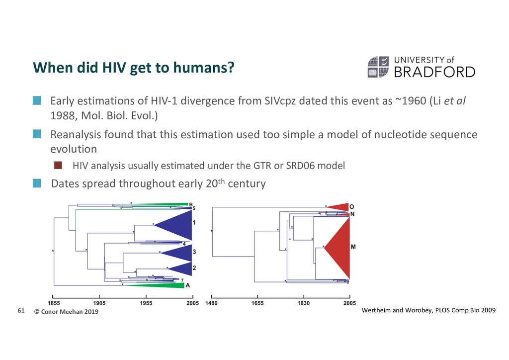
61 Wertheim and Worobey, PLOS Comp Bio 2009 Early estimations of HIV-1 divergence from SIVcpz dated this event as ~1960 (Li et al 1988, Mol. Biol. Evol.) Reanalysis found that this estimation used too simple a model of nucleotide sequence evolution HIV analysis usually estimated under the GTR or SRD06 model Dates spread throughout early 20th century
62 An early hypothesis, outlined in ‘The River’ by Edward Hooper (1999) suggested a a contaminated oral polio vaccine (OPV) used in the 1950’s The other leading hypothesis is that blood-to-blood transmission occurred from butchered primate meat to hunters Molecular evidence was gathered by Sharp et al (2001, Phil. Trans. R. Soc. Lond. B) to review these claims OPV trial chimpanzees were not the same as those suggested to be resevoir for SIV The origins were dated as ~1931, not 1950’ Although the bush meat hypothesis cannot be directly proven, phylogenetic and molecular analysis lend strong support against the OPV hypothesis
transmission Intentional or negligent transmission of HIV can result in charges of assault, manslaughter or murder in several countries Two things often must be proven for this: The defendant was reckless The defendant infected the complainant In the UK it was required that scientific evidence must be used to prove infection, even if a plea of ‘guilty’ was entered Phylogenetics is often used in this step Phylogenetics is often required to prove recklessness too Time of infection must be after the defendant became aware of their status and before the complainant became aware of the defendant’s status 64
transmission First used in 1990 in a case of a dentist infecting several patients though this case never went to court First used in a criminal case in Sweden in 1992, though directionality was not determined In 2002 phylogenetic analysis was used to uphold a conviction during appeal by a gastroenterologist in the 2nd degree murder charge of his girlfriend after it had been found to meet standards of evidence admissibility 65
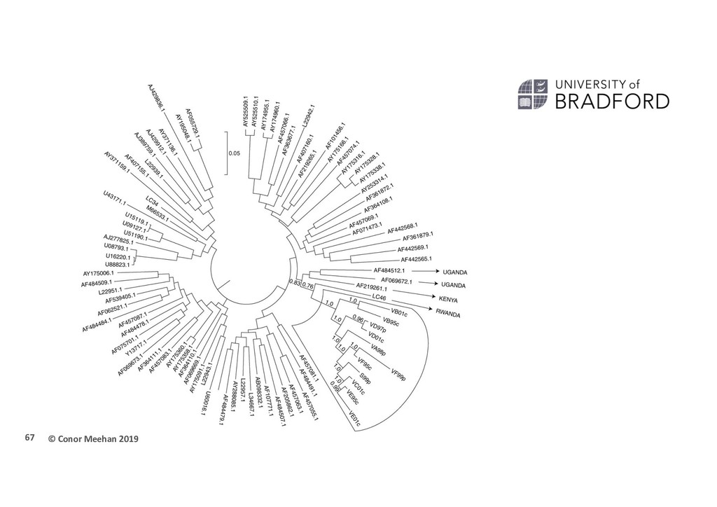
transmission Lemey et al. “Molecular testing of multiple HIV-1 transmissions in a criminal case”, AIDS 19(15), 2005 One suspect and six victims 2 samples from each person, anonymously labelled and sequenced for pol and env fragments 30 controls taken from local hospital fitting as closely to the age, risk and geographical parameters as the suspect/victims and from around the same time of alleged transmission as possible Phylogenetic trees built under ML using 3 methods and also using Bayesian inference Sites known to infer drug resistance were excluded to prevent clustering based on drug regimes 66
and victim samples, monophyletic to the exclusion of controls No inference was made about directionality (usually indicated by paraphyletic relationship of source sequences around recipient sequences) Cannot rule out case of both suspect and victim infected by a 3rd person or suspect infecting a person who infected victims Local control selection is critical 68
headache, coughing, nasal discharge 250-500k deaths a year Caused by Influenza virus Three types (A-C) A causes all pandemics Serotypes based on hemagglutinin (H/HA) and neuraminidase (N/NA) E.g. Influenza A H1N1 (”Spanish flu” or ‘Swine flu”) 70
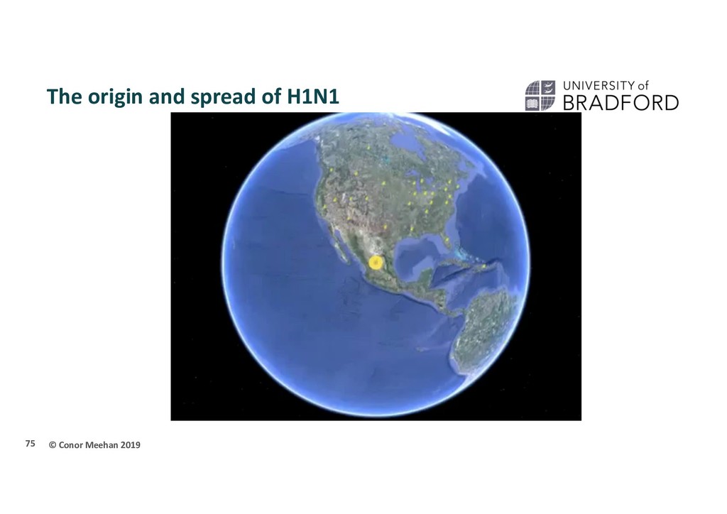
(swine flu) influenza strain was first identified in April 2009 Within a few months it reached pandemic proportions Phylogeographic analysis Where did the outbreak start? How and when did it spread? 71
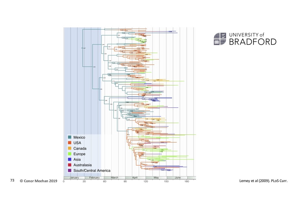
al (2009), “Reconstructing the initial global spread of a human influenza pandemic” PLOS currents 242 sequences HA and NA gene sequences 40 locations worldwide 30th March to 12th July 2009 Bayesian framework HKY + gamma model Relaxed molecular clock BSSVS model of spatial diffusion Bayesian stochastic search variable selection 7 discrete locations as priors Allow MCMC to assign location probabilities to internal nodes 72
Phylogenetic reconstruction indicates Mexico as the likely origin of the virus Several USA strains were seeded early in the outbreak Most European lineages came from USA strains, not Mexico 74
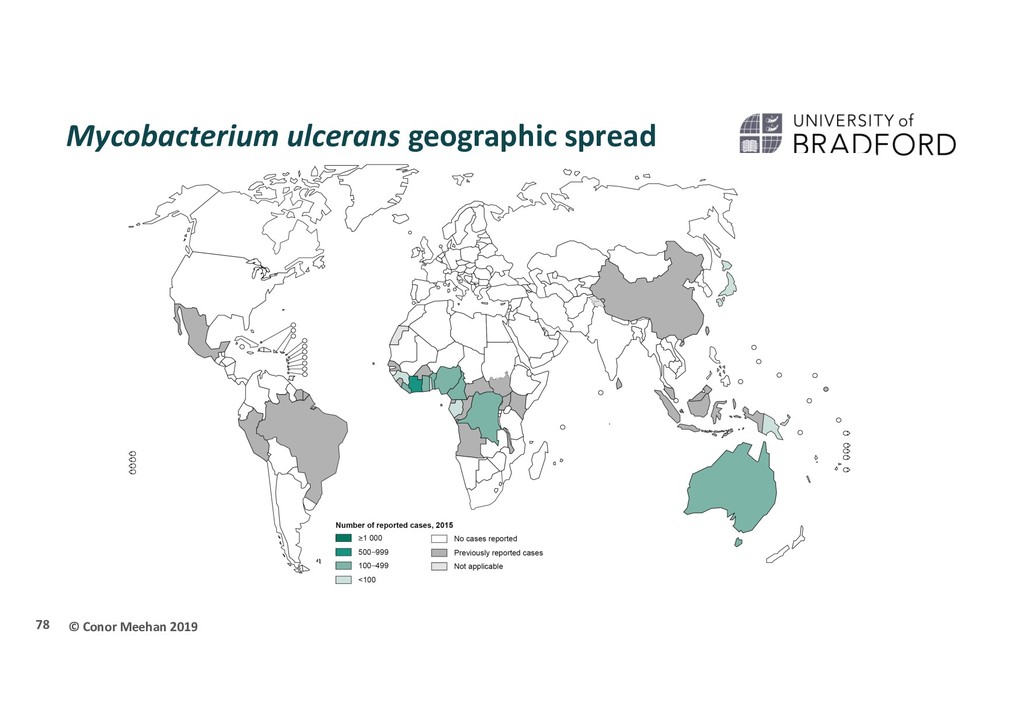
Ulcer (BU) ~ 6000 cases a year (declining) Causes skin ulceration and sometimes bone involvement M. ulcerans produces a toxin, mycolactone, which damages tissue WARNING: photos! 77
directly human to human Proximity to slow flowing/stagnant water Prevailing hypothesis: Environmental species that infects after microtrauma Do humans play a role in the spread of MU? 79
population structure and evolutionary history of MU in Africa? 165 isolates 1964-2012 Most endemic African countries Papua New Guinea outgroup Illumina reads assembled with Snippy pipeline SNP alignment Recombination free 9,193 SNPs 80
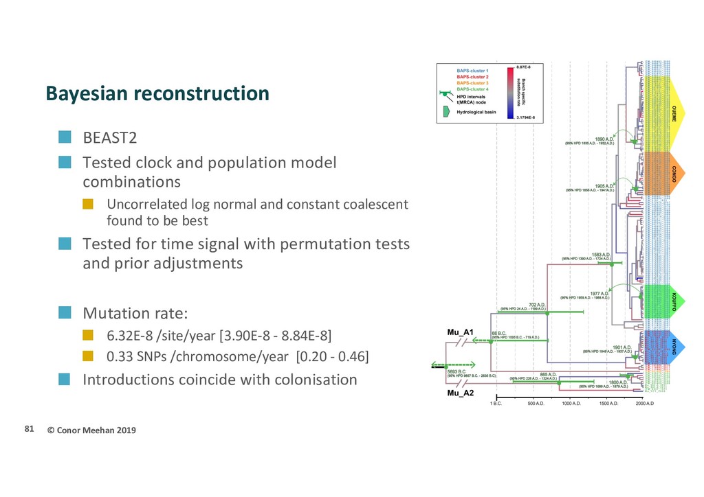
population model combinations Uncorrelated log normal and constant coalescent found to be best Tested for time signal with permutation tests and prior adjustments Mutation rate: 6.32E-8 /site/year [3.90E-8 - 8.84E-8] 0.33 SNPs /chromosome/year [0.20 - 0.46] Introductions coincide with colonisation 81
Africa Slow evolving bacterium One of the slowest rates recorded Clonal expansion with no recombination Multiple introductions Each major lineage introduced separately Likely began in South-East Asia (still be confirmed) Exact place of first introduction into Africa not known (perhaps central) Potentially spread by humans Infected Africans moved to new area during ’Scramble for Africa’ Shed into water which then infects new hosts Will treatment of humans decline the environmental population too? Population modelling suggests yes 82
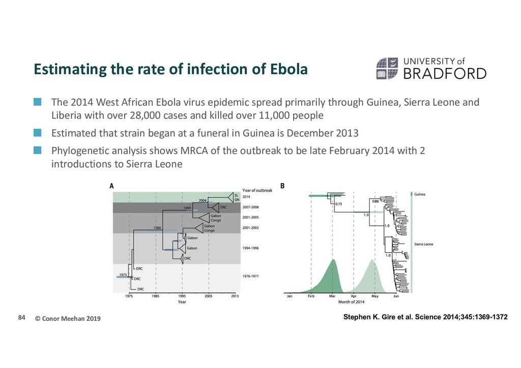
Ebola The 2014 West African Ebola virus epidemic spread primarily through Guinea, Sierra Leone and Liberia with over 28,000 cases and killed over 11,000 people Estimated that strain began at a funeral in Guinea is December 2013 Phylogenetic analysis shows MRCA of the outbreak to be late February 2014 with 2 introductions to Sierra Leone 84 Stephen K. Gire et al. Science 2014;345:1369-1372
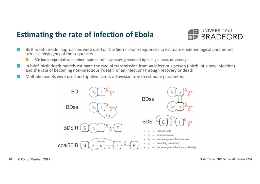
Ebola Birth-death model approaches were used on the Sierra Leone sequences to estimate epidemiological parameters across a phylogeny of the sequences R0: basic reprodutive number; number of new cases generated by a single case, on average In brief, birth death models estimate the rate of transmission from an infectious person (‘birth’ of a new infection) and the rate of becoming non-infectious (‘death’ of an infection) through recovery or death Multiple models were used and applied across a Bayesian tree to estimate parameters 85 Stadler T et al. PLOS Currents Outbreaks. 2014
Ebola R0 : ~2.18 (range 1.24 - 3.55) Incubation time: ~4.92 days Infectious period: ~2.58 days Thus on average 2 people will be infected by every infected individual This is low when compared to some other common pathogens. E.g.: Influenza: 2-3 HIV: 2-5 Measles: 12-18 86
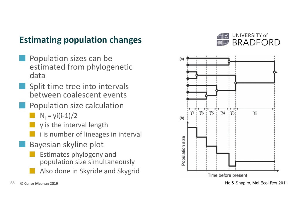
be estimated from phylogenetic data Split time tree into intervals between coalescent events Population size calculation Ni = γi(i-1)/2 γ is the interval length i is number of lineages in interval Bayesian skyline plot Estimates phylogeny and population size simultaneously Also done in Skyride and Skygrid 88 Ho & Shapiro, Mol Ecol Res 2011
and cirrhosis Caused by the Hepatitis C virus (HCV) 130-200M infected worldwide ~700,000 deaths a year Blood to blood contact Unsterilized equipment 89
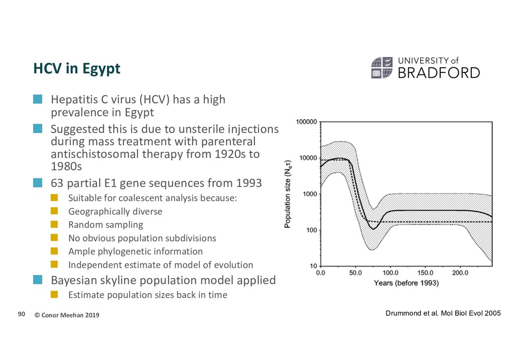
(HCV) has a high prevalence in Egypt Suggested this is due to unsterile injections during mass treatment with parenteral antischistosomal therapy from 1920s to 1980s 63 partial E1 gene sequences from 1993 Suitable for coalescent analysis because: Geographically diverse Random sampling No obvious population subdivisions Ample phylogenetic information Independent estimate of model of evolution Bayesian skyline population model applied Estimate population sizes back in time 90 Drummond et al. Mol Biol Evol 2005
ruminants High fever Blisters Caused by FMD virus (FMDV) RNA virus 7 serotypes High mutation rate Highly contagious Spread by aerosols and contaminated equipment etc. O CATHAY FMDV Asian topotype Primarily restricted to a given region How is it maintained and dispersed? 92
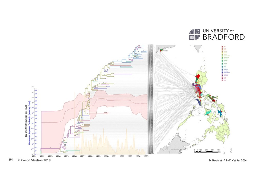
et al (2014) “Phylodynamic reconstruction of O CATHAY topotype foot-and-mouth disease virus epidemics in the Philippines” BMC Vet Res 322 VP1 FMDV sequences 112 Phillippines 1994-2005 22 provinces 210 worldwide Bayesian analysis HKY + gamma Relaxed uncorrelated clock Bayesian skyline BSSVS 93
1.25 x 10⁻² nt/site/year Introduction and spread 30th March 1994 1st wave: Rizal province 2nd wave: Bulacan province 3rd wave: Manila province 3 phase population dynamics Increase until 1997 Intervention in 1996 resulted in sharp decline Reintroduction into Pinay in 1999 cause increase Plateau reached in until end of sampling 95
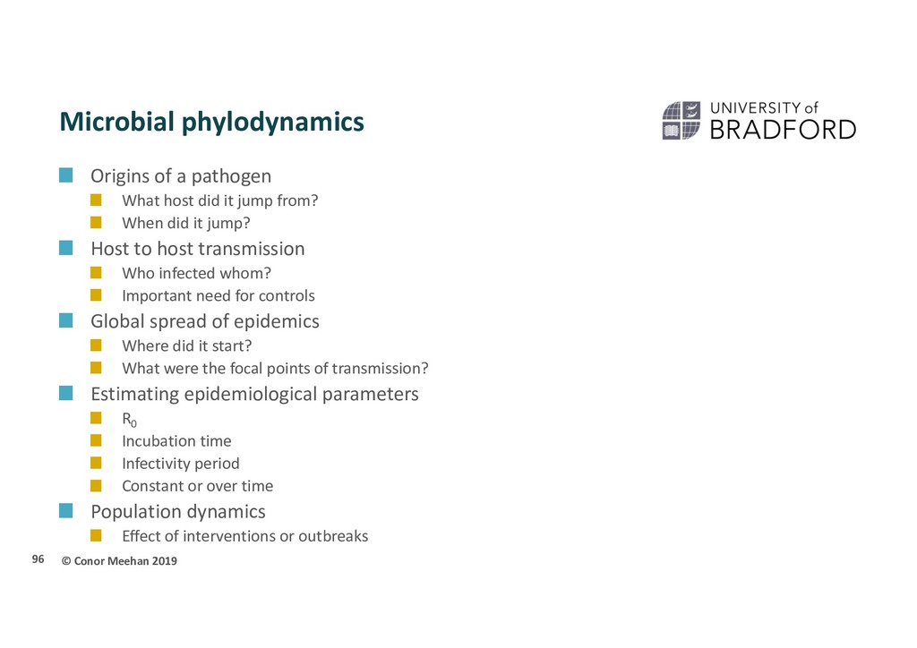
What host did it jump from? When did it jump? Host to host transmission Who infected whom? Important need for controls Global spread of epidemics Where did it start? What were the focal points of transmission? Estimating epidemiological parameters R0 Incubation time Infectivity period Constant or over time Population dynamics Effect of interventions or outbreaks 96