Hackers Statistics

Stats for hackers

Transcript

1. Jake VanderPlas PyCon 2016
2. < About Me > - Astronomer by training - Statistician by accident - Active in Python science & open source - Data Scientist at UW eScience Institute - @jakevdp on Twitter & Github
4. Hacker (n.) 1. A person who is trying to steal your grandma’s bank password.
5. Hacker (n.) 1. A person who is trying to steal your grandma’s bank password. 2. A person whose natural approach to problem-solving involves writing code.
6. Statistics is Hard.
7. Statistics is Hard. Using programming skills, it can be easy.
8. My thesis today: If you can write a for-loop, you can do statistics
9. Statistics is fundamentally about Asking the Right Question.
10. – Dr. Seuss (attr)
11. Warm-up
12. You toss a coin 30 times and see 22 heads. Is it a fair coin? Warm-up: Coin Toss
13. A fair coin should show 15 heads in 30 tosses. This coin is biased. Even a fair coin could show 22 heads in 30 tosses. It might be just chance.
14. Classic Method: Assume the Skeptic is correct: test the Null Hypothesis. What is the probability of a fair coin showing 22 heads simply by chance?
15. Classic Method: Start computing probabilities . . .
16. Classic Method:
17. Classic Method: Number of arrangements (binomial coefficient) Probability of N H heads Probability of N T tails
18. Classic Method:
19. Classic Method:
20. Classic Method: 0.8 %
21. Classic Method: 0.8 % Probability of 0.8% (i.e. p = 0.008) of observations given a fair coin. → reject fair coin hypothesis at p < 0.05
22. Could there be an easier way?
23. Easier Method: Just simulate it! M = 0 for i in range(10000): trials = randint(2, size=30) if (trials.sum() >= 22): M += 1 p = M / 10000 # 0.008149 → reject fair coin at p = 0.008
24. In general . . . Computing the Sampling Distribution is Hard.
25. In general . . . Computing the Sampling Distribution is Hard. Simulating the Sampling Distribution is Easy.
26. Four Recipes for Hacking Statistics: 1. Direct Simulation 2. Shuffling 3. Bootstrapping 4. Cross Validation
27. Now, the Star-Belly Sneetches had bellies with stars. The Plain-Belly Sneetches had none upon thars . . . Sneeches: Stars and Intelligence *inspired by John Rauser’s Statistics Without All The Agonizing Pain
28. ★ ❌ 84 72 81 69 57 46 74 61 63 76 56 87 99 91 69 65 66 44 62 69 ★ mean: 73.5 ❌ mean: 66.9 difference: 6.6 Sneeches: Stars and Intelligence Test Scores
29. ★ mean: 73.5 ❌ mean: 66.9 difference: 6.6 Is this difference of 6.6 statistically significant?
30. Classic Method (Welch’s t-test)
31. Classic Method (Welch’s t-test)
32. Classic Method (Student’s t distribution)
33. Classic Method (Student’s t distribution) Degree of Freedom: “The number of independent ways by which a dynamic system can move, without violating any constraint imposed on it.” -Wikipedia
34. Degree of Freedom: “The number of independent ways by which a dynamic system can move, without violating any constraint imposed on it.” -Wikipedia Classic Method (Student’s t distribution)
35. Classic Method ( Welch–Satterthwaite equation)
36. Classic Method ( Welch–Satterthwaite equation)
37. Classic Method
38. Classic Method
39. Classic Method 1.7959
40. Classic Method
41. Classic Method
42. Classic Method
43. “The difference of 6.6 is not significant at the p=0.05 level”
45. The biggest problem: We’ve entirely lost-track of what question we’re answering!
46. < One popular alternative . . . > “Why don’t you just . . .” from statsmodels.stats.weightstats import ttest_ind t, p, dof = ttest_ind(group1, group2, alternative='larger', usevar='unequal') print(p) # 0.186
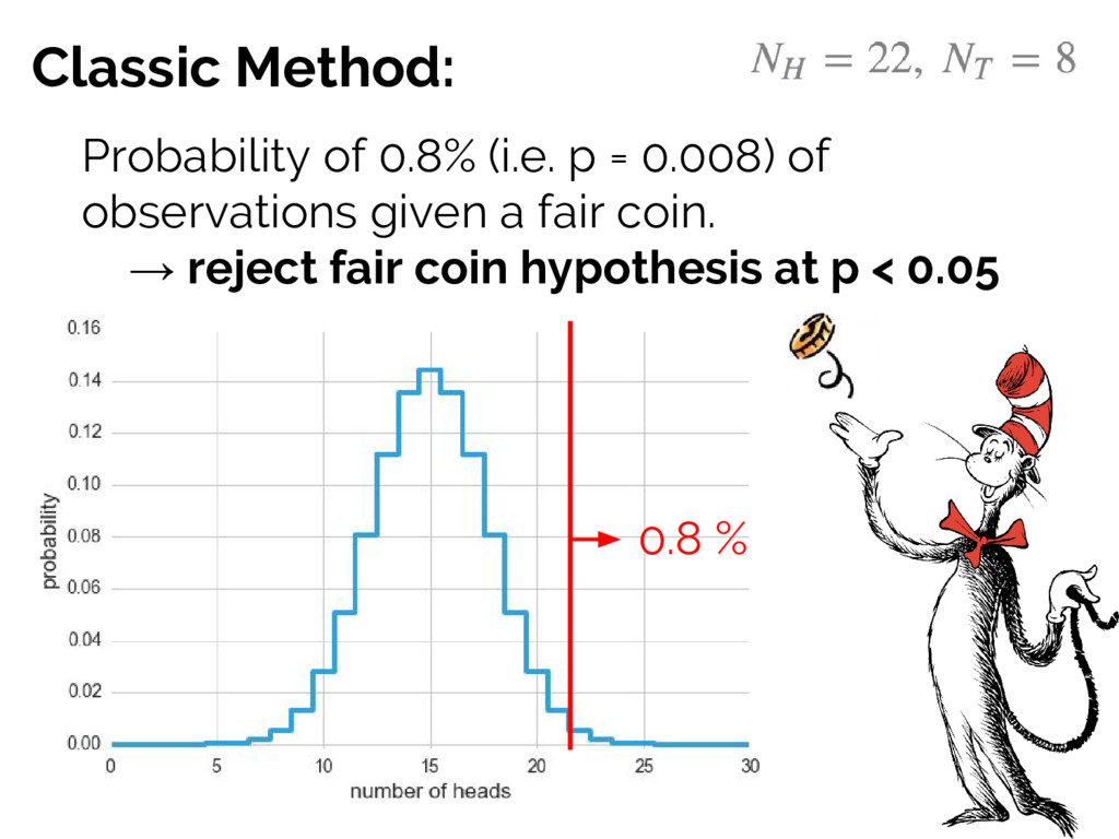
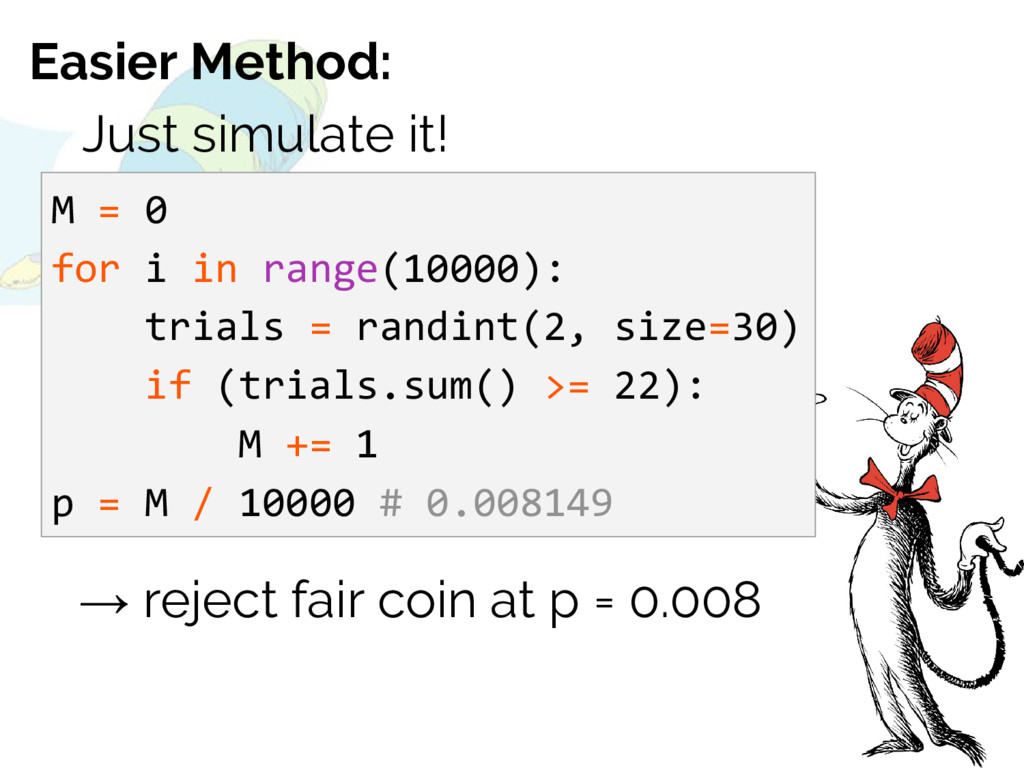
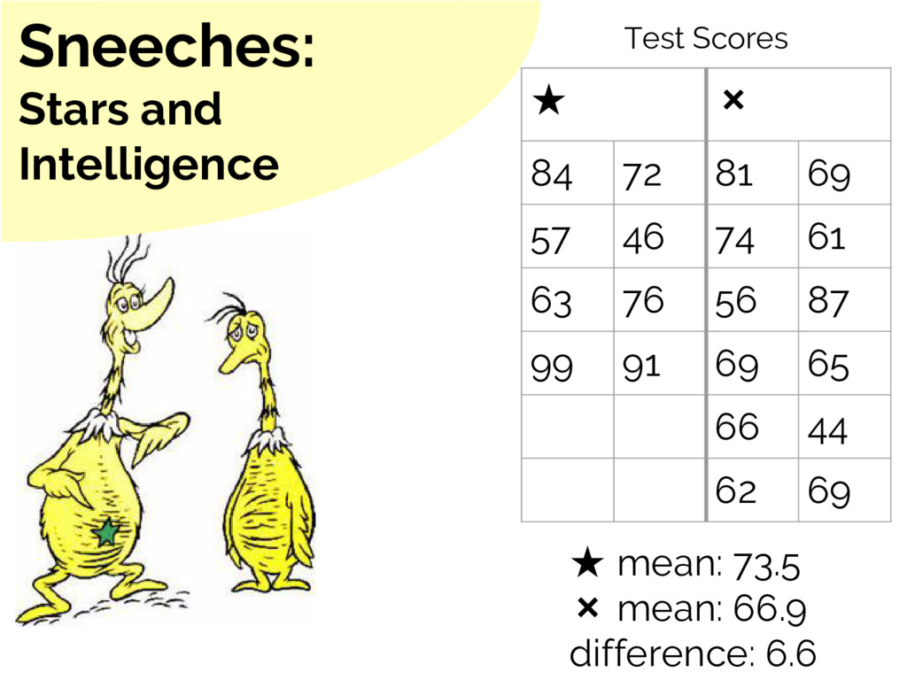
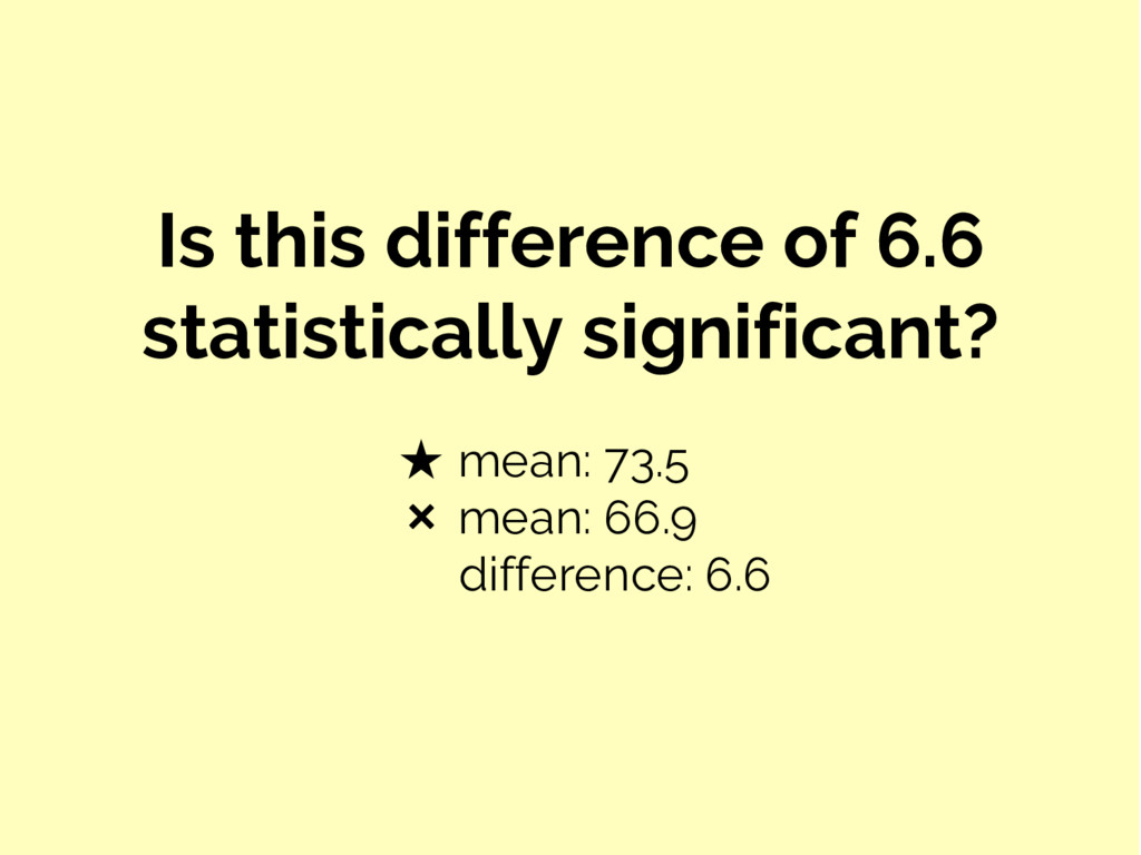
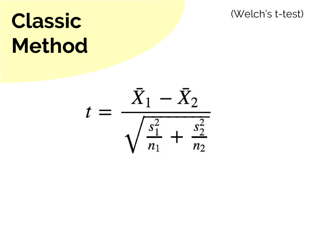
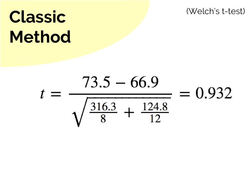
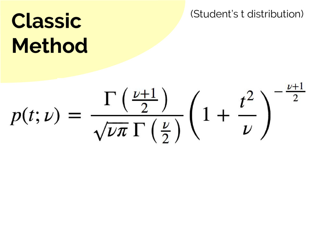
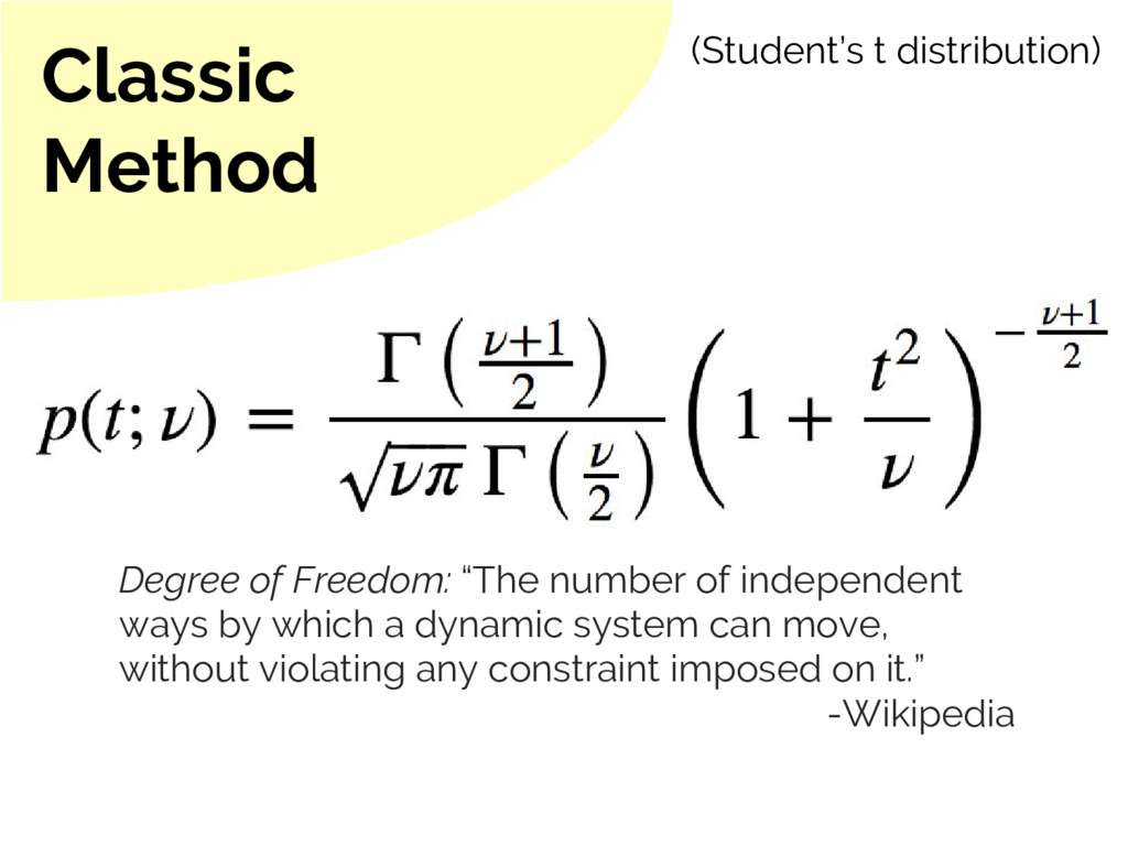
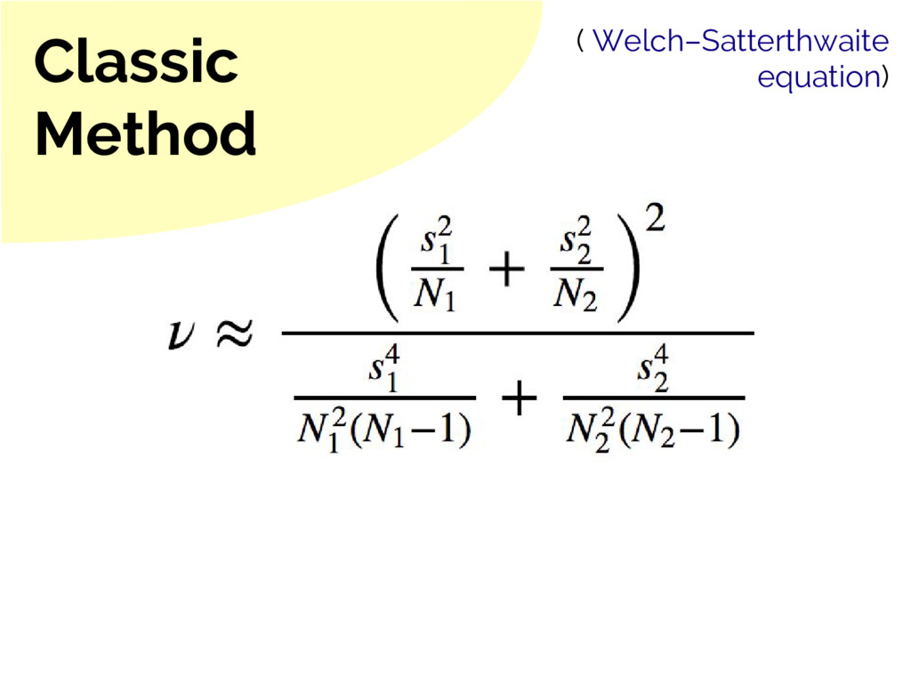
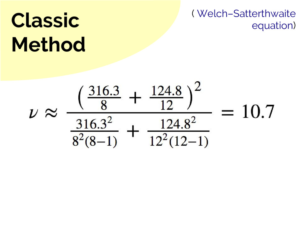
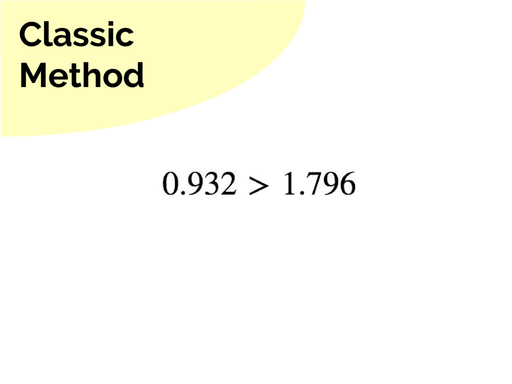
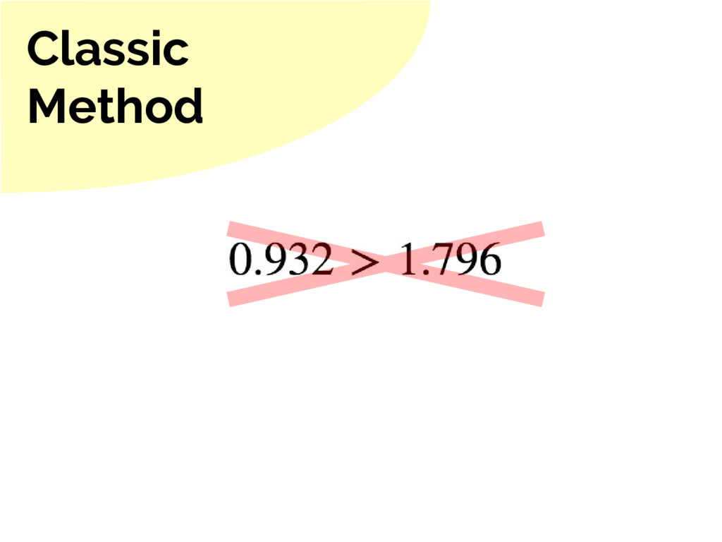
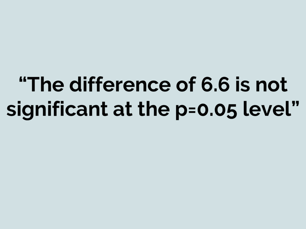
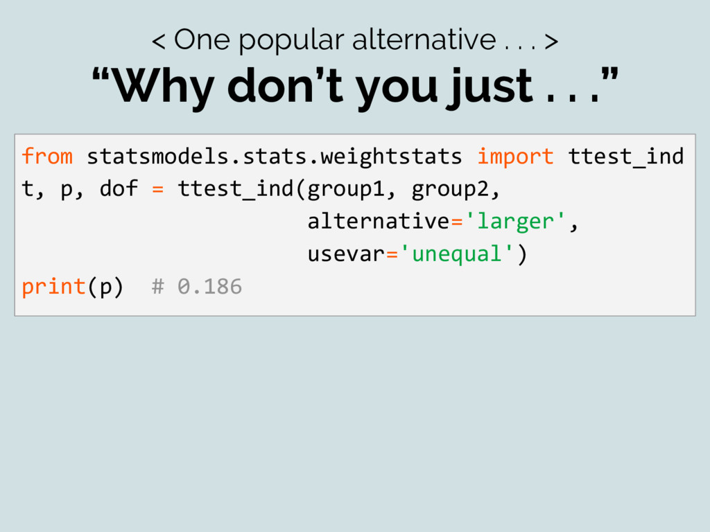
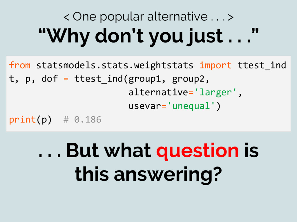
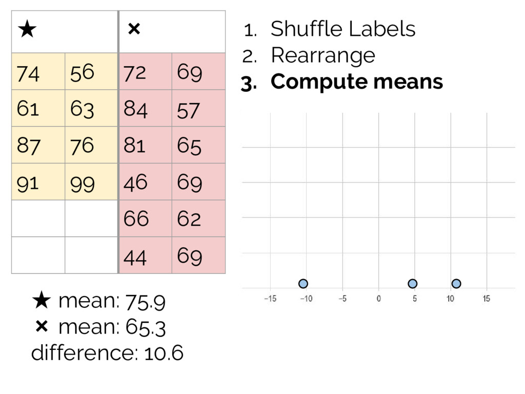
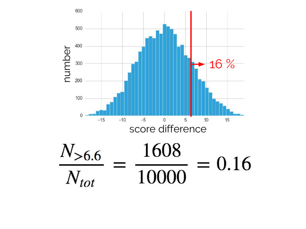
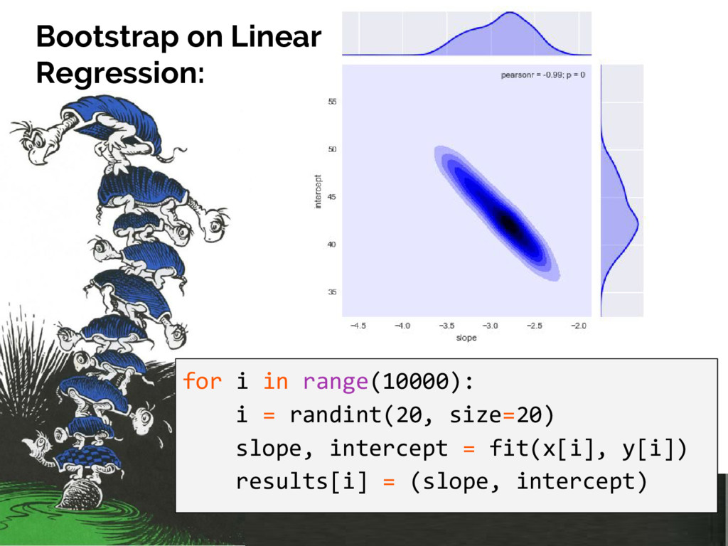
47. < One popular alternative . . . > “Why don’t you just . . .” from statsmodels.stats.weightstats import ttest_ind t, p, dof = ttest_ind(group1, group2, alternative='larger', usevar='unequal') print(p) # 0.186 . . . But what question is this answering?
48. The deep meaning lies in the sampling distribution: Stepping Back... 0.8 % Same principle as the coin example:
49. Let’s use a sampling method instead
50. The Problem: Unlike coin flipping, we don’t have a generative model . . .
51. The Problem: Unlike coin flipping, we don’t have a generative model . . . Solution: Shuffling
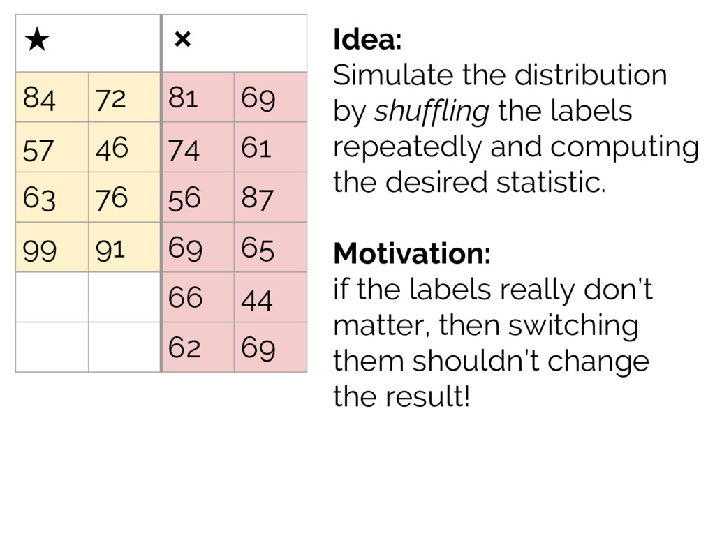
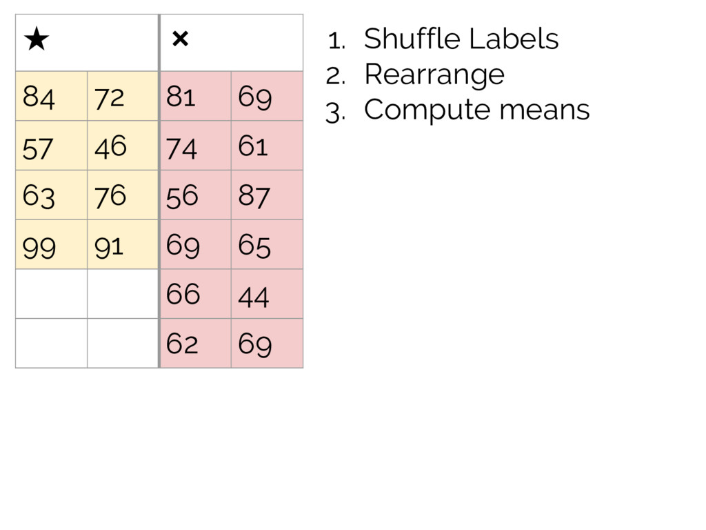
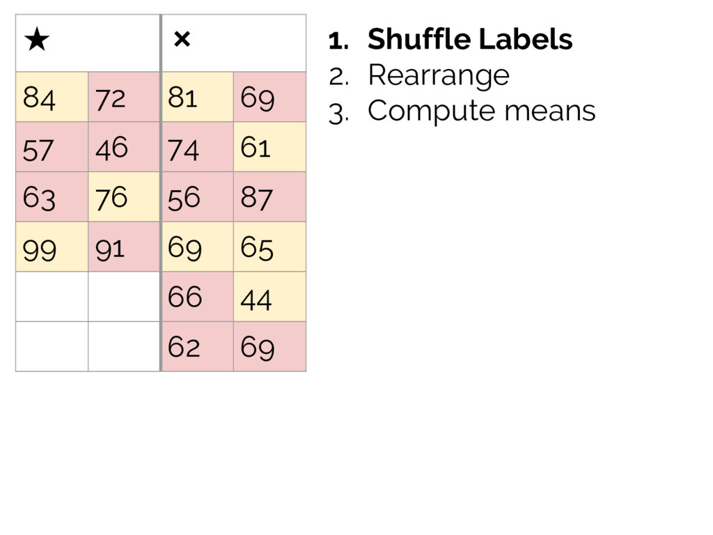
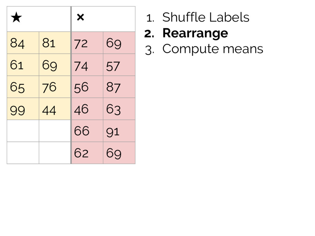
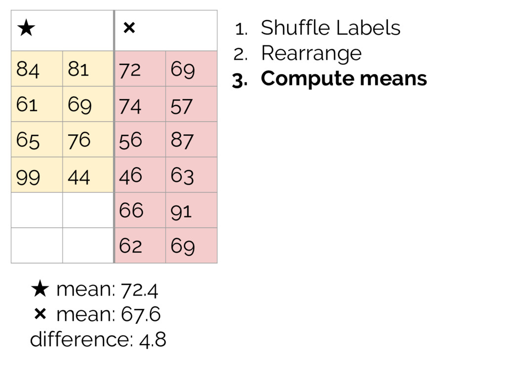
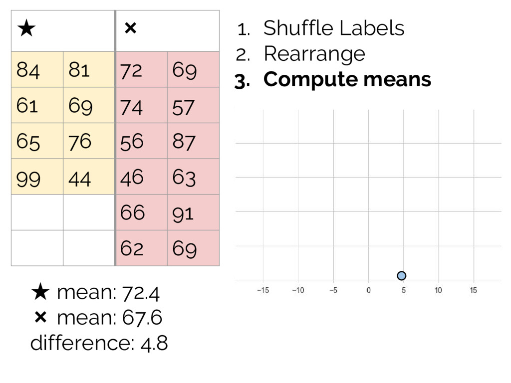
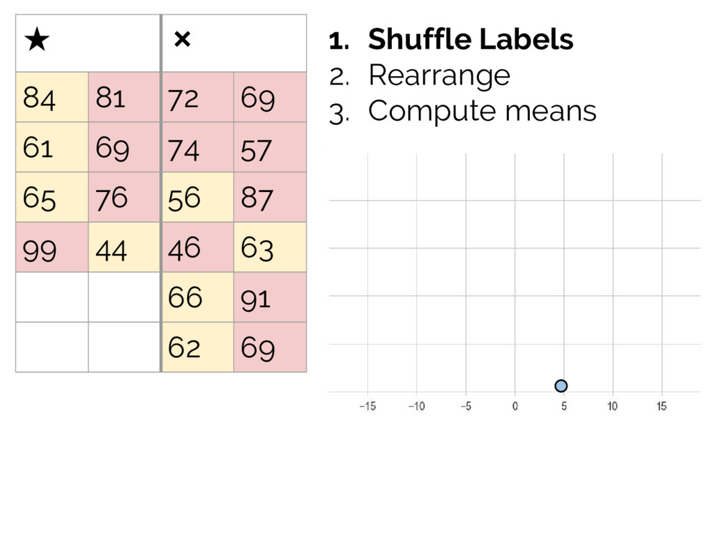
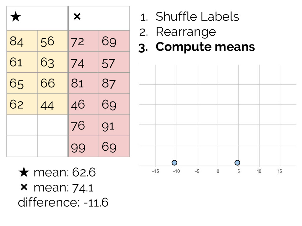
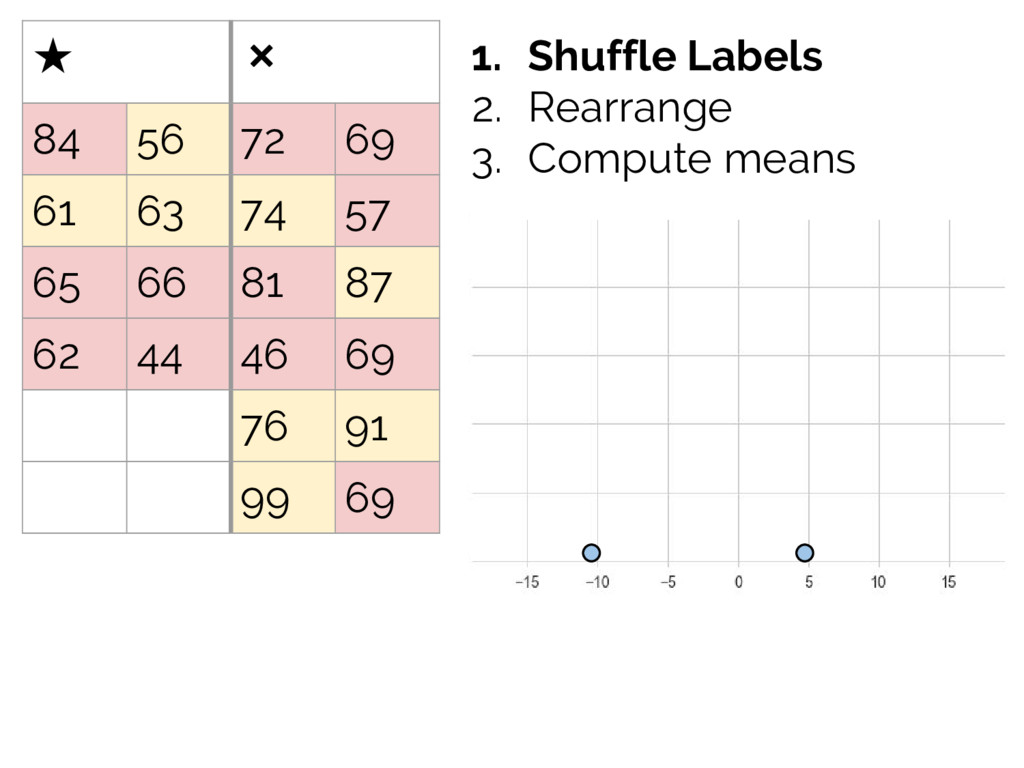
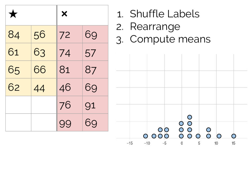
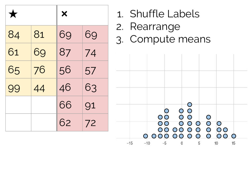
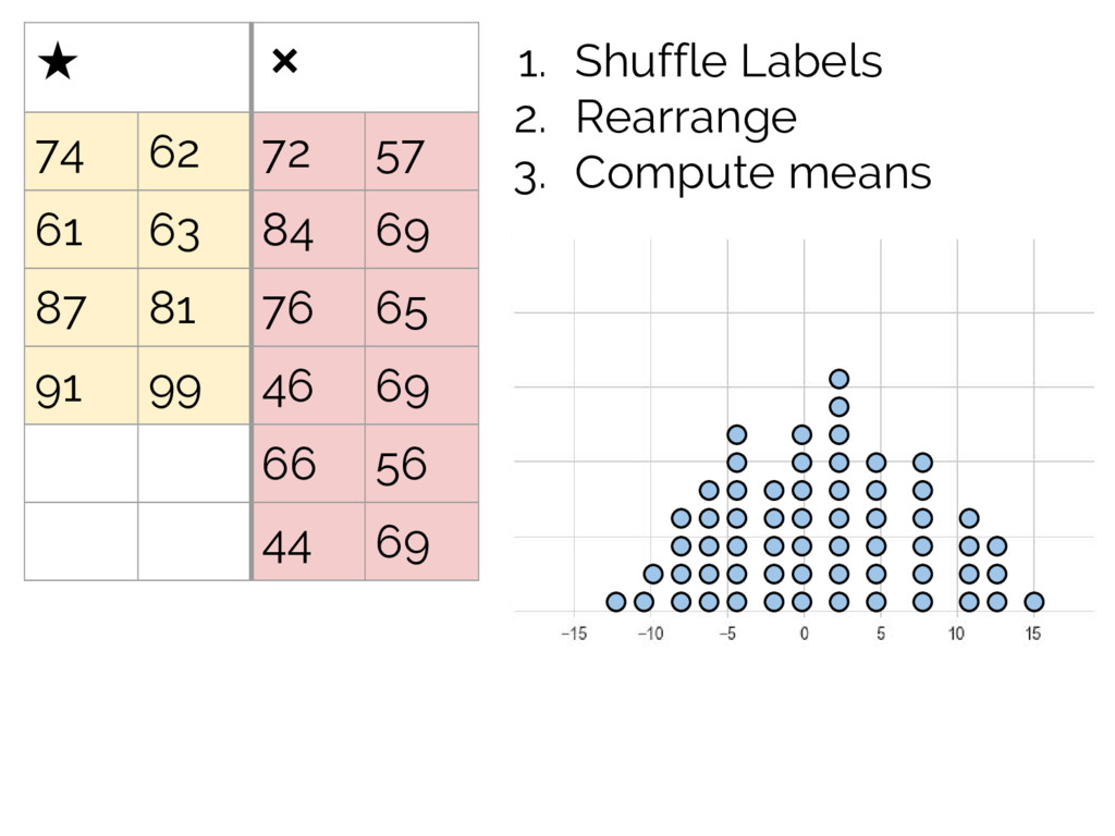
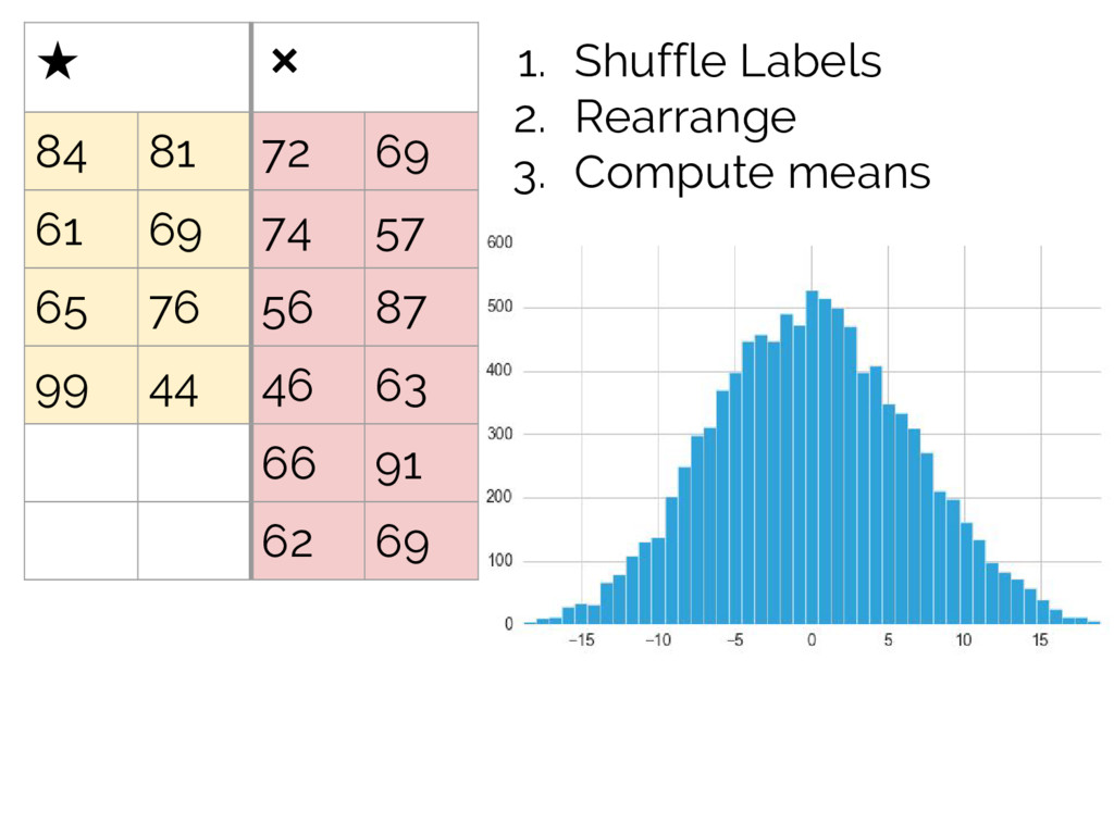
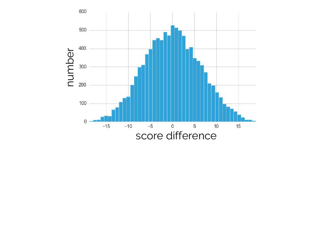
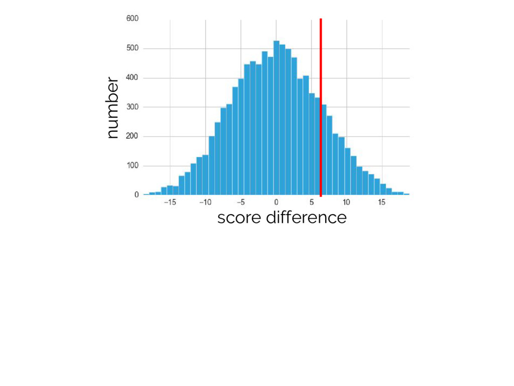
52. ★ ❌ 84 72 81 69 57 46 74 61 63 76 56 87 99 91 69 65 66 44 62 69 Idea: Simulate the distribution by shuffling the labels repeatedly and computing the desired statistic. Motivation: if the labels really don’t matter, then switching them shouldn’t change the result!
53. ★ ❌ 84 72 81 69 57 46 74 61 63 76 56 87 99 91 69 65 66 44 62 69 1. Shuffle Labels 2. Rearrange 3. Compute means
54. ★ ❌ 84 72 81 69 57 46 74 61 63 76 56 87 99 91 69 65 66 44 62 69 1. Shuffle Labels 2. Rearrange 3. Compute means
55. ★ ❌ 84 81 72 69 61 69 74 57 65 76 56 87 99 44 46 63 66 91 62 69 1. Shuffle Labels 2. Rearrange 3. Compute means
56. ★ ❌ 84 81 72 69 61 69 74 57 65 76 56 87 99 44 46 63 66 91 62 69 ★ mean: 72.4 ❌ mean: 67.6 difference: 4.8 1. Shuffle Labels 2. Rearrange 3. Compute means
57. ★ ❌ 84 81 72 69 61 69 74 57 65 76 56 87 99 44 46 63 66 91 62 69 ★ mean: 72.4 ❌ mean: 67.6 difference: 4.8 1. Shuffle Labels 2. Rearrange 3. Compute means
58. ★ ❌ 84 81 72 69 61 69 74 57 65 76 56 87 99 44 46 63 66 91 62 69 1. Shuffle Labels 2. Rearrange 3. Compute means
59. ★ ❌ 84 56 72 69 61 63 74 57 65 66 81 87 62 44 46 69 76 91 99 69 ★ mean: 62.6 ❌ mean: 74.1 difference: -11.6 1. Shuffle Labels 2. Rearrange 3. Compute means
60. ★ ❌ 84 56 72 69 61 63 74 57 65 66 81 87 62 44 46 69 76 91 99 69 1. Shuffle Labels 2. Rearrange 3. Compute means
61. ★ ❌ 74 56 72 69 61 63 84 57 87 76 81 65 91 99 46 69 66 62 44 69 ★ mean: 75.9 ❌ mean: 65.3 difference: 10.6 1. Shuffle Labels 2. Rearrange 3. Compute means
62. ★ ❌ 84 56 72 69 61 63 74 57 65 66 81 87 62 44 46 69 76 91 99 69 1. Shuffle Labels 2. Rearrange 3. Compute means
63. ★ ❌ 84 81 69 69 61 69 87 74 65 76 56 57 99 44 46 63 66 91 62 72 1. Shuffle Labels 2. Rearrange 3. Compute means
64. 1. Shuffle Labels 2. Rearrange 3. Compute means ★ ❌ 74 62 72 57 61 63 84 69 87 81 76 65 91 99 46 69 66 56 44 69
65. 1. Shuffle Labels 2. Rearrange 3. Compute means ★ ❌ 84 81 72 69 61 69 74 57 65 76 56 87 99 44 46 63 66 91 62 69
66. score difference number
67. score difference number
68. 16 % score difference number
69. “A difference of 6.6 is not significant at p = 0.05.” That day, all the Sneetches forgot about stars And whether they had one, or not, upon thars.
70. Notes on Shuffling: - Works when the Null Hypothesis assumes two groups are equivalent - Like all methods, it will only work if your samples are representative – always be careful about selection biases! - Needs care for non-independent trials. Good discussion in Simon’s Resampling: The New Statistics
71. Four Recipes for Hacking Statistics: 1. Direct Simulation 2. Shuffling 3. Bootstrapping 4. Cross Validation
72. Yertle’s Turtle Tower On the far-away island of Sala-ma-Sond, Yertle the Turtle was king of the pond. . .
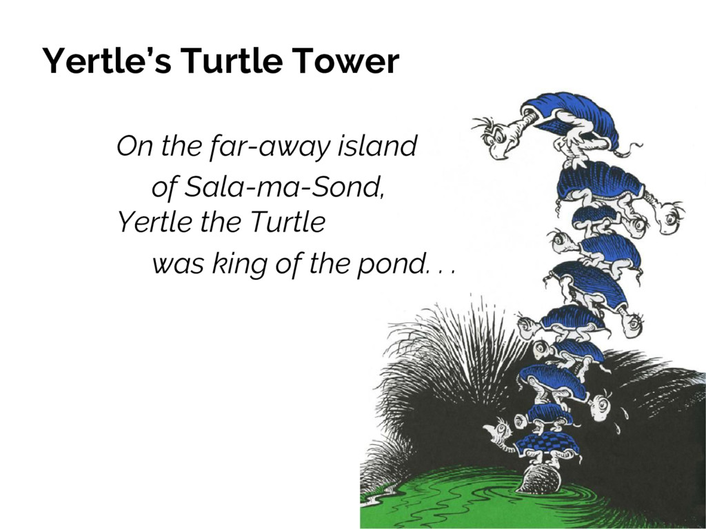
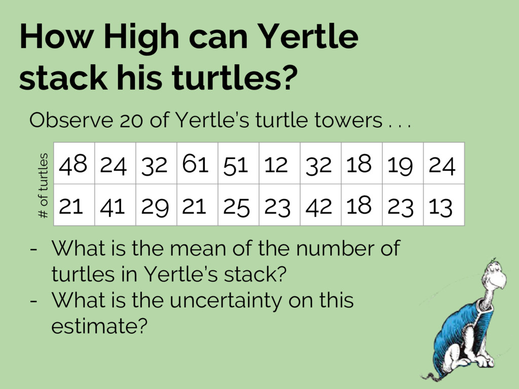
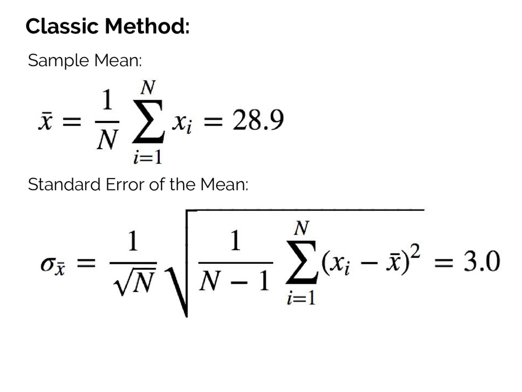
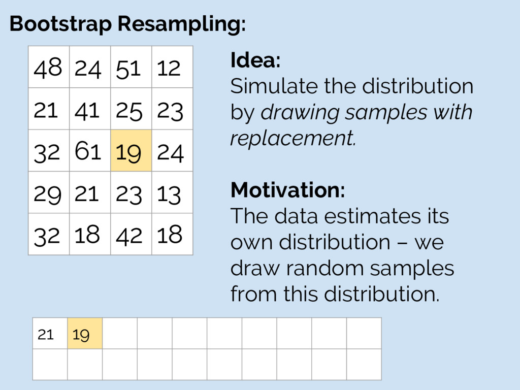
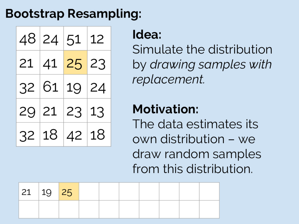
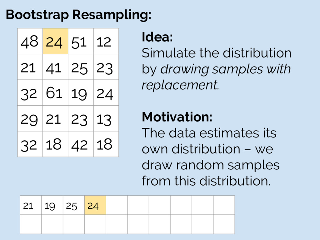
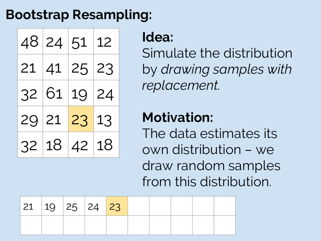
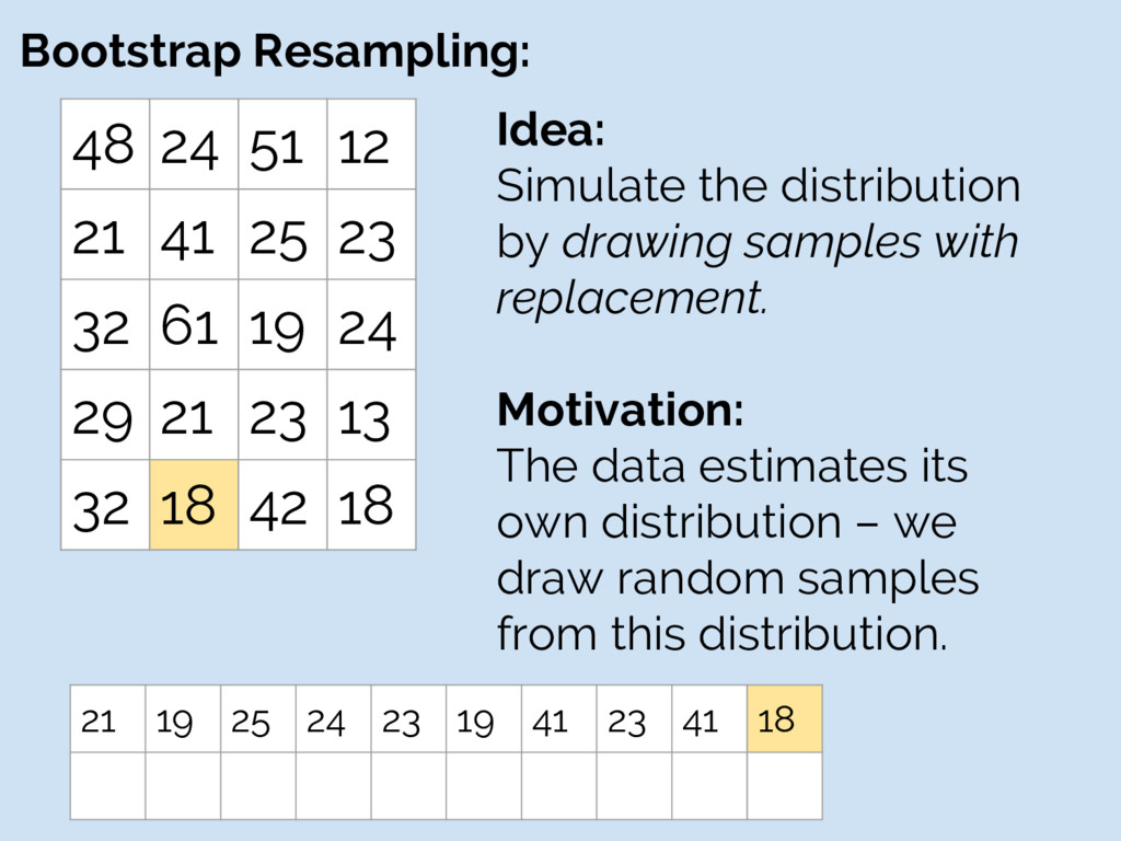
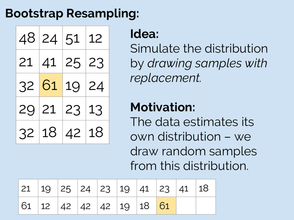
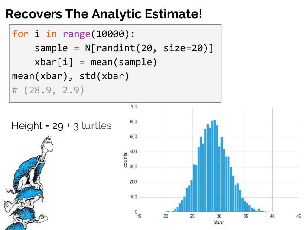
73. How High can Yertle stack his turtles? - What is the mean of the number of turtles in Yertle’s stack? - What is the uncertainty on this estimate? 48 24 32 61 51 12 32 18 19 24 21 41 29 21 25 23 42 18 23 13 Observe 20 of Yertle’s turtle towers . . . # of turtles
74. Classic Method: Sample Mean: Standard Error of the Mean:
75. What assumptions go into these formulae? Can we use sampling instead?
76. Problem: As before, we don’t have a generating model . . .
77. Problem: As before, we don’t have a generating model . . . Solution: Bootstrap Resampling
78. Bootstrap Resampling: 48 24 51 12 21 41 25 23 32 61 19 24 29 21 23 13 32 18 42 18 Idea: Simulate the distribution by drawing samples with replacement. Motivation: The data estimates its own distribution – we draw random samples from this distribution.
79. Bootstrap Resampling: 48 24 51 12 21 41 25 23 32 61 19 24 29 21 23 13 32 18 42 18 Idea: Simulate the distribution by drawing samples with replacement. Motivation: The data estimates its own distribution – we draw random samples from this distribution.
80. Bootstrap Resampling: 48 24 51 12 21 41 25 23 32 61 19 24 29 21 23 13 32 18 42 18 Idea: Simulate the distribution by drawing samples with replacement. Motivation: The data estimates its own distribution – we draw random samples from this distribution. 21
81. Bootstrap Resampling: 48 24 51 12 21 41 25 23 32 61 19 24 29 21 23 13 32 18 42 18 Idea: Simulate the distribution by drawing samples with replacement. Motivation: The data estimates its own distribution – we draw random samples from this distribution. 21 19
82. Bootstrap Resampling: 48 24 51 12 21 41 25 23 32 61 19 24 29 21 23 13 32 18 42 18 Idea: Simulate the distribution by drawing samples with replacement. Motivation: The data estimates its own distribution – we draw random samples from this distribution. 21 19 25
83. Bootstrap Resampling: 48 24 51 12 21 41 25 23 32 61 19 24 29 21 23 13 32 18 42 18 Idea: Simulate the distribution by drawing samples with replacement. Motivation: The data estimates its own distribution – we draw random samples from this distribution. 21 19 25 24
84. Bootstrap Resampling: 48 24 51 12 21 41 25 23 32 61 19 24 29 21 23 13 32 18 42 18 Idea: Simulate the distribution by drawing samples with replacement. Motivation: The data estimates its own distribution – we draw random samples from this distribution. 21 19 25 24 23
85. Bootstrap Resampling: 48 24 51 12 21 41 25 23 32 61 19 24 29 21 23 13 32 18 42 18 Idea: Simulate the distribution by drawing samples with replacement. Motivation: The data estimates its own distribution – we draw random samples from this distribution. 21 19 25 24 23 19
86. Bootstrap Resampling: 48 24 51 12 21 41 25 23 32 61 19 24 29 21 23 13 32 18 42 18 Idea: Simulate the distribution by drawing samples with replacement. Motivation: The data estimates its own distribution – we draw random samples from this distribution. 21 19 25 24 23 19 41
87. Bootstrap Resampling: 48 24 51 12 21 41 25 23 32 61 19 24 29 21 23 13 32 18 42 18 Idea: Simulate the distribution by drawing samples with replacement. Motivation: The data estimates its own distribution – we draw random samples from this distribution. 21 19 25 24 23 19 41 23
88. Bootstrap Resampling: 48 24 51 12 21 41 25 23 32 61 19 24 29 21 23 13 32 18 42 18 Idea: Simulate the distribution by drawing samples with replacement. Motivation: The data estimates its own distribution – we draw random samples from this distribution. 21 19 25 24 23 19 41 23 41
89. Bootstrap Resampling: 48 24 51 12 21 41 25 23 32 61 19 24 29 21 23 13 32 18 42 18 Idea: Simulate the distribution by drawing samples with replacement. Motivation: The data estimates its own distribution – we draw random samples from this distribution. 21 19 25 24 23 19 41 23 41 18
90. Bootstrap Resampling: 48 24 51 12 21 41 25 23 32 61 19 24 29 21 23 13 32 18 42 18 Idea: Simulate the distribution by drawing samples with replacement. Motivation: The data estimates its own distribution – we draw random samples from this distribution. 21 19 25 24 23 19 41 23 41 18 61
91. Bootstrap Resampling: 48 24 51 12 21 41 25 23 32 61 19 24 29 21 23 13 32 18 42 18 Idea: Simulate the distribution by drawing samples with replacement. Motivation: The data estimates its own distribution – we draw random samples from this distribution. 21 19 25 24 23 19 41 23 41 18 61 12
92. Bootstrap Resampling: 48 24 51 12 21 41 25 23 32 61 19 24 29 21 23 13 32 18 42 18 Idea: Simulate the distribution by drawing samples with replacement. Motivation: The data estimates its own distribution – we draw random samples from this distribution. 21 19 25 24 23 19 41 23 41 18 61 12 42
93. Bootstrap Resampling: 48 24 51 12 21 41 25 23 32 61 19 24 29 21 23 13 32 18 42 18 Idea: Simulate the distribution by drawing samples with replacement. Motivation: The data estimates its own distribution – we draw random samples from this distribution. 21 19 25 24 23 19 41 23 41 18 61 12 42 42
94. Bootstrap Resampling: 48 24 51 12 21 41 25 23 32 61 19 24 29 21 23 13 32 18 42 18 Idea: Simulate the distribution by drawing samples with replacement. Motivation: The data estimates its own distribution – we draw random samples from this distribution. 21 19 25 24 23 19 41 23 41 18 61 12 42 42 42
95. Bootstrap Resampling: 48 24 51 12 21 41 25 23 32 61 19 24 29 21 23 13 32 18 42 18 Idea: Simulate the distribution by drawing samples with replacement. Motivation: The data estimates its own distribution – we draw random samples from this distribution. 21 19 25 24 23 19 41 23 41 18 61 12 42 42 42 19
96. Bootstrap Resampling: 48 24 51 12 21 41 25 23 32 61 19 24 29 21 23 13 32 18 42 18 Idea: Simulate the distribution by drawing samples with replacement. Motivation: The data estimates its own distribution – we draw random samples from this distribution. 21 19 25 24 23 19 41 23 41 18 61 12 42 42 42 19 18
97. Bootstrap Resampling: 48 24 51 12 21 41 25 23 32 61 19 24 29 21 23 13 32 18 42 18 Idea: Simulate the distribution by drawing samples with replacement. Motivation: The data estimates its own distribution – we draw random samples from this distribution. 21 19 25 24 23 19 41 23 41 18 61 12 42 42 42 19 18 61
98. Bootstrap Resampling: 48 24 51 12 21 41 25 23 32 61 19 24 29 21 23 13 32 18 42 18 Idea: Simulate the distribution by drawing samples with replacement. Motivation: The data estimates its own distribution – we draw random samples from this distribution. 21 19 25 24 23 19 41 23 41 18 61 12 42 42 42 19 18 61 29
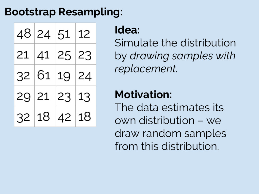
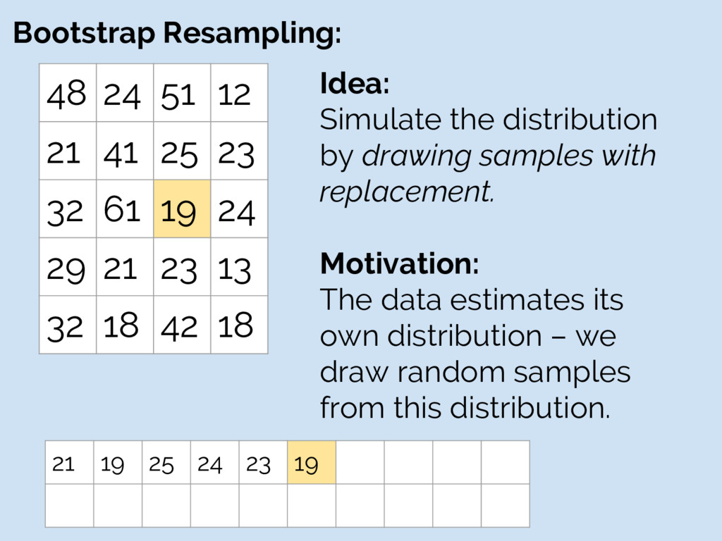
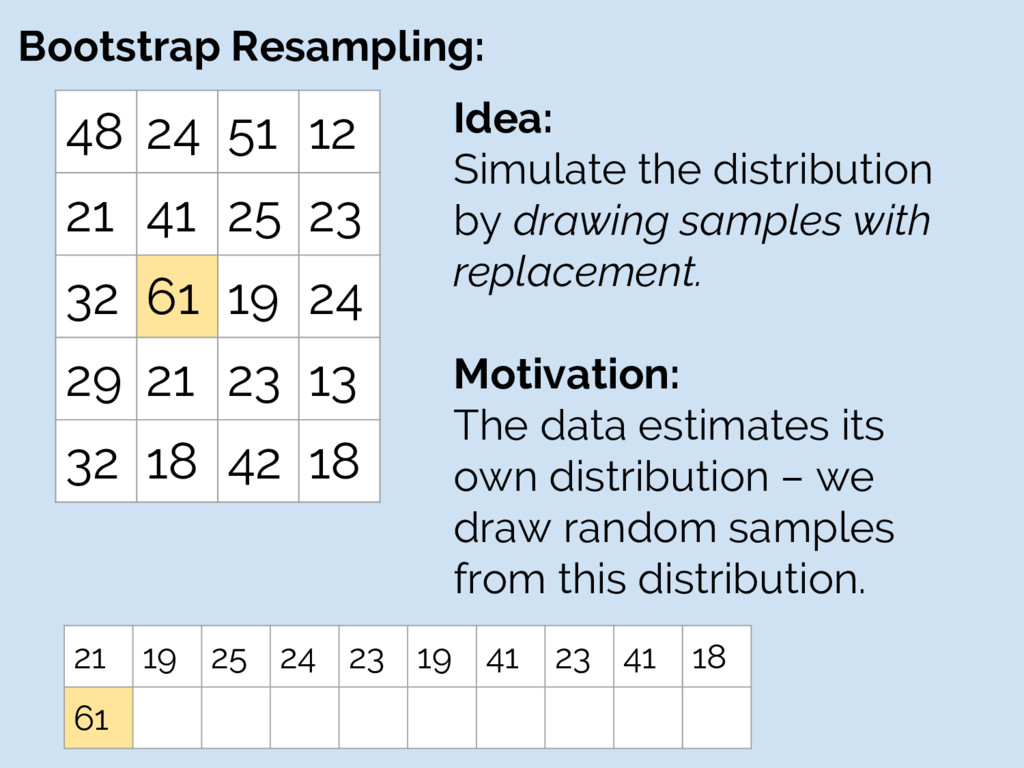
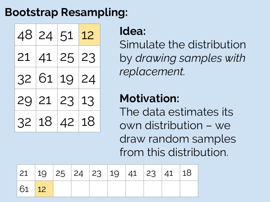
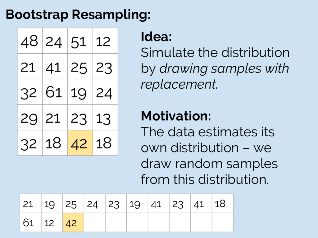
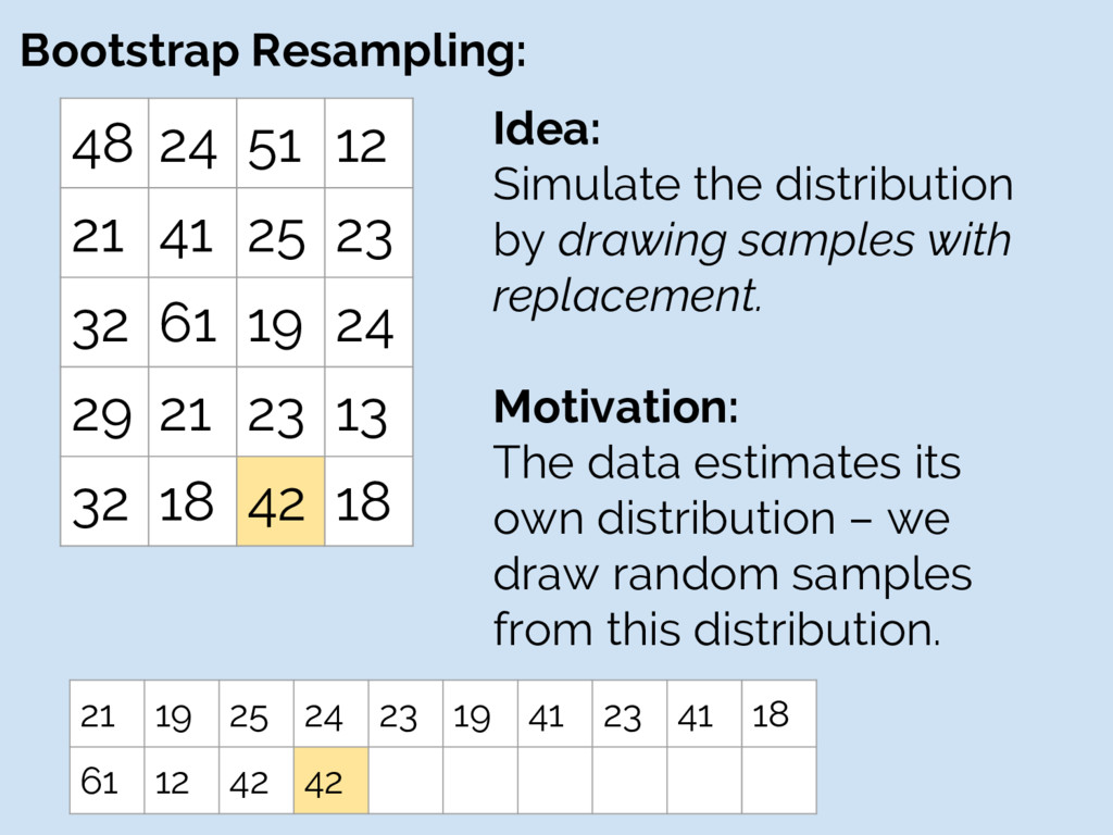
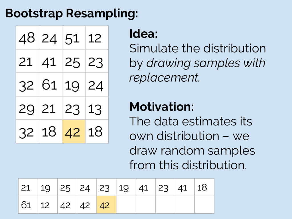
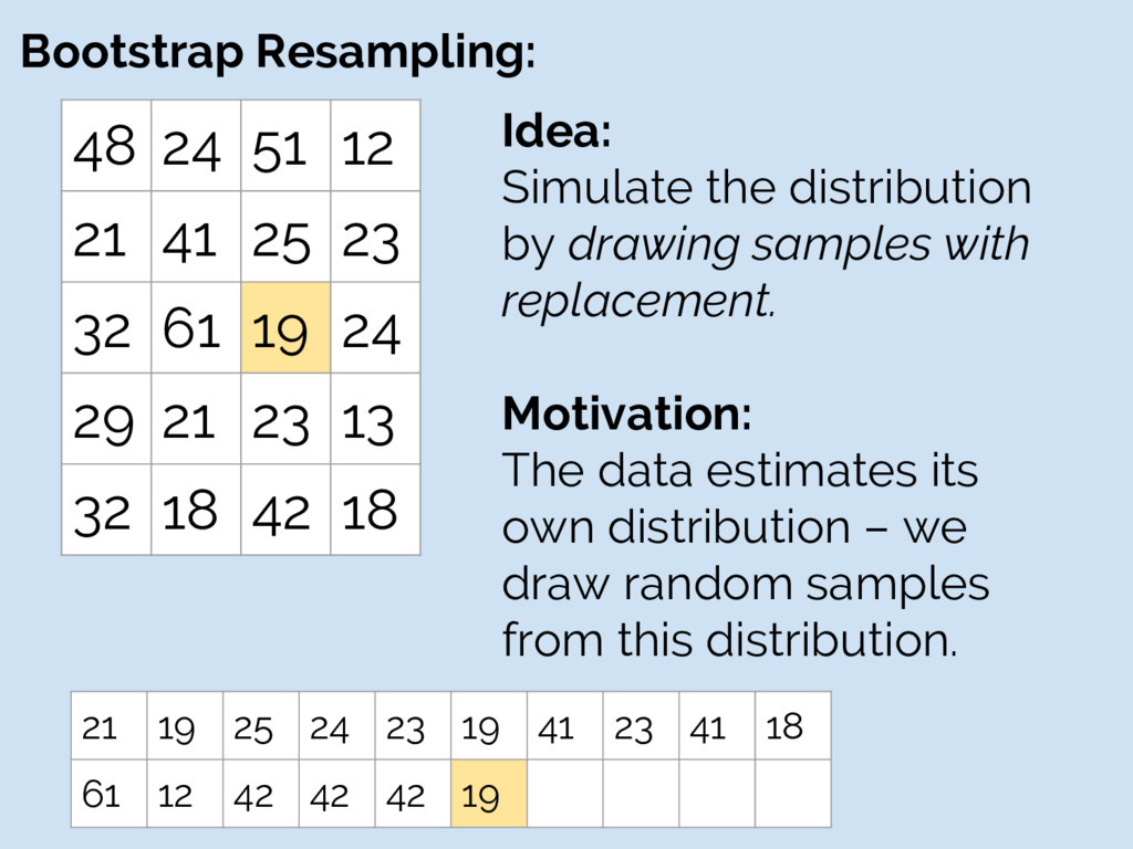
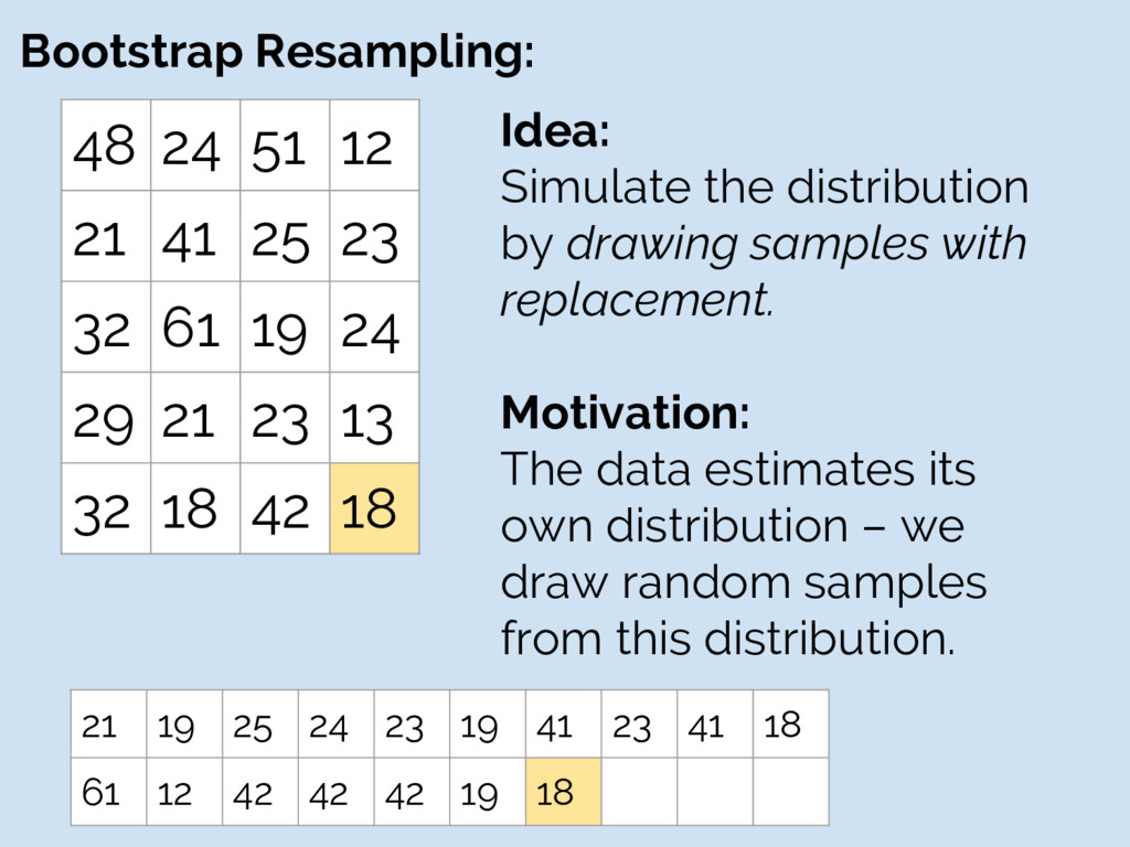
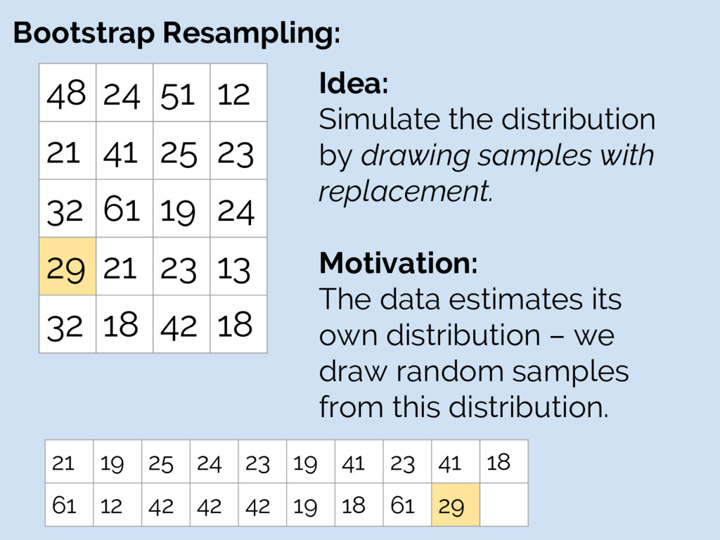
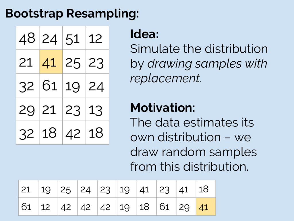
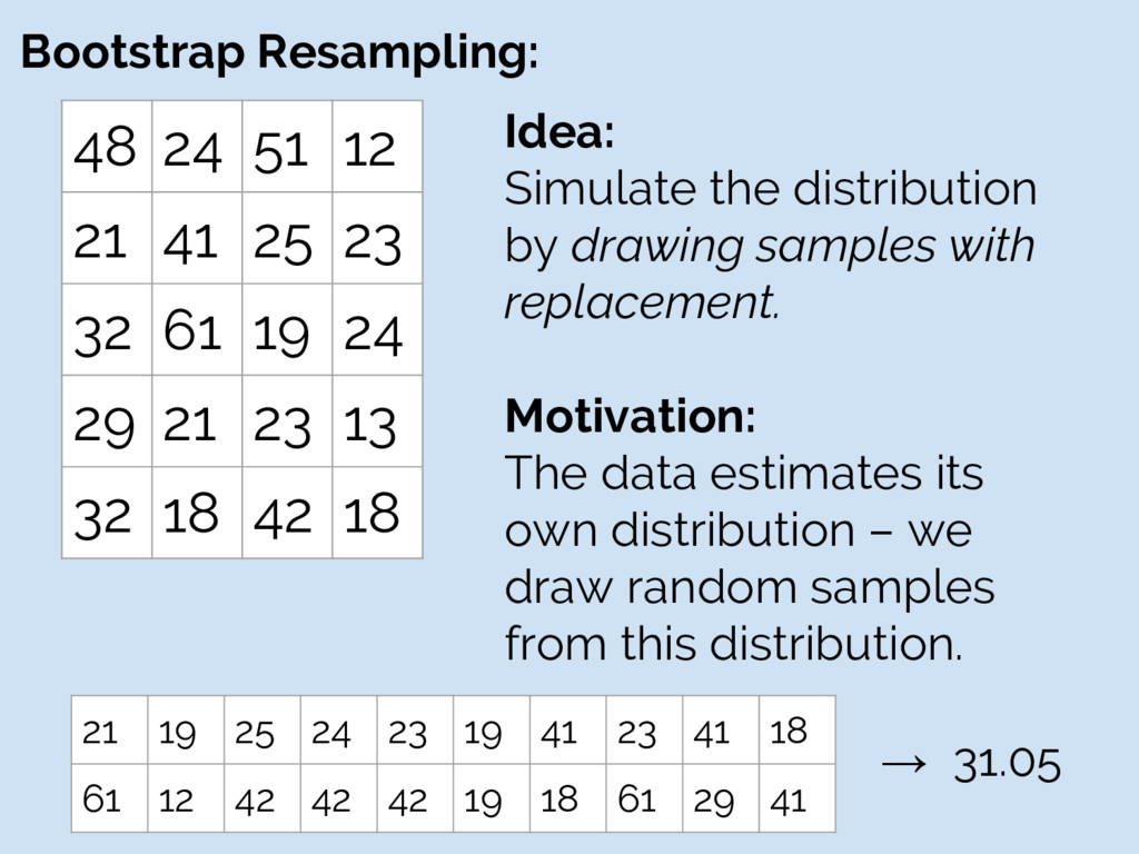
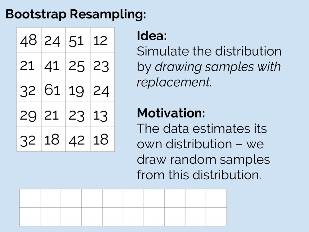
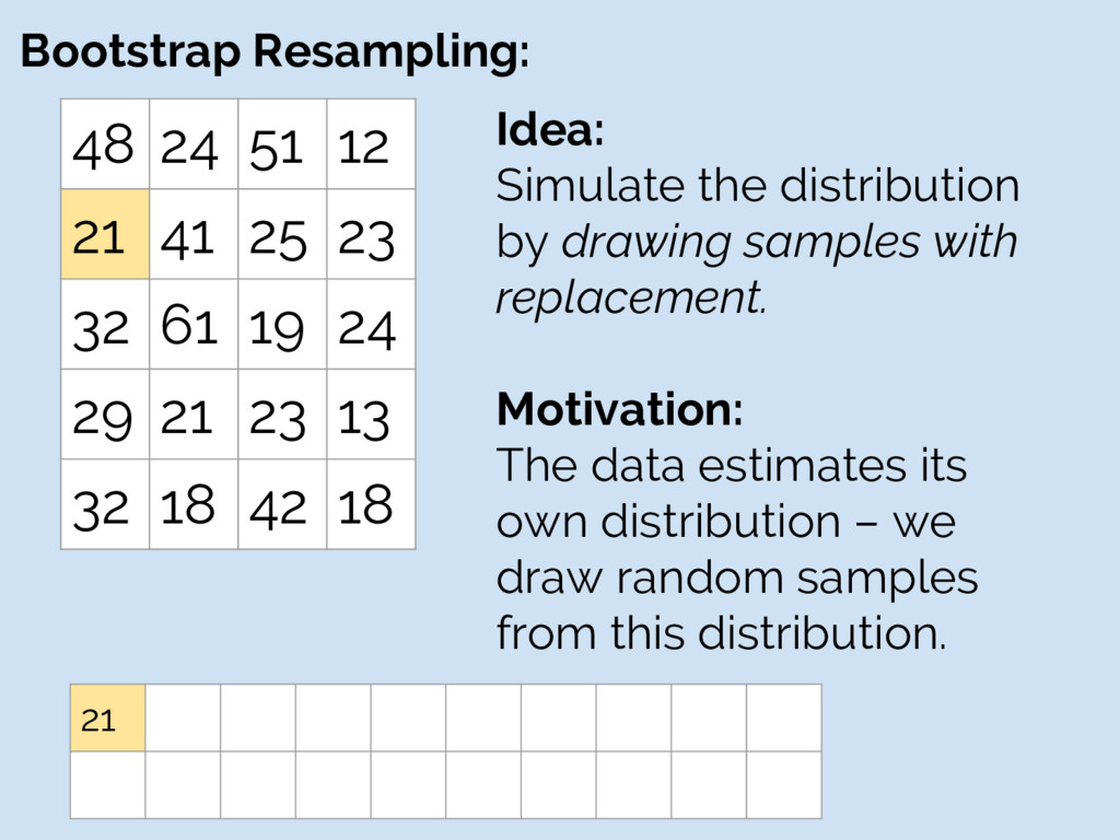
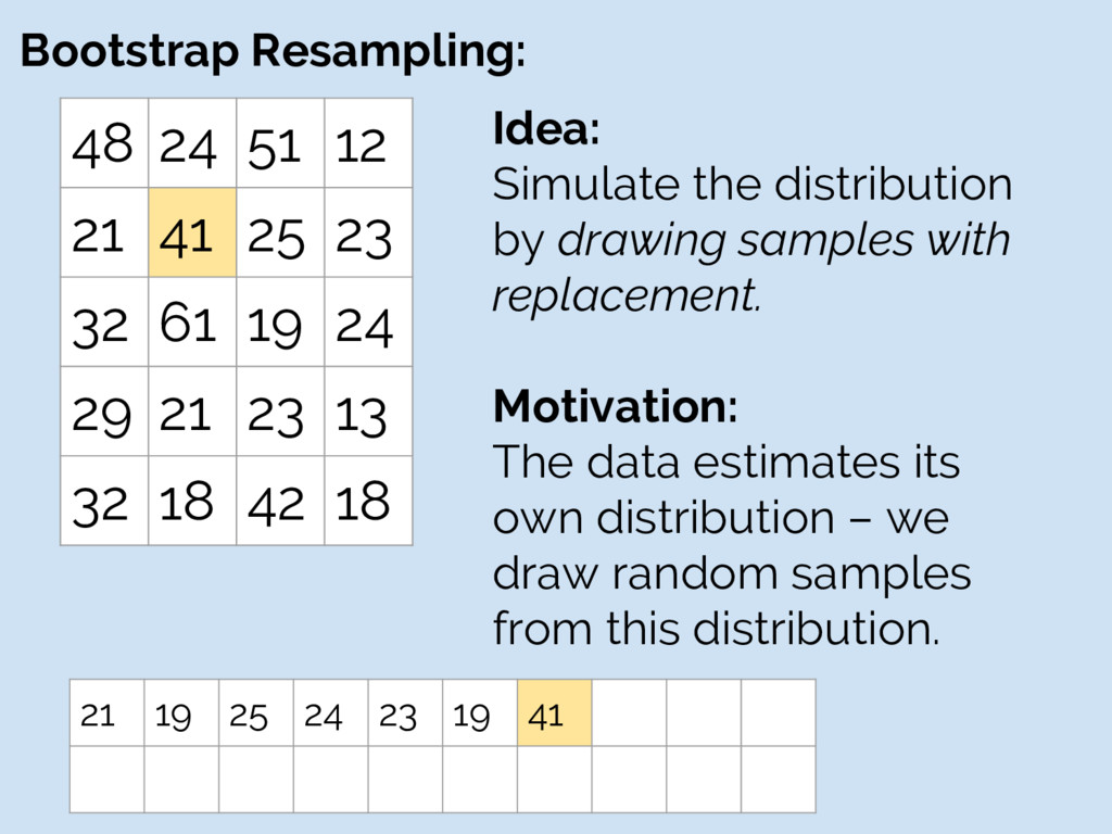
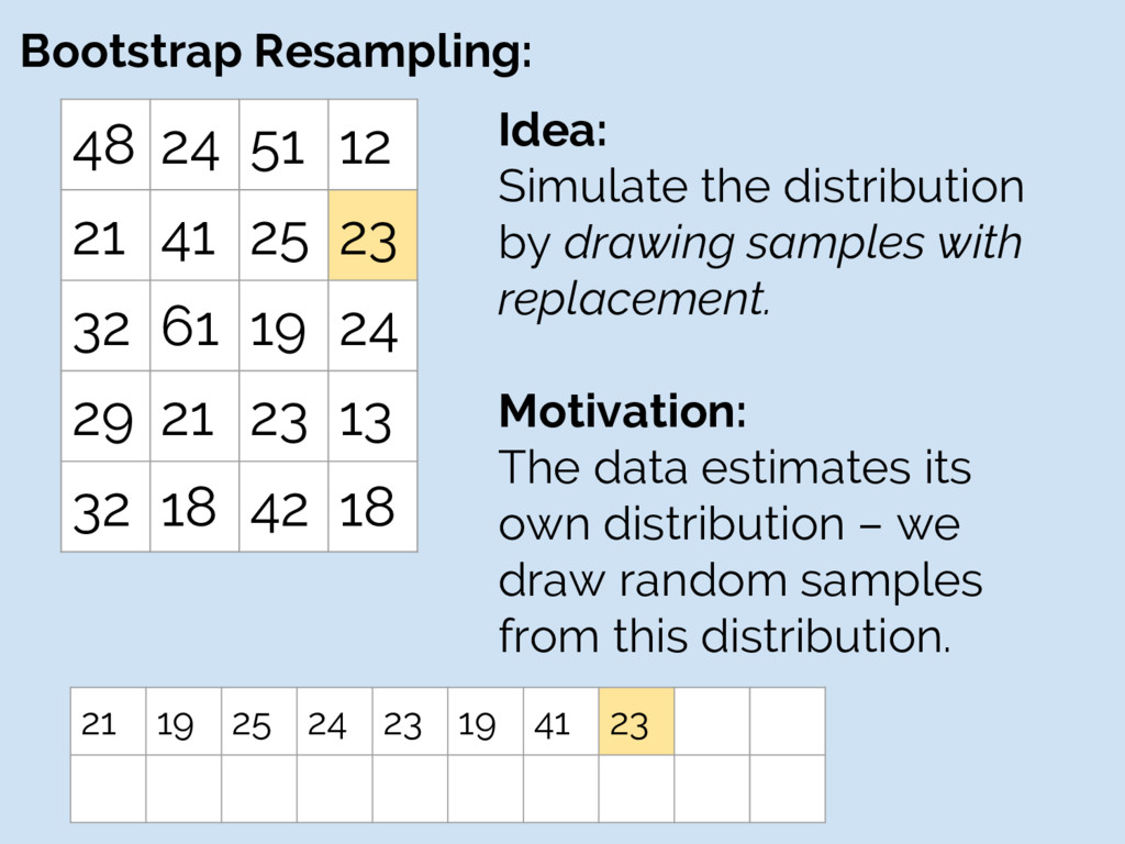
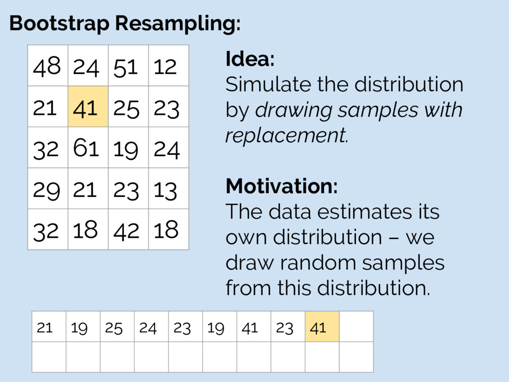
99. Bootstrap Resampling: 48 24 51 12 21 41 25 23 32 61 19 24 29 21 23 13 32 18 42 18 Idea: Simulate the distribution by drawing samples with replacement. Motivation: The data estimates its own distribution – we draw random samples from this distribution. 21 19 25 24 23 19 41 23 41 18 61 12 42 42 42 19 18 61 29 41
100. Bootstrap Resampling: 48 24 51 12 21 41 25 23 32 61 19 24 29 21 23 13 32 18 42 18 Idea: Simulate the distribution by drawing samples with replacement. Motivation: The data estimates its own distribution – we draw random samples from this distribution. 21 19 25 24 23 19 41 23 41 18 61 12 42 42 42 19 18 61 29 41 → 31.05
101. Repeat this several thousand times . . .
102. for i in range(10000): sample = N[randint(20, size=20)] xbar[i] = mean(sample) mean(xbar), std(xbar) # (28.9, 2.9) Recovers The Analytic Estimate! Height = 29 ± 3 turtles
103. Bootstrap sampling can be applied even to more involved statistics
104. Bootstrap on Linear Regression: What is the relationship between speed of wind and the height of the Yertle’s turtle tower?
105. Bootstrap on Linear Regression: for i in range(10000): i = randint(20, size=20) slope, intercept = fit(x[i], y[i]) results[i] = (slope, intercept)
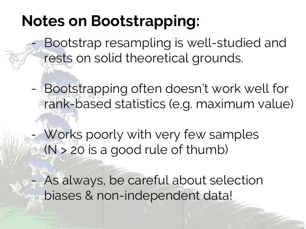
106. Notes on Bootstrapping: - Bootstrap resampling is well-studied and rests on solid theoretical grounds. - Bootstrapping often doesn’t work well for rank-based statistics (e.g. maximum value) - Works poorly with very few samples (N > 20 is a good rule of thumb) - As always, be careful about selection biases & non-independent data!
107. Four Recipes for Hacking Statistics: 1. Direct Simulation 2. Shuffling 3. Bootstrapping 4. Cross Validation
108. Onceler Industries: Sales of Thneeds I'm being quite useful! This thing is a Thneed. A Thneed's a Fine-Something- That-All-People-Need!
109. Thneed sales seem to show a trend with temperature . . .
110. y = a + bx y = a + bx + cx2 But which model is a better fit?
111. y = a + bx y = a + bx + cx2 Can we judge by root-mean- square error? RMS error = 63.0 RMS error = 51.5
112. In general, more flexible models will always have a lower RMS error. y = a + bx y = a + bx + cx2 y = a + bx + cx2 + dx3 y = a + bx + cx2 + dx3 + ex4 y = a + ⋯
113. y = a + bx + cx2 + dx3 + ex4 + fx5 + ⋯ + nx14 RMS error does not tell the whole story.
114. Not to worry: Statistics has figured this out.
115. Classic Method Difference in Mean Squared Error follows chi-square distribution:
116. Classic Method Can estimate degrees of freedom easily because the models are nested . . . Difference in Mean Squared Error follows chi-square distribution:
117. Classic Method Can estimate degrees of freedom easily because the models are nested . . . Difference in Mean Squared Error follows chi-square distribution: Plug in our numbers . . .
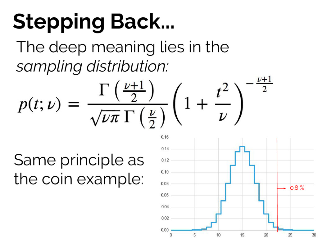
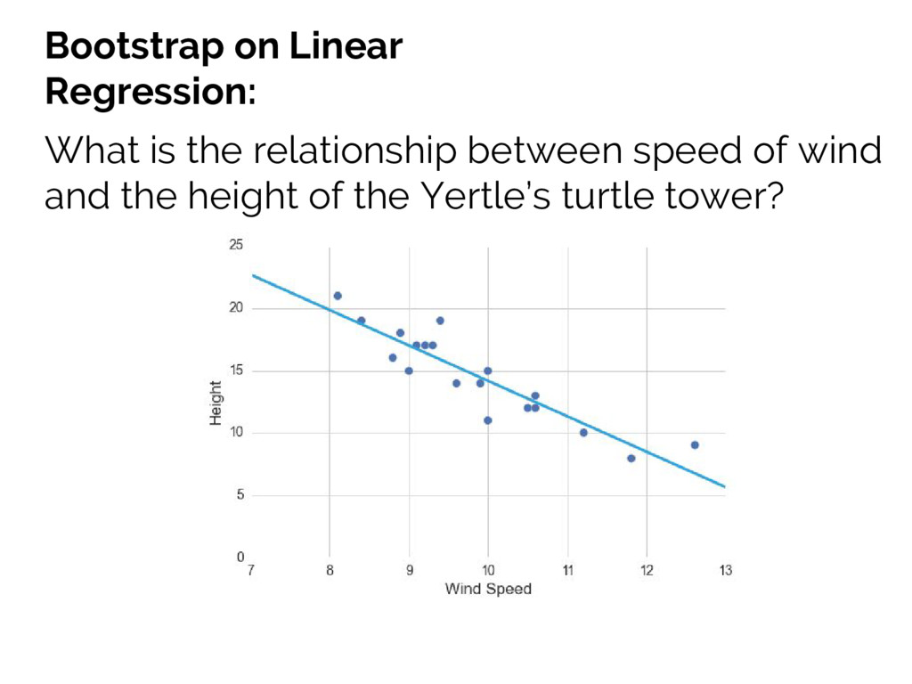
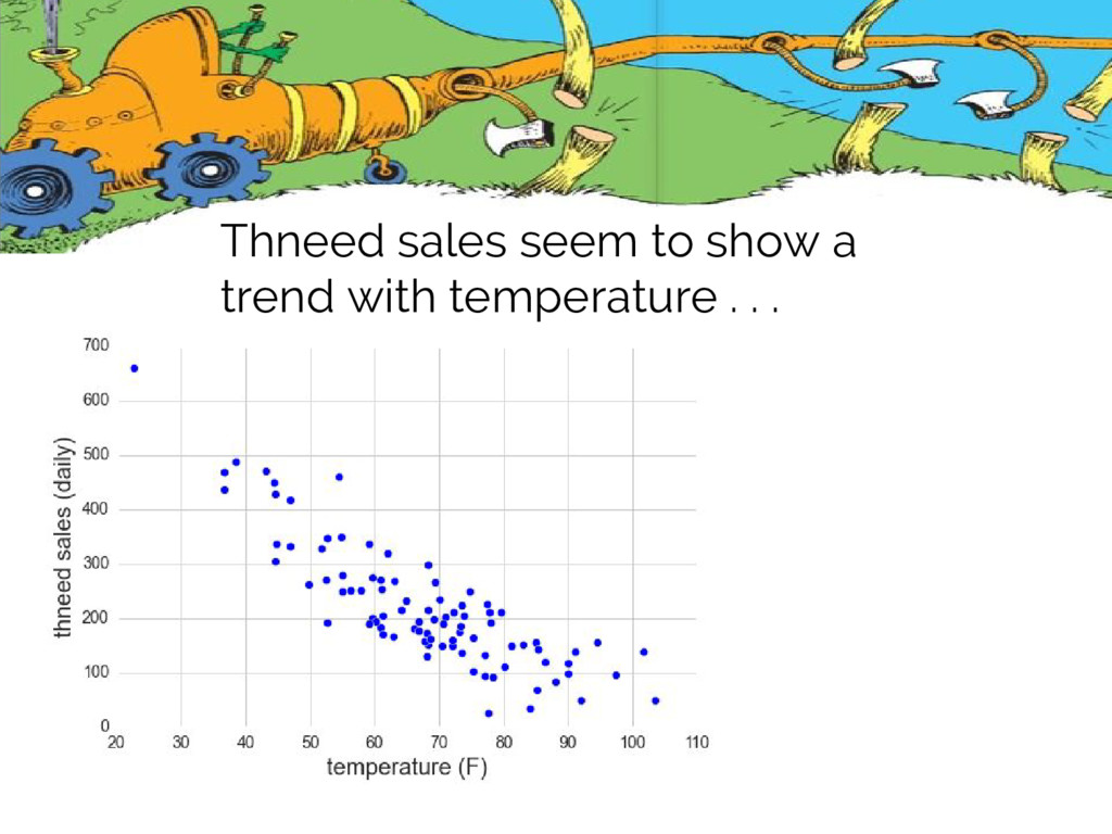
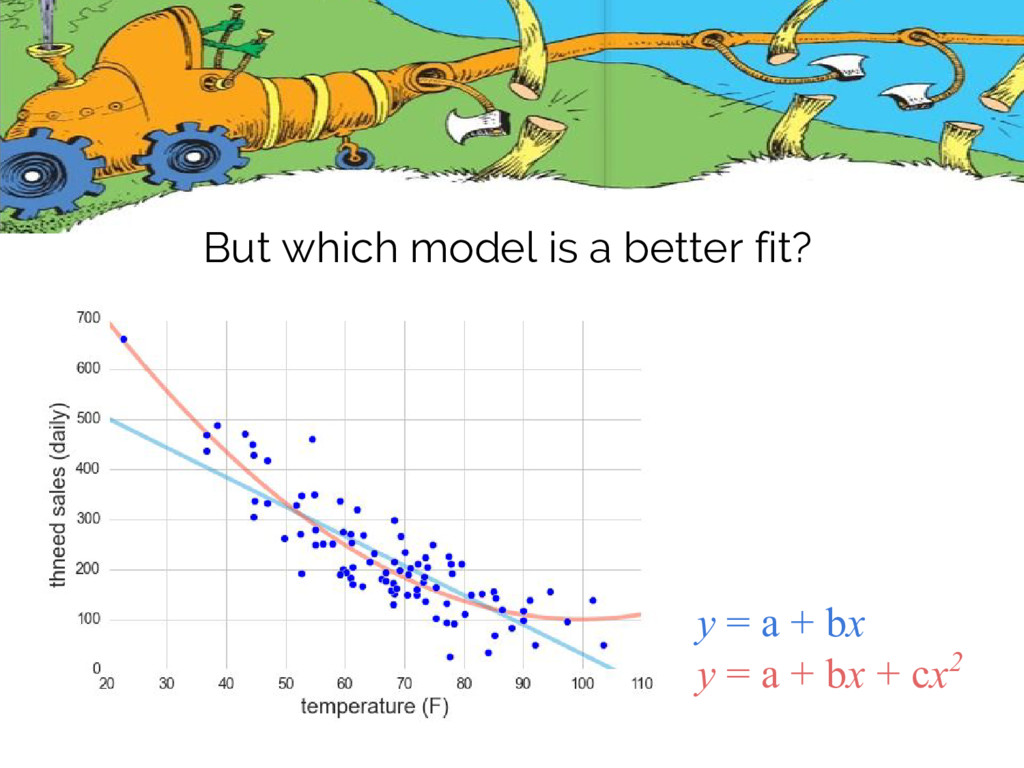
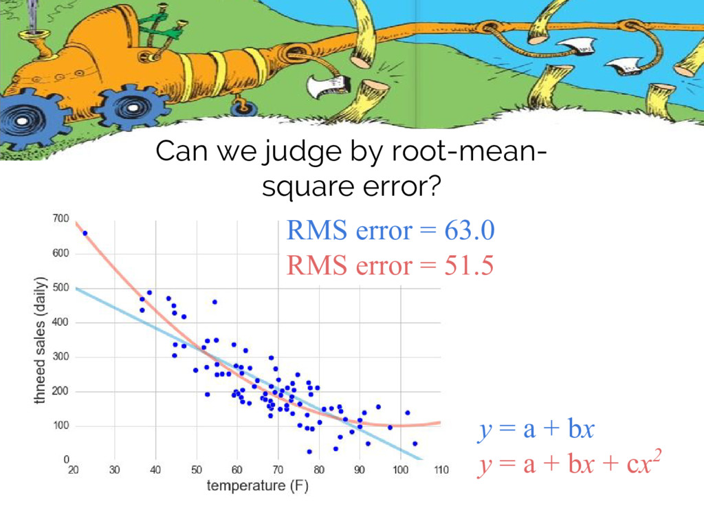
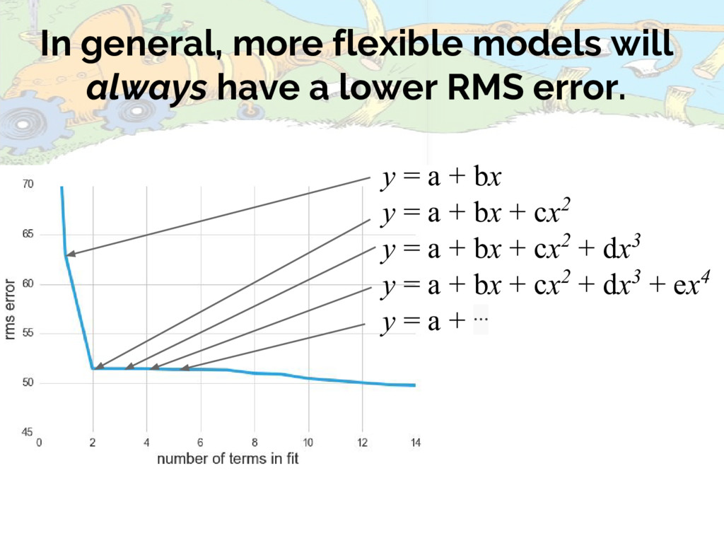
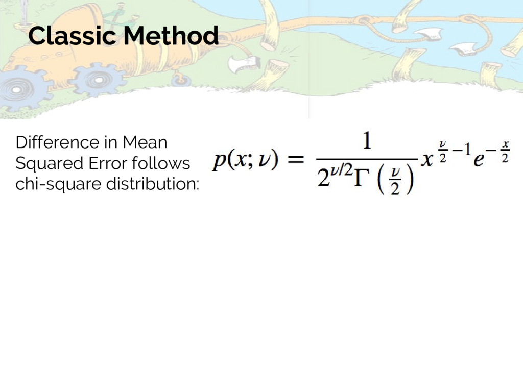
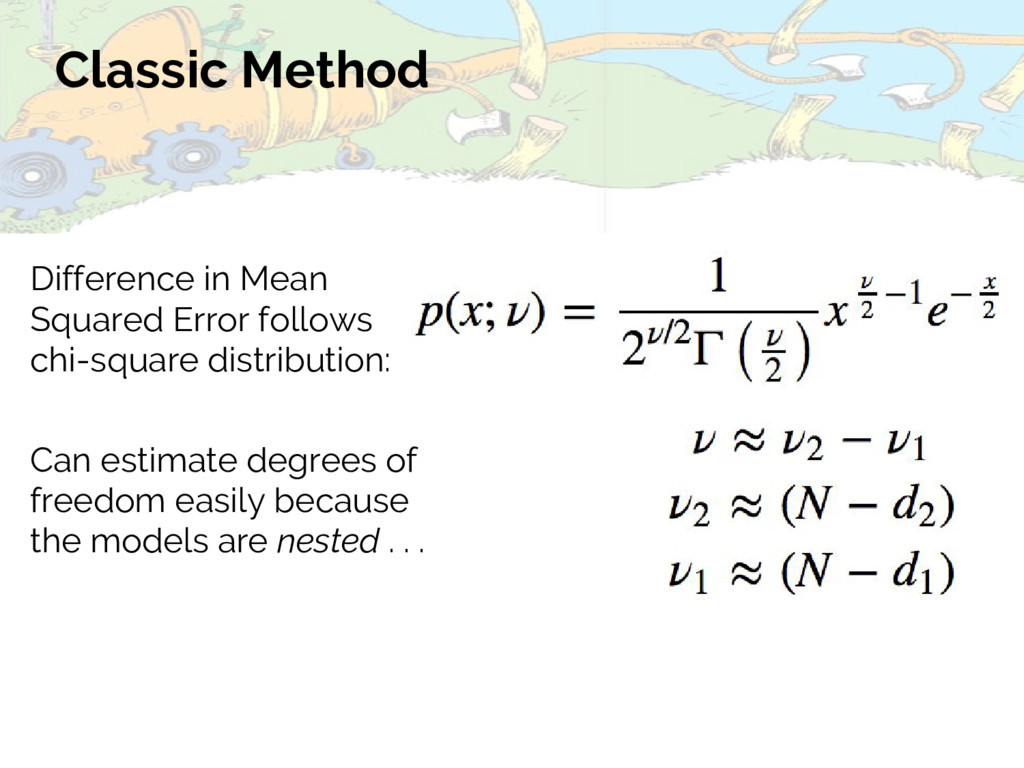
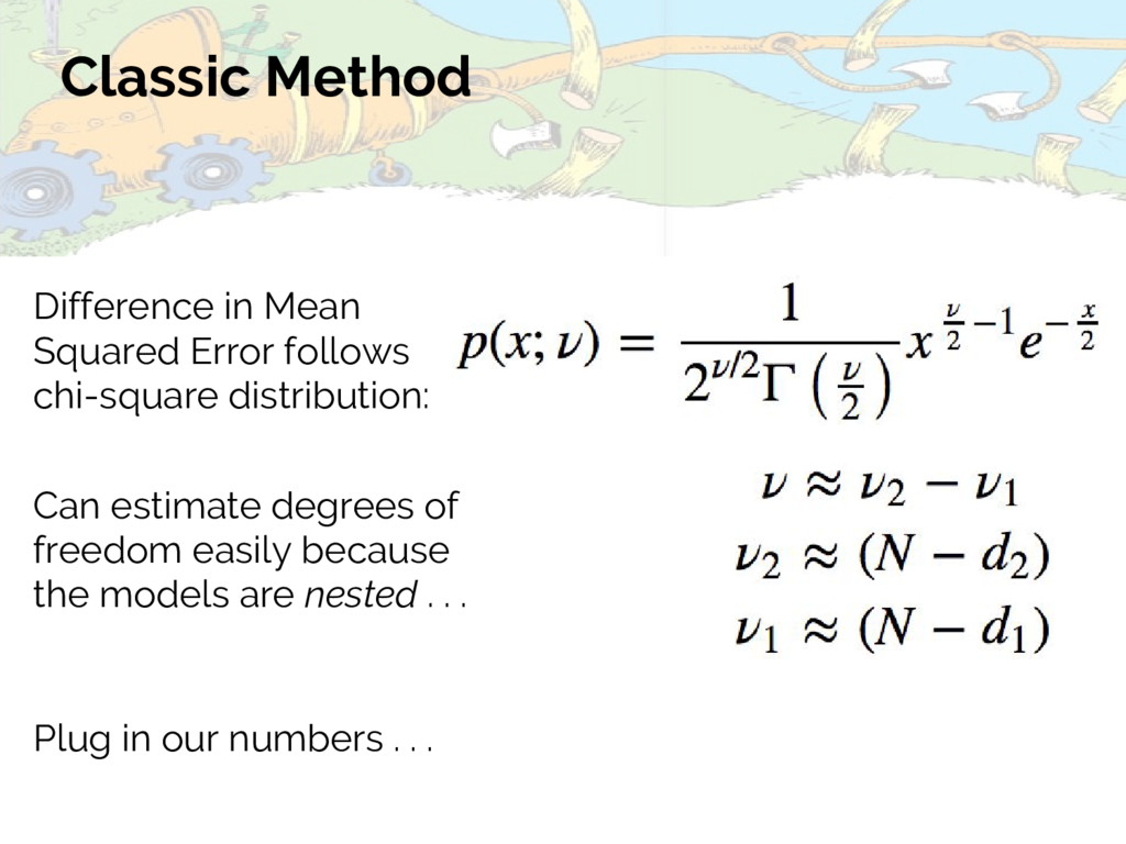
118. Classic Method Can estimate degrees of freedom easily because the models are nested . . . Difference in Mean Squared Error follows chi-square distribution: Plug in our numbers . . . Wait… what question were we trying to answer again?
119. Another Approach: Cross Validation
120. Cross-Validation
121. Cross-Validation 1. Randomly Split data
122. Cross-Validation 1. Randomly Split data
123. Cross-Validation 2. Find the best model for each subset
124. Cross-Validation 3. Compare models across subsets
125. Cross-Validation 3. Compare models across subsets
126. Cross-Validation 3. Compare models across subsets
127. Cross-Validation 3. Compare models across subsets
128. Cross-Validation 4. Compute RMS error for each RMS = 48.9 RMS = 55.1 RMS estimate = 52.1
129. Cross-Validation Repeat for as long as you have patience . . .
130. Cross-Validation 5. Compare cross-validated RMS for models:
131. Cross-Validation Best model minimizes the cross-validated error. 5. Compare cross-validated RMS for models:
132. . . . I biggered the loads of the thneeds I shipped out! I was shipping them forth, to the South, to the East to the West, to the North!
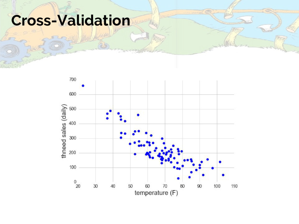
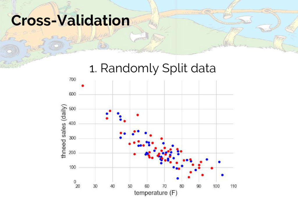
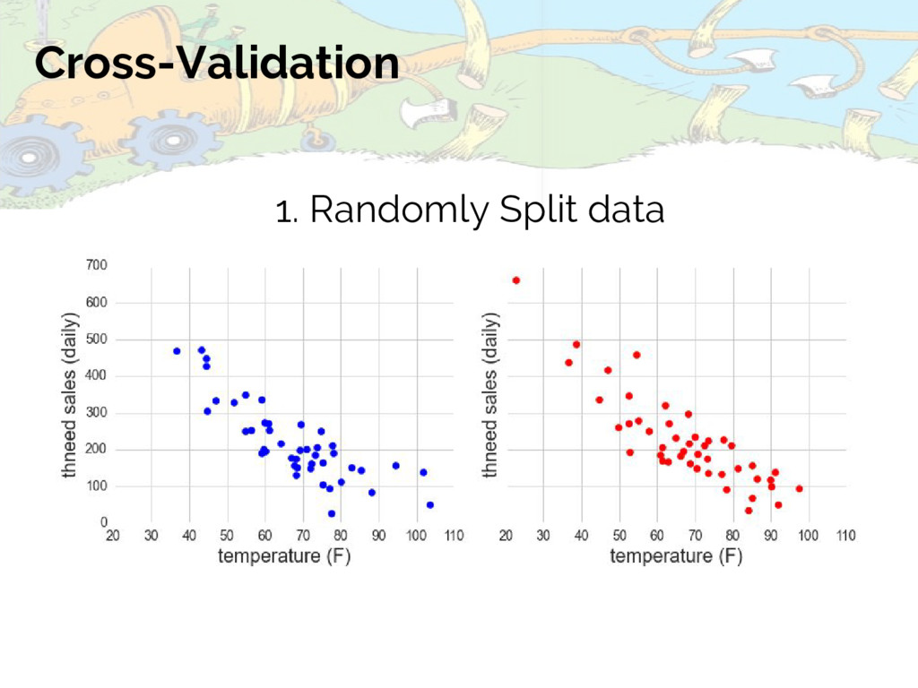
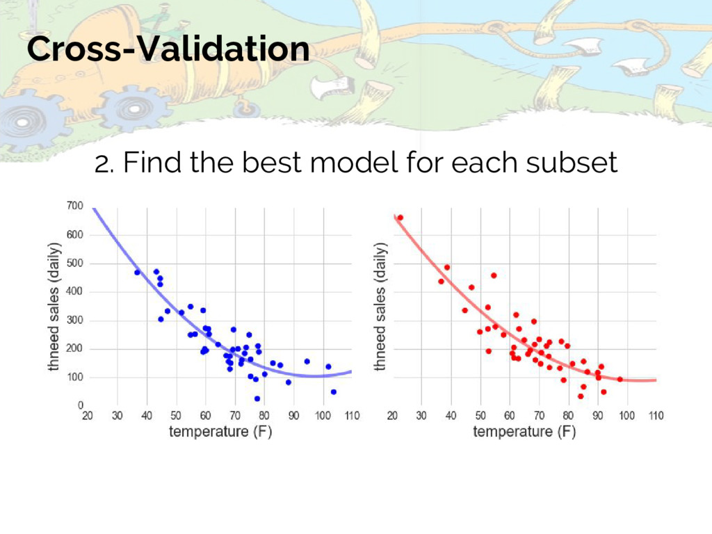
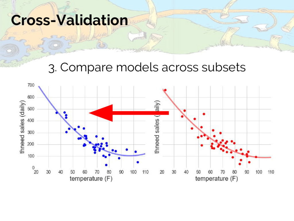
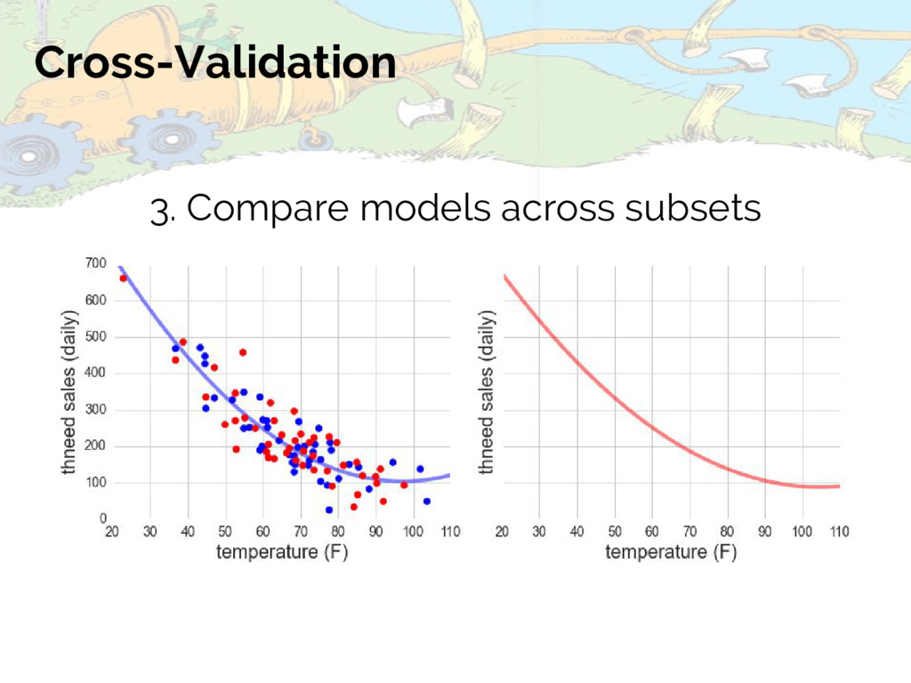
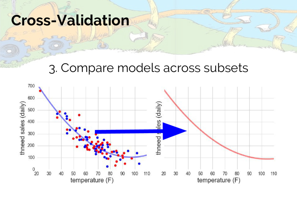
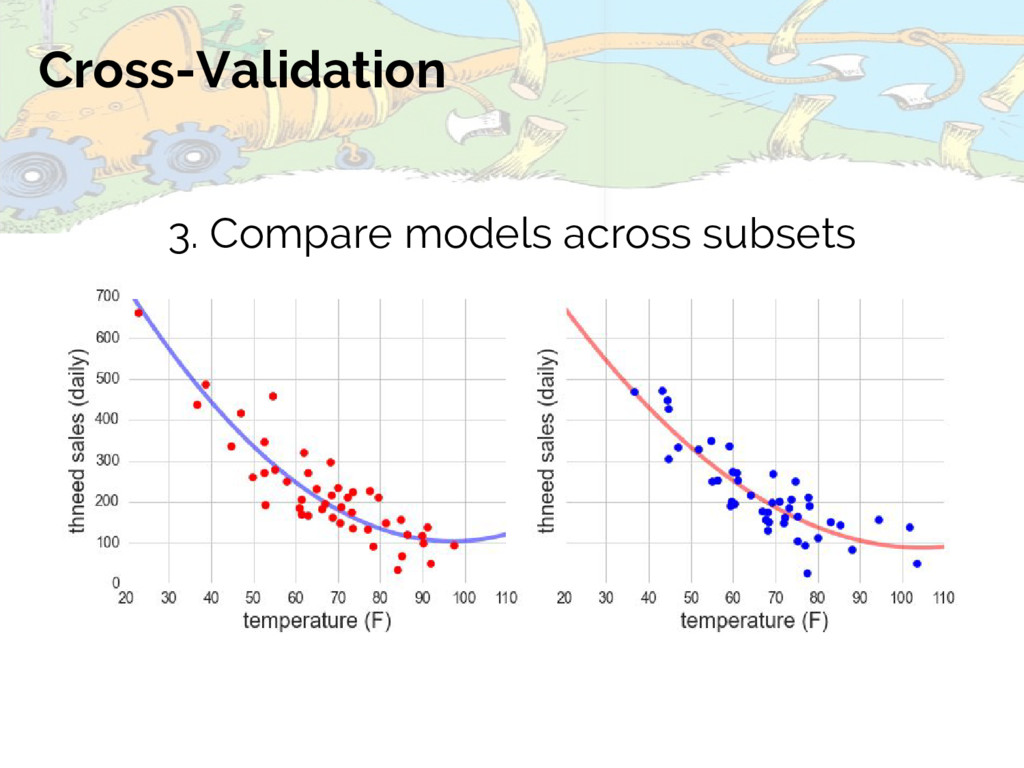
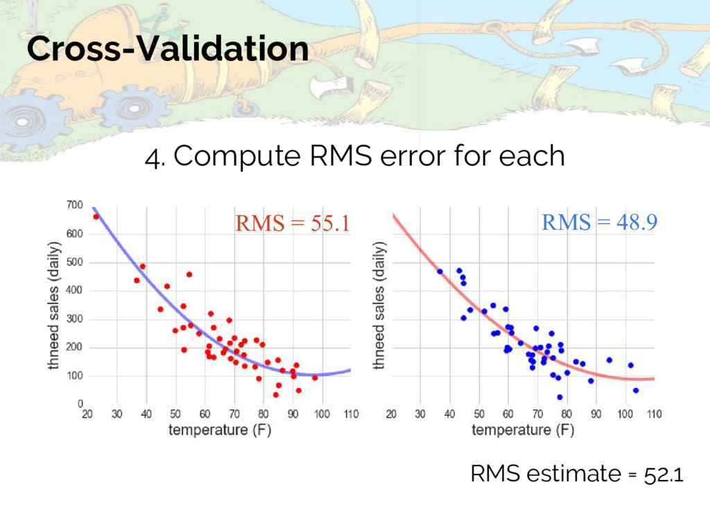
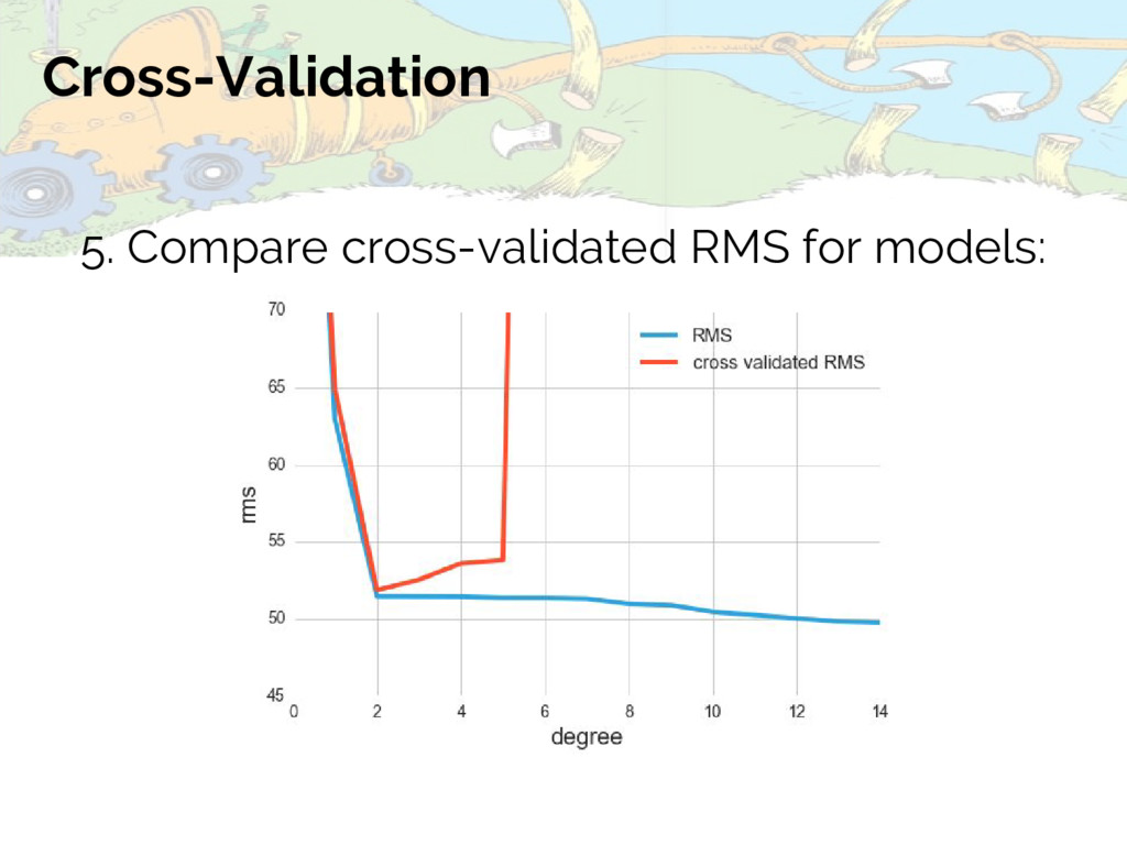
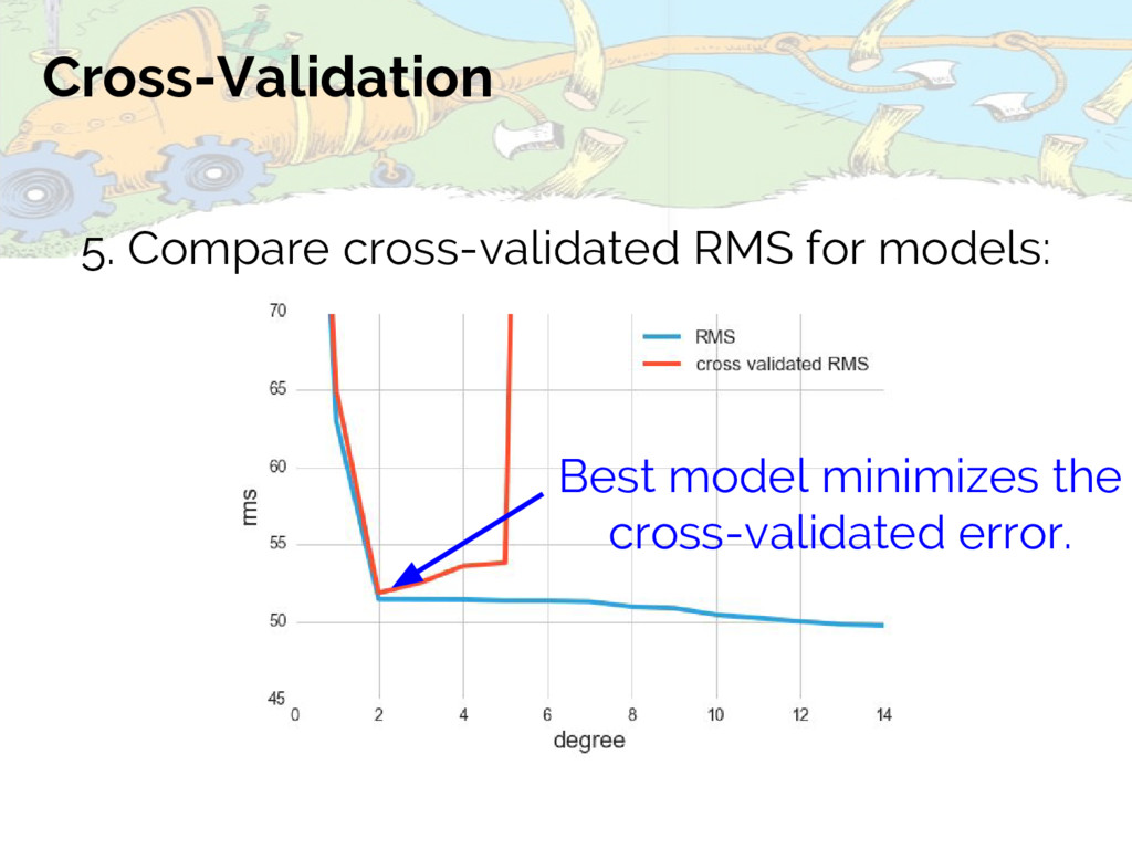
133. Notes on Cross-Validation: - This was “2-fold” cross-validation; other CV schemes exist & may perform better for your data (see e.g. scikit-learn docs) - Cross-validation is the go-to method for model evaluation in machine learning, as statistics of the models are often not known in the classical sense. - Again: caveats about selection bias and independence in data.
134. Four Recipes for Hacking Statistics: 1. Direct Simulation 2. Shuffling 3. Bootstrapping 4. Cross Validation
135. Sampling Methods allow you to use intuitive computational approaches in place of often non-intuitive statistical rules. If you can write a for-loop you can do statistical analysis.
136. Things I didn’t have time for: - Bayesian Methods: very intuitive & powerful approaches to more sophisticated modeling. (see e.g. Bayesian Methods for Hackers by Cam Davidson-Pilon) - Selection Bias: if you get data selection wrong, you’ll have a bad time. (See Chris Fonnesbeck’s Scipy 2015 talk, Statistical Thinking for Data Science) - Detailed considerations on use of sampling, shuffling, and bootstrapping. (I recommend Statistics Is Easy by Shasha & Wilson And Resampling: The New Statistics by Julian Simon)
137. – Dr. Seuss (attr)
138. ~ Thank You! ~ Email: jakevdp@uw.edu Twitter: @jakevdp Github: jakevdp Web: http://vanderplas.com/ Blog: http://jakevdp.github.io/ Slides available at http://speakerdeck.com/jakevdp/statistics-for-hackers/