An introduction to data-driven materials discovery

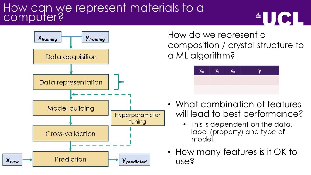
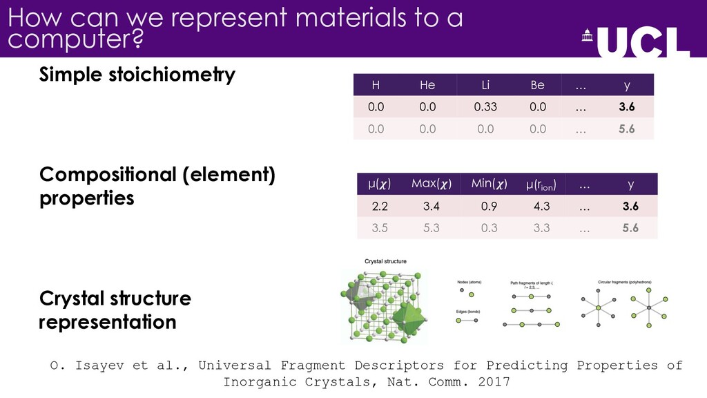
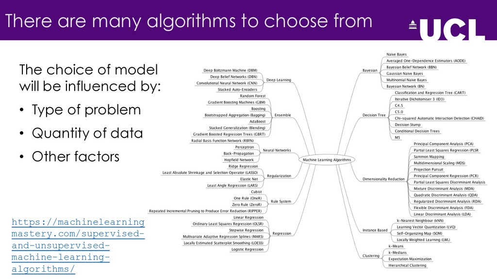
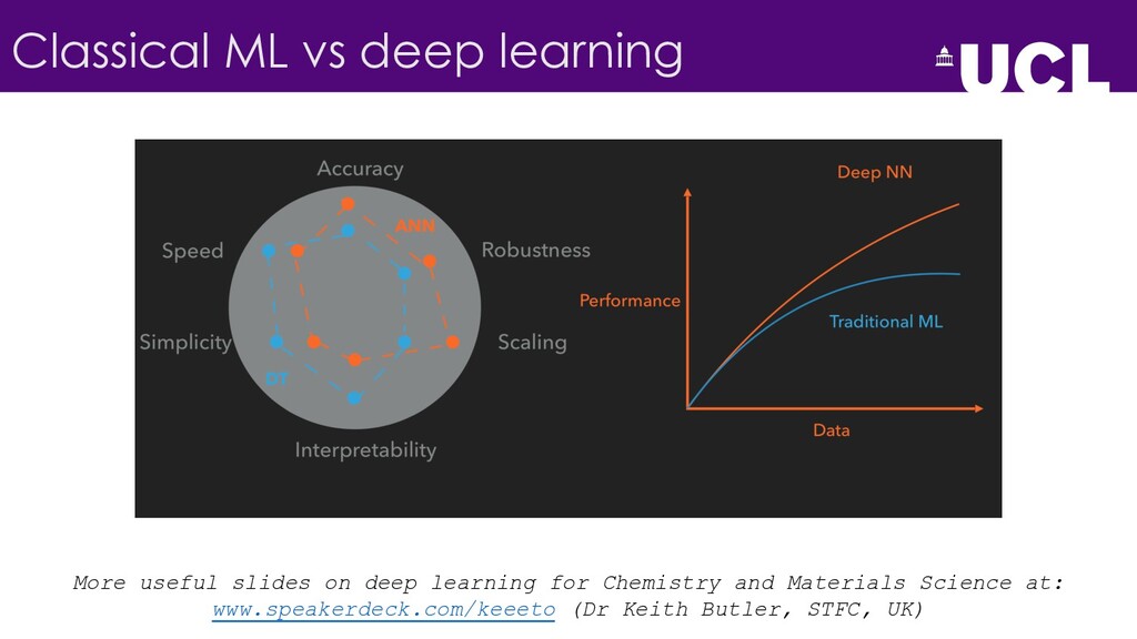
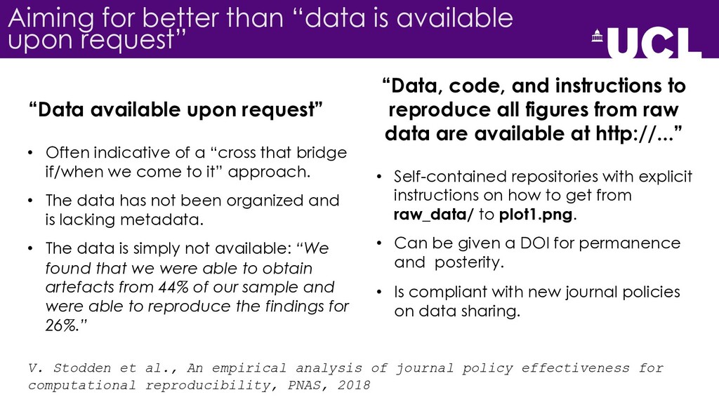
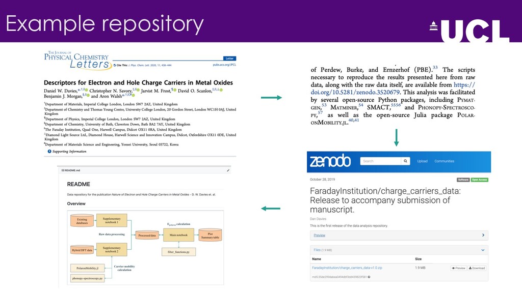
This tutorial-style presentation focuses on the use of data from first-principles calculations in materials discovery. It covers themes around materials databases, machine learning and open science. Links to practical tools and and references for further reading are provided.

Transcript

1. An introduction to data-driven materials discovery Dr Daniel Davies @danwdavies April, 2020 Department of Chemistry
2. Contents 1. The materials data landscape 2. Methods for solar energy materials discovery 3. Best practices for #OpenData and #OpenScience
3. Objectives 1. Become familiar with some useful databases of calculated materials properties and see how they are accessed. 2. Quantify to what extent the number of known materials represents the search space for new inorganic compounds. 3. Go through machine learning basics and take a look at a typical workflow setup. 4. Discuss the implications of data-driven science for reproducibility and open science. … And provide you with as many references as possible for further reading and practical tools.
4. 1. The materials data landscape
5. Data: The “4th paradigm” of science • “Big data” generated by experiments and computations has afforded unprecedented opportunities for data- driven techniques in materials science. • This has opened up new avenues for accelerated materials discovery. A. Agrawal and A. Choudhary, Perspective: Materials informatics and big data: realization of the fourth paradigm of science in Materials Science, APL Mater., 2016
6. Computing power in the 21st century “At a quintillion (1018) calculations each second, exascale supercomputers will more realistically simulate the processes involved in precision medicine, regional climate, additive manufacturing, the conversion of plants to biofuels, the relationship between energy and water use, the unseen physics in materials discovery and design, the fundamental forces of the universe, and much more.” https://www.top500.org/lists/2019/11/ https://exascaleproject.org/
7. Density functional theory (DFT) First-principles materials modelling: • Use Schrödinger equation and chemical composition as sole input • Simulate properties of materials • Accurate, unbiased, predictive F. Bechstedt, Many-body approach to electronic excitations, 2015 Hohenberg-Kohn (1964) Kohn-Sham (1965) Schrödinger (1887) Dirac (1902) Thomas-Fermi Density Functional Dynamic Mean Field
8. Data from DFT
9. The Materials Project http://materialsproject.org
10. AFLOW http://aflowlib.org/
11. NoMaD https://nomad-repository.eu/
12. Databases in materials science https://github.com/tilde-lab/awesome- materials-informatics J. Hill et al., Materials Science with large- scale data and informatics: Unlocking new opportunities, MRS Bull., 2016
13. Database access Access Pros Cons Web browser No knowledge of database software required Data can only be presented/downloaded for one material at a time Data dump All data is downloaded as one file Database software often needed, data is not up-to- date API Can query up-to-date data with advanced queries Programming knowledge required
14. API Example criteria = { ‘formula’: {‘$contains’: [‘Fe’]}, ‘band_gap’: {‘$gt’: 0.8} } properties = [‘structure’, ‘e_above_hull’, ‘spacegroup’] result = query(criteria, properties)
15. The search space for new materials • We have looked at databases containing calculated properties of existing materials, and will come back to how they can be leveraged in the search for new materials shortly. • We might first ask the question: “how much can there be left to discover?”
16. hydrogen 1 H 1.00794 lithium 3 Li 6.941 beryllium 4 Be 9.01218 sodium 11 Na 22.9898 magnesium 12 Mg 24.3050 potassium 19 K 39.0983 calcium 20 Ca 40.078 rubidium 37 Rb 85.4678 strontium 38 Sr 87.62 cesium 55 Cs 132.9055 barium 56 Ba 137.327 scandium 21 Sc 44.9559 titanium 22 Ti 47.867 vanadium 23 V 50.9415 chromium 24 Cr 51.9961 manganese 25 Mn 54.938 iron 26 Fe 55.845 cobalt 27 Co 58.9331 nickel 28 Ni 58.6934 copper 29 Cu 63.546 zinc 30 Zn 65.38 galium 31 Ga 69.723 germanium 32 Ge 72.64 aluminium 13 Al 26.9815 silicon 14 Si 28.0855 boron 5 B 10.811 carbon 6 C 12.0107 nitrogen 7 N 14.0067 oxygen 8 O 15.9994 phosphorus 15 P 30.9737 sulfur 16 S 32.065 arsenic 33 As 74.9216 selenium 34 Se 78.96 fluorine 9 F 18.9984 neon 10 Ne 20.1797 chlorine 17 Cl 35.453 argon 18 Ar 39.948 bromine 35 Br 79.904 krypton 36 Kr 83.798 thallium 81 Tl 204.3833 lead 82 Pb 207.2 indium 49 In 114.818 tin 50 Sn 118.710 antimony 51 Sb 121.760 tellurium 52 Te 127.60 bismuth 83 Bi 208.980 polonium 84 Po 209 iodine 53 I 126.904 xenon 54 Xe 131.293 astatine 85 At 210 radon 86 Rn 222 yttrium 39 Y 88.9059 zirconium 40 Zr 91.224 niobium 41 Nb 92.906 molybdenum 42 Mo 95.96 technetium 43 Tc 98 ruthenium 44 Ru 101.07 rhodium 45 Rh 102.9055 palladium 46 Pd 106.42 silver 47 Ag 107.8682 cadmium 48 Cd 112.411 hafnium 72 Hf 178.49 tantalum 73 Ta 180.9478 tungsten 74 W 183.84 rhenium 75 Re 186.207 osmium 76 Os 190.23 iridium 77 Ir 192.217 platinum 78 Pt 195.084 gold 79 Au 196.9666 mercury 80 Hg 200.59 helium 2 He 4.00260 Walsh Materials Design SMACT Periodic Table lanthanides actinides and other hard-to- pronounce elements +1,-1 +1 +1 +1 +1 +1 +2 +2 +2 +2 +2 +3 +3,+4 tt  +2,+3,+6 +2,+4,+7 +2,+3,+6 +2,+3 +2 +1,+2 +2 +3 tttttt  -3,+3,+5 -2 -1 +3 -4,+4 -3,+3,+5 -2,+2,+4 +6 -1,+1,+3 +5 +7 -1  t  +5,+7 +3 -4,+2,+4 -3,+3,+5 -2,+2,+4 +6 -1,+1,+3 +5 +7 +3 +4 +3,+5 +4,+6 +4,+7 t  +2,+3 +2,+4 +1 +2 +3 -4,+2,+4 -3,+3,+5 -2,+2,+4 +6 +4 +3,+5 t  +4,+6,+7 +4,+8 +3,+4 t  +1,+3 +1,+2 +1,+3 +2,+4 +3,+5 -2,+2,+4 -1,+1 tin 50 Sn 118.710 -4,+2,+4 common oxidation states atomic mass elemental symbol atomic number elemental name +2,+6 +2,+4,+6 +2 103 elements = ~400 species (that include oxidation state) of interest Building blocks for new inorganic materials
17. Element combinations and heuristic limits r Aw Bx Aw Bx Cy Aw Bx Cy Dz nCr 81,003 107 109 With stoichi- ometry 106 109 1012 Counting combinations: n = 403 species Aw Bx Cy Dz w,x,y,z ≤ 8 1. Charge neutrality: wqA + xqB + yqC + zqD = 0 2. Electronegativity order: Cation < Anion Imposing chemical rules:
18. D. W. Davies et al., Computational screening of all stoichiometric inorganic materials, Chem, 2016 Element combinations and heuristic limits
19. SMACT: Tools for generating chemical search spaces http://smact.readthedocs.io
20. All of this enumeration represents a low- end estimate We have only considered: • Stoichiometrically precise compositions • Up to quaternary (n=4) • With a limited stoichiometry range (1 > w,x,y,z > 8) and have totally ignored: • Variations in crystal structure (polymorphism) • Site occupancy/disorder • Defects • ... Large areas of unexplored composition space and a good starting point Moving towards more realistic materials accelerates the combinatorial explosion
21. Section summary • Computing power + improved theory + improved software = lots of usable materials data. • Databases containing materials properties are growing in number, many can now be accessed programatically using API. • The search space for new inorganic materials is vast within strict limits, and infinite otherwise. • Tools to explore the inorganic search space: http://smact.readthedocs.io
22. 2. Methods for solar energy materials discovery
23. Computable properties for solar energy materials A. Ganose et al., Beyond methylammonium lead iodide: prospects for the emergent field of ns2 containing solar absorbers, Chem. Commun., 2016 • We can now accurately calculate a wide range of optoelectronic properties. • These require widely varying amounts of computing power.
24. Inspiration from early semiconductor prediction Goodman (1958) Chen (2009) Pamplin (1963) Ideas of about valence, charge, electronegativity and ionicity have been used to predict new semiconductor band gaps for decades. C. H. Goodman, The prediction of semiconducting properties in inorganic compounds, J. Phys. Chem. Sol., 1958 S. Chen et al., Electronic structure and stability of quaternary chalcogenide semiconductors derived from cation cross-substitution of II-VI and I-III-VI2 compounds, PRB, 2009
25. Heuristics for band energy prediction • Nethercot (1974): Extension of Mulliken electronegativity to get mid-gap energy • Harrison (1980): Band gap estimates from tabulated values of s- and p- state eigenvalues • Pelatt (2011): Solid state energy scale from binary semiconductor ionisation potentials and electron affinities for VBM and CBM estimates A. H. Nethercot, prediction of fermi energies and photoelectric threshold based on electronegativity concepts, Phys. Rev. Lett 1974 W. A. Harrison, Electronic structure and the properties of solids, 1980 B. D. Pelatt et al., Atomic solid state energy scale, JACS, 2011
26. Beyond heuristics: Machine learning (ML) in materials science Targeting discovery of new compounds Enhancing theoretical chemistry Assisting characterization Mining existing literature
27. ML defined The field of study that gives computers the ability to learn without being explicitly programmed. Computer science Data science AI ML Data mining Command Action Data Action Model Traditional ML
28. Origins of ML Historical mentions of ML in books (Google Ngram viewer, 2020) IBM Journal of Research and Development, 1959
29. Some categories of ML Technique Input is known Output is known Method Supervised learning Yes Yes Analyze combinations of known inputs and outputs to predict future outputs based on new inputs Unsupervised learning Yes No Analyze inputs to generate outputs Reinforcement learning No Yes Keep trying input variables to reach a desired output (goal)
30. From linear regression to supervised machine learning x y Label Weights Feature • Linear regression works by finding a line that gives the best fit to the data. • Linear regression works by finding the weights that lead to the lowest cost. • Cost is almost always the “loss” (error) i.e. how “off” the model is from the actual data. Cost (loss)
31. From linear regression to supervised machine learning x y Continuous Univariate regression x0 xi xn y Discrete Classification x0 xi xn y Continuous Multivariate regression • Band gap • Energy • Effective mass • Crystal structure type • Is insulating • Is defect tolerant • Every 1st year undergrad experiment
32. Typical ML workflow Data acquisition Data representation Model building Cross-validation Prediction xtraining ytraining xnew ypredicted Supervised ML workflow: • Step 1: Model training and optimisation – getting from training data to the best possible built model. • Step 2: Prediction – Using the newly built model on unlabeled data. Hyperparameter tuning
33. Up to 90% of time can be spent selecting and scrubbing data Data acquisition Data representation Model building Cross-validation Prediction xtraining ytraining xnew ypredicted Probably the most (researcher) time is spent “data wrangling”- removing/replacing incomplete entries, transforming the data structure, dealing with outliers… Other key considerations: • Quality • Quantity • Utility • Reliability • Diversity Hyperparameter tuning
34. How can we represent materials to a computer? Data acquisition Data representation Model building Cross-validation Prediction xtraining ytraining xnew ypredicted Hyperparameter tuning How do we represent a composition / crystal structure to a ML algorithm? x0 xi xn y • What combination of features will lead to best performance? • This is dependent on the data, label (property) and type of model. • How many features is it OK to use?
35. How can we represent materials to a computer? Simple stoichiometry Compositional (element) properties Crystal structure representation µ() Max() Min() µ(rion ) … y 2.2 3.4 0.9 4.3 … 3.6 3.5 5.3 0.3 3.3 … 5.6 H He Li Be … y 0.0 0.0 0.33 0.0 … 3.6 0.0 0.0 0.0 0.0 … 5.6 O. Isayev et al., Universal Fragment Descriptors for Predicting Properties of Inorganic Crystals, Nat. Comm. 2017
36. There are many the models and loss functions to choose from Data acquisition Data representation Model building Cross-validation Prediction xtraining ytraining xnew ypredicted We have to choose: • Algorithm (model type) • Loss function • Model evaluation strategy Loss function: Metric to score model (how “off” from ground truth) Cross-validation: Systematically leave some data out to test model Hyperparameter tuning
37. There are many algorithms to choose from The choice of model will be influenced by: • Type of problem • Quantity of data • Other factors https://machinelearning mastery.com/supervised- and-unsupervised- machine-learning- algorithms/
38. There are many algorithms to choose from The choice of model will be influenced by: • Type of problem • Quantity of data • Other factors https://scikit-learn.org/stable/tutorial/machine_learning_map/
39. Classical ML vs deep learning More useful slides on deep learning for Chemistry and Materials Science at: www.speakerdeck.com/keeeto (Dr Keith Butler, STFC, UK)
40. There are many loss functions to choose from • Different loss functions respond differently to outliers, noise and under- vs over-prediction. • This, in turn, impacts on how “well” a given model is interpreted to be performing. • E.g. MAE more robust to outliers than MSE Distance from true value Penalty https://heartbeat.fritz.ai/5-regression-loss-functions-all-machine-learners- should-know-4fb140e9d4b0
41. Cross validation and hyperparameters Model building Cross-validation Hyperparameter tuning Adjust hyperparameters K. T. Butler et al., Machine learning for molecular and materials science, Nature 2018
42. Overfitting and underfitting Total prediction error is comprised of: • Bias: From oversimplified models that do not correctly capture underlying patterns in the data. • Variance: From complex models that do not generalize well beyond the training data. • Irreducible errors: That we can’t do anything about. High bias High variance These issues are hard to spot in higher dimensional space. Figure from www.speakerdeck.com/keeeto (Dr Keith Butler, STFC, UK)
43. Example workflow: Predicting band gap from composition Band gap of 35 ternary semiconductors RMSE = 0.66 eV Band gap of 800 oxides Solid State Energy (SSE, see Part 1) is a useful, cheap descriptor. But, not for oxides.
44. Example workflow: Predicting band gap from composition x: composition y: GLLB-sc band gap 800 oxides ML model New data Output Training data training prediction Predicted band gap 1.1M oxides x: composition Input data from Castelli et al., New Light-Harvesting Materials Using Accurate and Efficient Bandgap Calculations, Adv. Energy. Mat., 2015
45. Example workflow: Predicting band gap from composition Band gap of 800 oxides (10-fold cross validation) RMSE = 0.95 eV + Error + Number of trees
46. Example workflow: Predicting band gap from composition Distribution of GLLB-sc band gaps for 800 oxides Distribution of PBE band gap range for oxide compositions 8% D. W. Davies et al., Data-Driven Discovery of Photoactive Quaternary Oxides Using First-Principles Machine Learning, Chem. Mater., 2019
47. Further examples beyond compositional descriptors
48. Further reading
49. References and resources • A Critical Review of Machine Learning of Energy Materials: https://doi.org/10.1002/aenm.201903242 • Accelerating materials science with high-throughput computations and machine learning: https://doi.org/10.1016/j.commatsci.2019.01.013 • The Materials Simulation Toolkit for Machine learning (MAST-ML): An automated open source toolkit to accelerate data-driven materials research : https://doi.org/10.1016/j.commatsci.2020.109544 • https://pymatgen.org/ - Inorganic compounds in python • https://scikit-learn.org/ - Machine learning in python • https://hackingmaterials.lbl.gov/matminer/ - Representing materials for ML in python • https://pandas.pydata.org/ - Data handling in python • https://www.tensorflow.org/ - Neural networks • http://megnet.crystals.ai/ - Open source neural network tools • https://scikit-optimize.github.io/stable/ - hyperparameter tuning for scikit-learn
50. Section summary • Historically, many heuristics have been used for theoretical semiconductor discovery. • Nowadays, property prediction is one of many ways in which ML can accelerate materials discovery. • ML can quickly become another combinatorial problem: At every step of a workflow there are decisions to be made. • Could be automated? (See http://hackingmaterials.lbl.gov/automatminer/)
51. 3. Best practices for Open Data and Open Science
52. The move towards Open Science • In science, we are usually building on previous work. • We can often only access the final results of such work, at various levels of granularity. • Plots/Figures • Tables • Text descriptions • It is more efficient (for us and our funders) if data and code is available so that work can be reproduced and/or reused. Open science: “Scholarly research that is collaborative, transparent and reproducible and whose outputs are publicly available.” EU report on open science policy platform recommendations, 2015
53. Key Open Science vocab • Rerun: Same people, modify setup • Repeat: Same people, same setup • Replicate: Different people, same setup • Reproduce: Different people, different setup • Reuse: Similar setup, different experiment See Dr Adam Jackson’s slides on open software: https://github.com/ajjackson/open- research-software Improve quality of research Improve efficiency of research
54. The burden of proof is higher for computational and data-driven studies • All scientific publications: • Announce a result. • Convince the reader that the result is correct. • Experimental papers should: • Describe the result. • Provide clear protocol for the result to be reproduced and built upon. • Computational paper should: • Provide the complete software development environment, data and set of instructions which generated the figures/tables. See Carole Goble’s slides on reproducibility: https://www.slideshare.net/carolegoble/what-is-reproducibility-gobleclean
55. Aiming for better than “data is available upon request” “Data available upon request” V. Stodden et al., An empirical analysis of journal policy effectiveness for computational reproducibility, PNAS, 2018 “Data, code, and instructions to reproduce all figures from raw data are available at http://...” • Often indicative of a “cross that bridge if/when we come to it” approach. • The data has not been organized and is lacking metadata. • The data is simply not available: “We found that we were able to obtain artefacts from 44% of our sample and were able to reproduce the findings for 26%.” • Self-contained repositories with explicit instructions on how to get from raw_data/ to plot1.png. • Can be given a DOI for permanence and posterity. • Is compliant with new journal policies on data sharing.
56. Example repository
57. Section summary • Avoid proprietary software/code and data formats • Use a license for your code and data: (https://choosealicense.com/) • Include raw data and metadata (as well as processed data) • Automate everything as far as possible • Make your data: • Findable • Available • Interoperable • Reusable
58. Thanks! @danwdavies