Cloud2Curve: Generation and Vectorization of Parametric Sketches

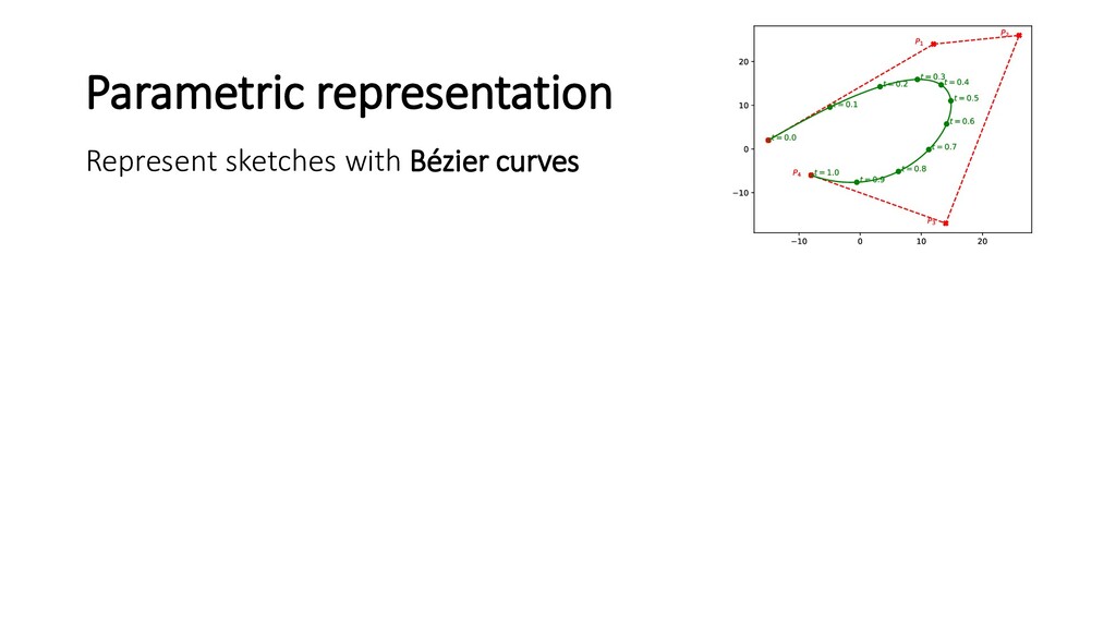
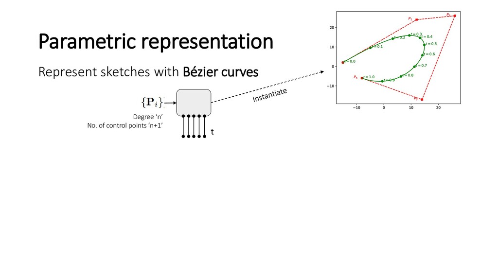
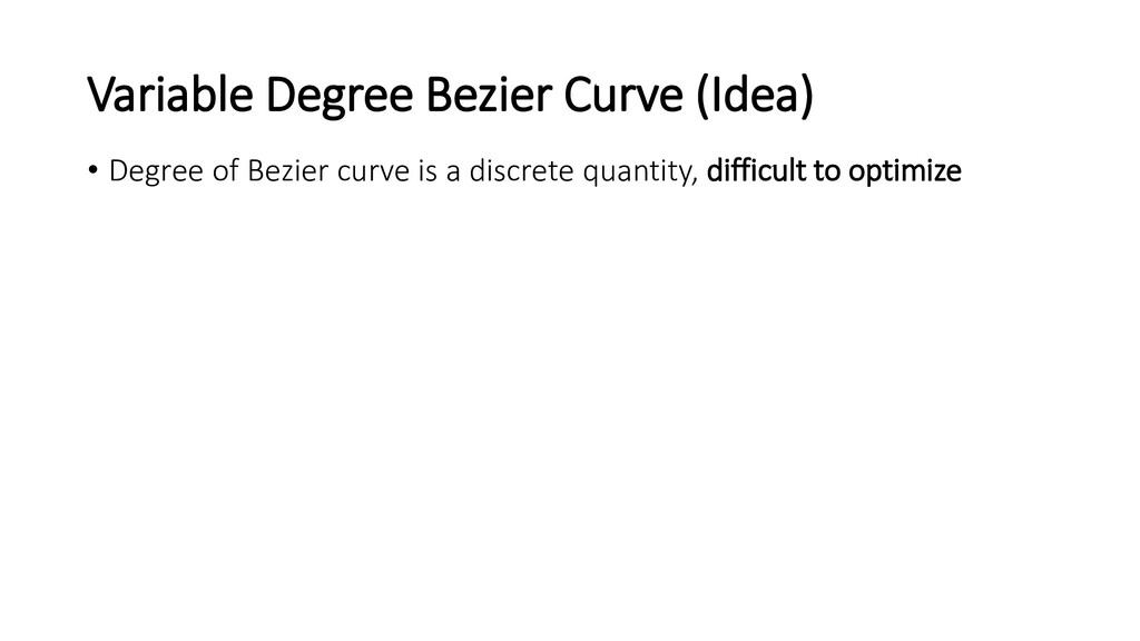
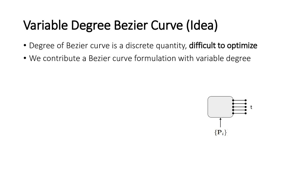
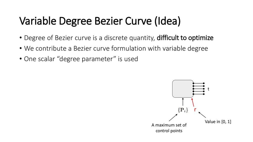
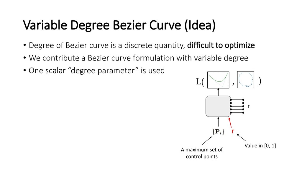
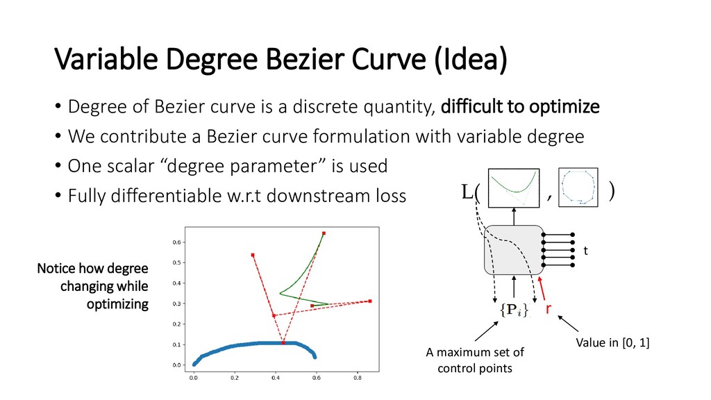
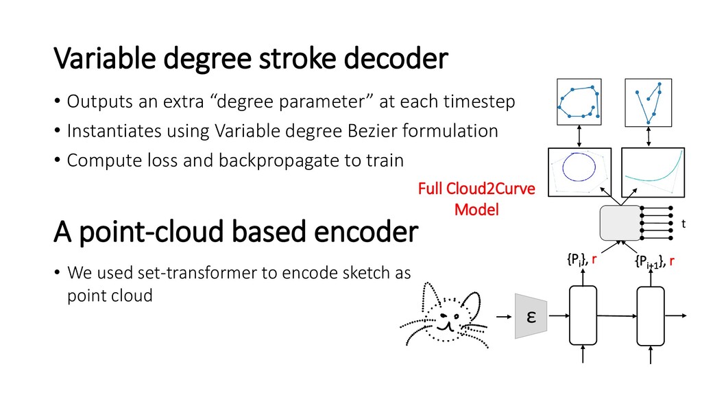
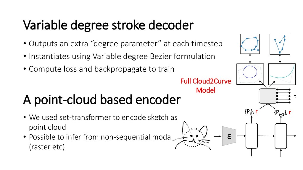
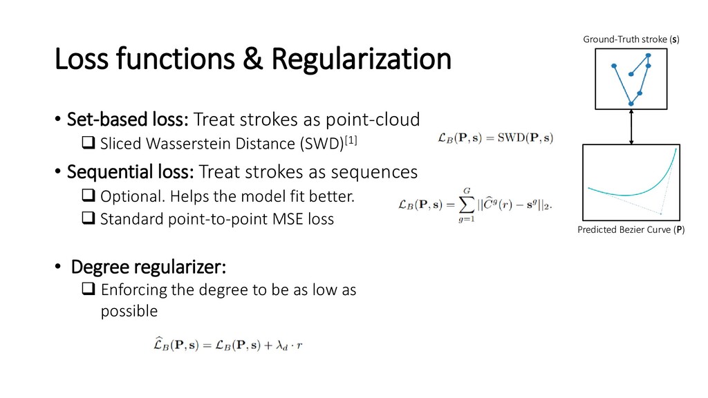
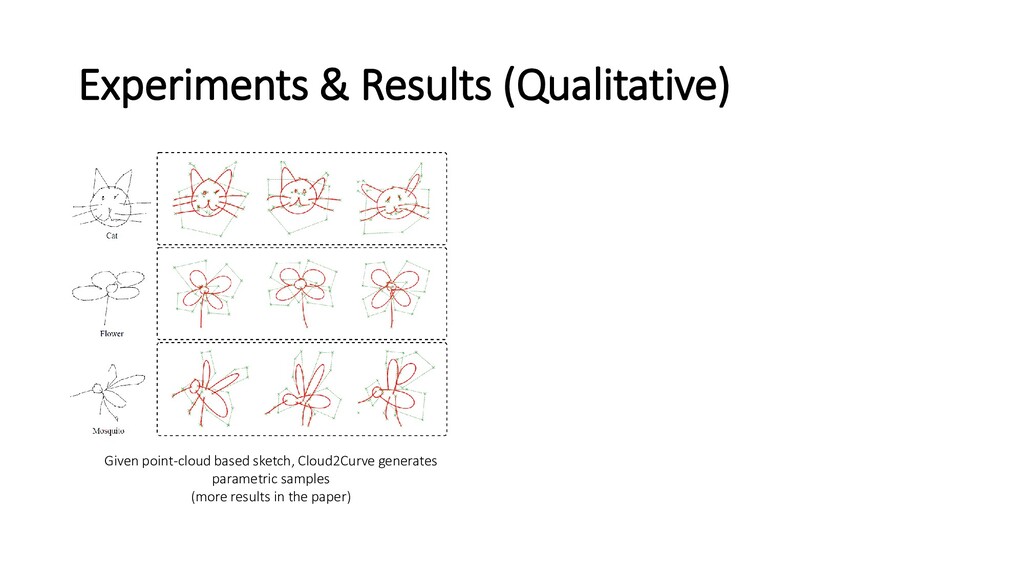
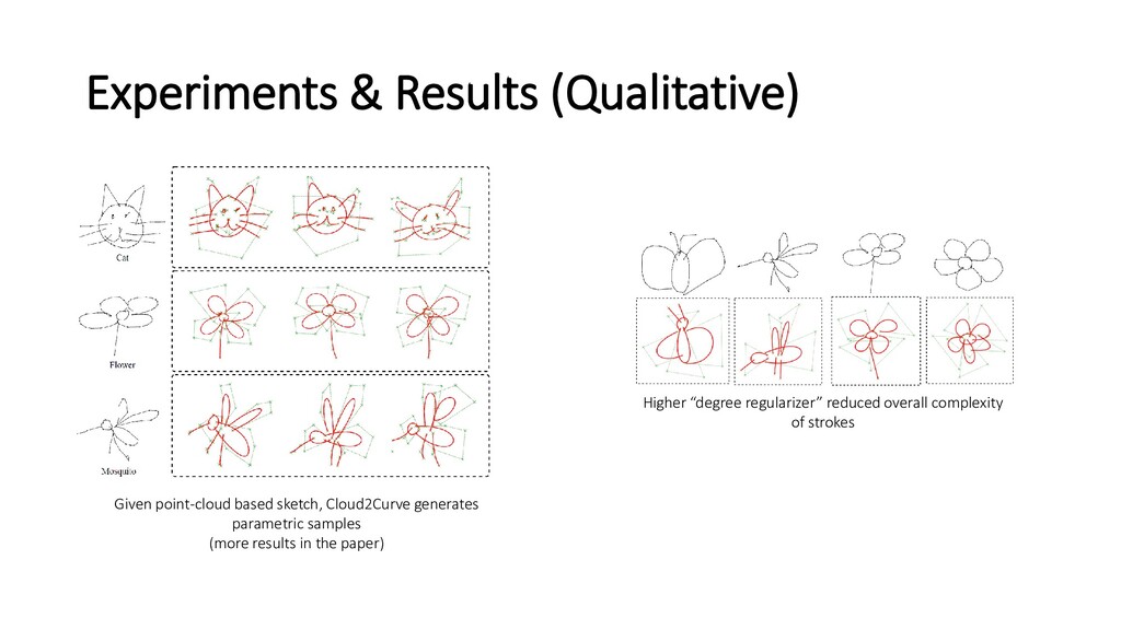
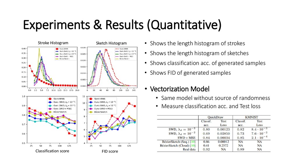
Analysis of human sketches in deep learning has advanced immensely through the use of waypoint-sequences rather than raster-graphic representations. We further aim to model sketches as a sequence of low-dimensional parametric curves. To this end, we propose an inverse graphics framework capable of approximating a raster or waypoint based stroke encoded as a point-cloud with a variable-degree Bezier curve. Building on this module, we present Cloud2Curve, a generative model for scalable high-resolution vector sketches that can be trained end-to-end using point-cloud data alone. As a consequence, our model is also capable of deterministic vectorization which
can map novel raster or waypoint based sketches to their corresponding high-resolution scalable Bezier equivalent. We evaluate the generation and vectorization capabilities of our model on Quick, Draw! and K-MNIST datasets.

Transcript

2. Cloud2Curve: Generation and Vectorization of Parametric Sketches Ayan Das1,2, Yongxin Yang1,2, Timothy Hospedales1,3, Tao Xiang1,2 and Yi-Zhe Song1,2 1 SketchX, CVSSP, University of Surrey, United Kingdom 2 iFlyTek-Surrey Joint Research Centre on Artificial Intelligence 3 University of Edinburgh, United Kingdom CVPR 2021 (Poster)
3. Traditional Sketch generation models • The state-of-the-art “SketchRNN”[1] [1] Ha, D., Eck, D.: A neural representation of sketch drawings. In: ICLR (2018) [2] Graves, A.: Generating Sequences With Recurrent Neural Networks. (2013)
4. Traditional Sketch generation models • The state-of-the-art “SketchRNN”[1] ❑ Uses Polyline representation [1] Ha, D., Eck, D.: A neural representation of sketch drawings. In: ICLR (2018) [2] Graves, A.: Generating Sequences With Recurrent Neural Networks. (2013)
5. Traditional Sketch generation models • The state-of-the-art “SketchRNN”[1] ❑ Uses Polyline representation ❑ Autoregressive generation of points[2] [1] Ha, D., Eck, D.: A neural representation of sketch drawings. In: ICLR (2018) [2] Graves, A.: Generating Sequences With Recurrent Neural Networks. (2013)
6. Traditional Sketch generation models • The state-of-the-art “SketchRNN”[1] ❑ Uses Polyline representation ❑ Autoregressive generation of points[2] … [1] Ha, D., Eck, D.: A neural representation of sketch drawings. In: ICLR (2018) [2] Graves, A.: Generating Sequences With Recurrent Neural Networks. (2013)
7. Traditional Sketch generation models • The state-of-the-art “SketchRNN”[1] ❑ Uses Polyline representation ❑ Autoregressive generation of points[2] Δp1 [0,0] Δpi Δpi-1 … [0,0] p1 p2 [1] Ha, D., Eck, D.: A neural representation of sketch drawings. In: ICLR (2018) [2] Graves, A.: Generating Sequences With Recurrent Neural Networks. (2013)
8. Traditional Sketch generation models • The state-of-the-art “SketchRNN”[1] ❑ Uses Polyline representation ❑ Autoregressive generation of points[2] Δp1 [0,0] Δpi Δpi-1 … [0,0] p1 p2 [1] Ha, D., Eck, D.: A neural representation of sketch drawings. In: ICLR (2018) [2] Graves, A.: Generating Sequences With Recurrent Neural Networks. (2013)
9. Traditional Sketch generation models • The state-of-the-art “SketchRNN”[1] ❑ Uses Polyline representation ❑ Autoregressive generation of points[2] Δp1 [0,0] Δpi Δpi-1 … [0,0] p1 p2 [1] Ha, D., Eck, D.: A neural representation of sketch drawings. In: ICLR (2018) [2] Graves, A.: Generating Sequences With Recurrent Neural Networks. (2013) [0,0] p1 p2 ~ ε Require polyline format for inference
10. Parametric representation
11. Parametric representation Represent sketches with Bézier curves
12. Parametric representation Represent sketches with Bézier curves Degree ‘n’ No. of control points ‘n+1’
13. Parametric representation Represent sketches with Bézier curves t Degree ‘n’ No. of control points ‘n+1’
14. Parametric representation Represent sketches with Bézier curves • Shorter in length • Arbitrary resolution • Scalable, High quality t Degree ‘n’ No. of control points ‘n+1’
15. Parametric representation Represent sketches with Bézier curves • Shorter in length • Arbitrary resolution • Scalable, High quality t Degree ‘n’ No. of control points ‘n+1’
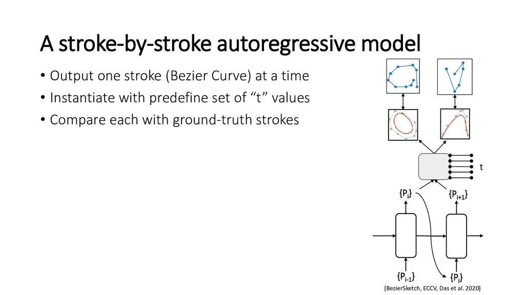
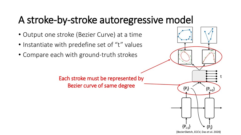
16. A stroke-by-stroke autoregressive model [BezierSketch, ECCV, Das et al. 2020]
17. A stroke-by-stroke autoregressive model {Pi } {Pi-1 } {Pi } {Pi+1 } • Output one stroke (Bezier Curve) at a time [BezierSketch, ECCV, Das et al. 2020]
18. A stroke-by-stroke autoregressive model {Pi } {Pi-1 } {Pi } {Pi+1 } • Output one stroke (Bezier Curve) at a time • Instantiate with predefine set of “t” values t [BezierSketch, ECCV, Das et al. 2020]
19. A stroke-by-stroke autoregressive model {Pi } {Pi-1 } {Pi } {Pi+1 } • Output one stroke (Bezier Curve) at a time • Instantiate with predefine set of “t” values • Compare each with ground-truth strokes t [BezierSketch, ECCV, Das et al. 2020]
20. A stroke-by-stroke autoregressive model {Pi } {Pi-1 } {Pi } {Pi+1 } • Output one stroke (Bezier Curve) at a time • Instantiate with predefine set of “t” values • Compare each with ground-truth strokes t Each stroke must be represented by Bezier curve of same degree [BezierSketch, ECCV, Das et al. 2020]
21. Variable Degree Bezier Curve (Idea)
22. Variable Degree Bezier Curve (Idea) • Degree of Bezier curve is a discrete quantity, difficult to optimize
23. Variable Degree Bezier Curve (Idea) • Degree of Bezier curve is a discrete quantity, difficult to optimize • We contribute a Bezier curve formulation with variable degree t
24. Variable Degree Bezier Curve (Idea) • Degree of Bezier curve is a discrete quantity, difficult to optimize • We contribute a Bezier curve formulation with variable degree • One scalar “degree parameter” is used t r A maximum set of control points Value in [0, 1]
25. Variable Degree Bezier Curve (Idea) • Degree of Bezier curve is a discrete quantity, difficult to optimize • We contribute a Bezier curve formulation with variable degree • One scalar “degree parameter” is used t r A maximum set of control points Value in [0, 1]
26. Variable Degree Bezier Curve (Idea) • Degree of Bezier curve is a discrete quantity, difficult to optimize • We contribute a Bezier curve formulation with variable degree • One scalar “degree parameter” is used t r L( , ) A maximum set of control points Value in [0, 1]
27. Variable Degree Bezier Curve (Idea) • Degree of Bezier curve is a discrete quantity, difficult to optimize • We contribute a Bezier curve formulation with variable degree • One scalar “degree parameter” is used • Fully differentiable w.r.t downstream loss t r L( , ) A maximum set of control points Value in [0, 1]
28. Variable Degree Bezier Curve (Idea) • Degree of Bezier curve is a discrete quantity, difficult to optimize • We contribute a Bezier curve formulation with variable degree • One scalar “degree parameter” is used • Fully differentiable w.r.t downstream loss t r L( , ) A maximum set of control points Notice how degree changing while optimizing Value in [0, 1]
29. Variable Degree Bezier Curve (Formulation)
30. Variable Degree Bezier Curve (Formulation) • The Bezier curve formula has three components (Time matrix, Degree matrix and Control Points)
31. Variable Degree Bezier Curve (Formulation) • The Bezier curve formula has three components (Time matrix, Degree matrix and Control Points) • Compute “Degree selector” R(r) Refer to the paper for details
32. Variable Degree Bezier Curve (Formulation) • The Bezier curve formula has three components (Time matrix, Degree matrix and Control Points) • Compute “Degree selector” R(r) • Augmented each component Refer to the paper for details
33. Variable degree stroke decoder
34. Variable degree stroke decoder {Pi }, r {Pi+1 }, r • Outputs an extra “degree parameter” at each timestep
35. Variable degree stroke decoder {Pi }, r {Pi+1 }, r t • Outputs an extra “degree parameter” at each timestep • Instantiates using Variable degree Bezier formulation
36. Variable degree stroke decoder {Pi }, r {Pi+1 }, r t • Outputs an extra “degree parameter” at each timestep • Instantiates using Variable degree Bezier formulation • Compute loss and backpropagate to train
37. Variable degree stroke decoder {Pi }, r {Pi+1 }, r t • Outputs an extra “degree parameter” at each timestep • Instantiates using Variable degree Bezier formulation • Compute loss and backpropagate to train A point-cloud based encoder • We used set-transformer to encode sketch as point cloud ε Full Cloud2Curve Model
38. Variable degree stroke decoder {Pi }, r {Pi+1 }, r t • Outputs an extra “degree parameter” at each timestep • Instantiates using Variable degree Bezier formulation • Compute loss and backpropagate to train A point-cloud based encoder • We used set-transformer to encode sketch as point cloud • Possible to infer from non-sequential modalities (raster etc) ε Full Cloud2Curve Model
39. Loss functions & Regularization Predicted Bezier Curve (P) Ground-Truth stroke (s)
40. Loss functions & Regularization • Set-based loss: Treat strokes as point-cloud ❑ Sliced Wasserstein Distance (SWD)[1] Predicted Bezier Curve (P) Ground-Truth stroke (s)
41. Loss functions & Regularization • Set-based loss: Treat strokes as point-cloud ❑ Sliced Wasserstein Distance (SWD)[1] • Sequential loss: Treat strokes as sequences ❑ Optional. Helps the model fit better. ❑ Standard point-to-point MSE loss Predicted Bezier Curve (P) Ground-Truth stroke (s)
42. Loss functions & Regularization • Set-based loss: Treat strokes as point-cloud ❑ Sliced Wasserstein Distance (SWD)[1] • Sequential loss: Treat strokes as sequences ❑ Optional. Helps the model fit better. ❑ Standard point-to-point MSE loss Predicted Bezier Curve (P) Ground-Truth stroke (s) • Degree regularizer: ❑ Enforcing the degree to be as low as possible
43. Loss functions & Regularization • Set-based loss: Treat strokes as point-cloud ❑ Sliced Wasserstein Distance (SWD)[1] • Sequential loss: Treat strokes as sequences ❑ Optional. Helps the model fit better. ❑ Standard point-to-point MSE loss Predicted Bezier Curve (P) Ground-Truth stroke (s) • Degree regularizer: ❑ Enforcing the degree to be as low as possible High value of degree regularizer enforces same stroke to acquire less degree
44. Experiments & Results (Qualitative)
45. Experiments & Results (Qualitative) Given point-cloud based sketch, Cloud2Curve generates parametric samples (more results in the paper)
46. Experiments & Results (Qualitative) Given point-cloud based sketch, Cloud2Curve generates parametric samples (more results in the paper) Higher “degree regularizer” reduced overall complexity of strokes
47. Experiments & Results (Quantitative)
48. Experiments & Results (Quantitative) • Shows the length histogram of strokes • Shows the length histogram of sketches Stroke Histogram Sketch Histogram
49. Experiments & Results (Quantitative) • Shows the length histogram of strokes • Shows the length histogram of sketches • Shows classification acc. of generated samples • Shows FID of generated samples Stroke Histogram Sketch Histogram Classification score FID score
50. Experiments & Results (Quantitative) • Shows the length histogram of strokes • Shows the length histogram of sketches • Shows classification acc. of generated samples • Shows FID of generated samples • Vectorization Model • Same model without source of randomness • Measure classification acc. and Test loss Stroke Histogram Sketch Histogram Classification score FID score
51. Thank You Project page: https://ayandas.me/pubs/2021/03/01/pub-9.html