diffusion_talk_AD_PRISLAB.pdf

Talk given at BUPT. Elaborate tutorial on Diffusion Models

Transcript

1. Ayan Das PhD Student, University of Surrey DL Intern, MediaTek Research UK Diffusion Models Adv a ncements & Applic a tions Forward Di ff usion Reverse Di ff usion
2. Copyright (c) 2022 by Ayan Das (@ dasayan05) General Introduction
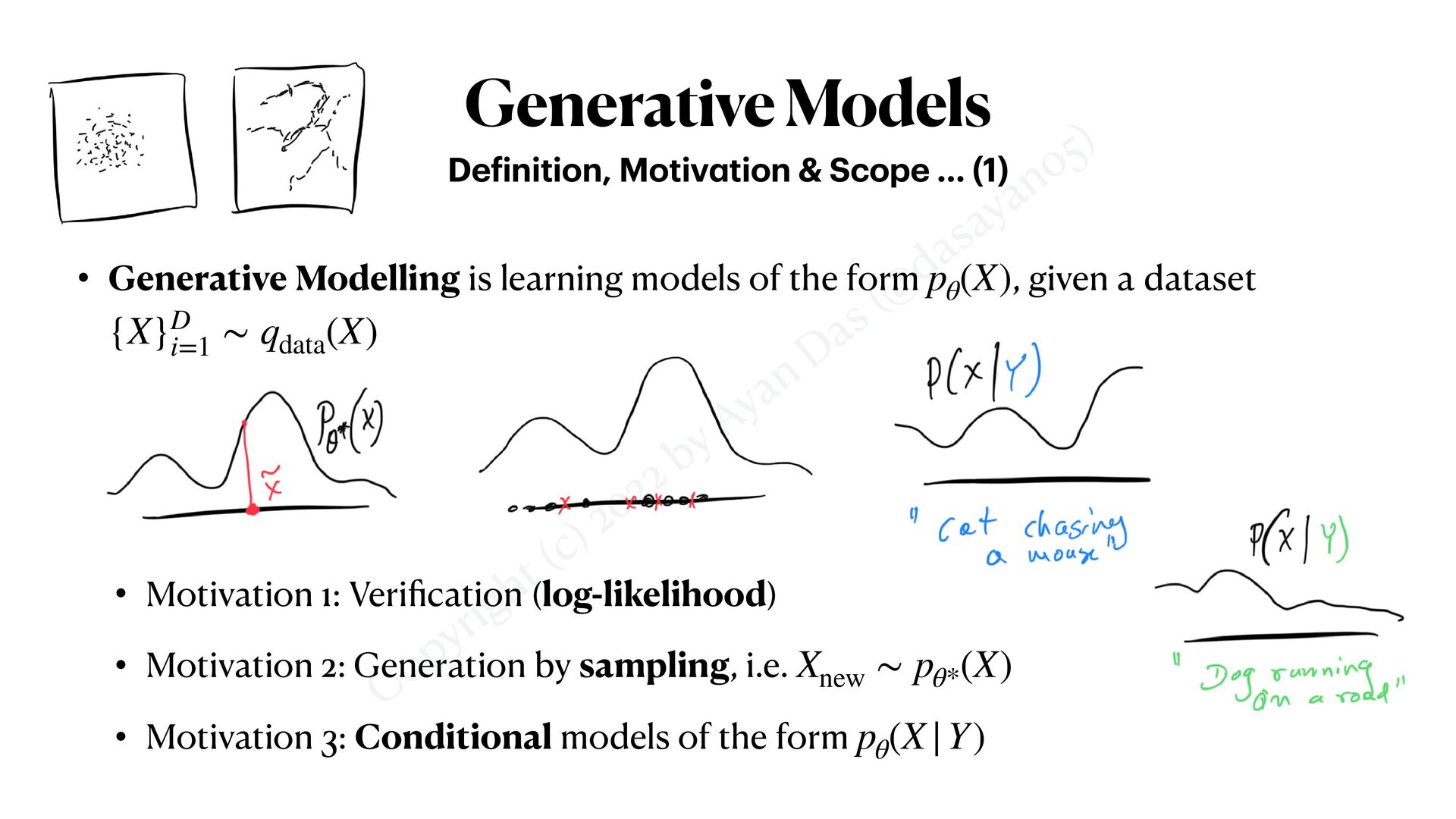
3. Copyright (c) 2022 by Ayan Das (@ dasayan05) Generative Models • Generative Modelling is learning models of the form , given a dataset pθ (X) {X}D i=1 ∼ qdata (X) De f inition, Motiv a tion & Scope … (1) • Motivation 1: Veri fi cation (log-likelihood) • Motivation 2: Generation by sampling, i.e. • Motivation 3: Conditional models of the form Xnew ∼ pθ* (X) pθ (X|Y)
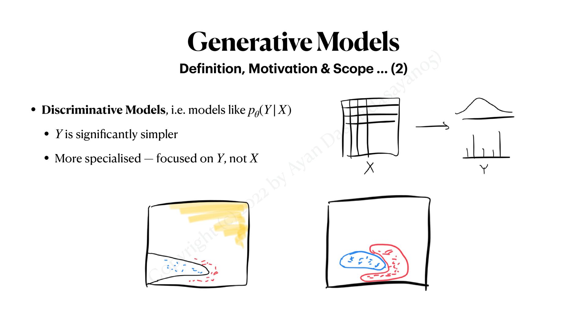
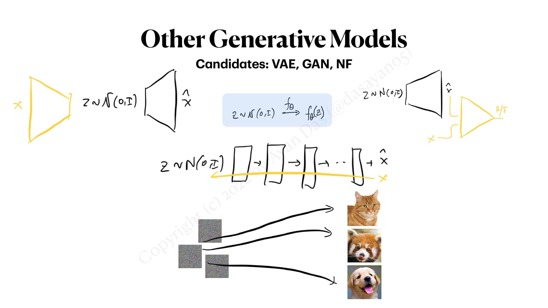
4. Copyright (c) 2022 by Ayan Das (@ dasayan05) Generative Models De f inition, Motiv a tion & Scope … (2) • Discriminative Models, i.e. models like • is signi fi cantly simpler • More specialised — focused on , not pθ (Y|X) Y Y X
5. Copyright (c) 2022 by Ayan Das (@ dasayan05) Diversity vs Fidelity The tr a de-off GANS VAEs
6. Copyright (c) 2022 by Ayan Das (@ dasayan05) Any model that can do both equally well ? .. or m a ybe control the tr a de-off
7. Copyright (c) 2022 by Ayan Das (@ dasayan05) Di ff usion Models
8. Copyright (c) 2022 by Ayan Das (@ dasayan05) Other Generative Models C a ndid a tes: VAE, GAN, NF
9. Copyright (c) 2022 by Ayan Das (@ dasayan05) Diffusion Models are different Wh a t m a kes it h a rd to work with ? Non-deterministic mapping
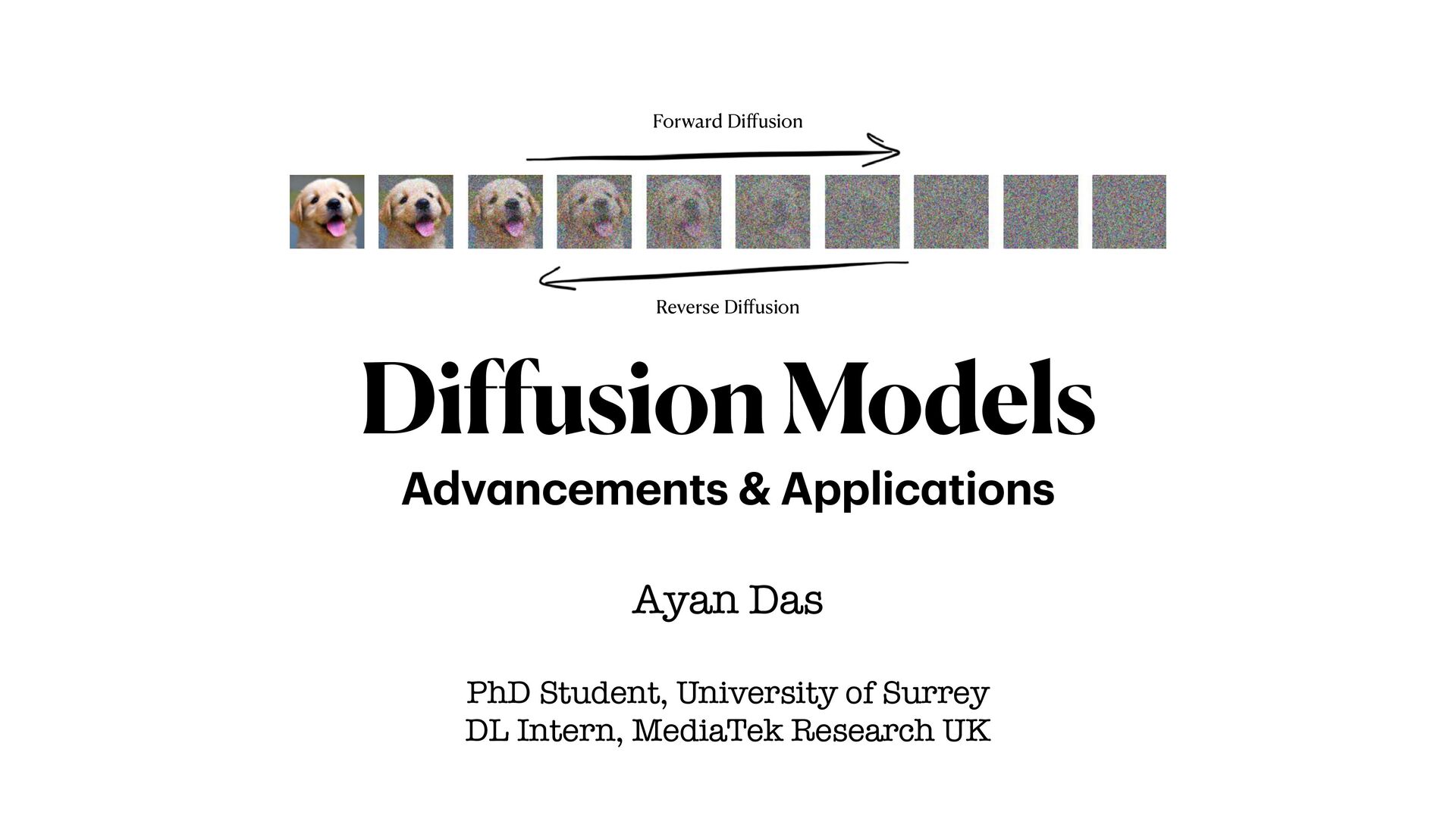
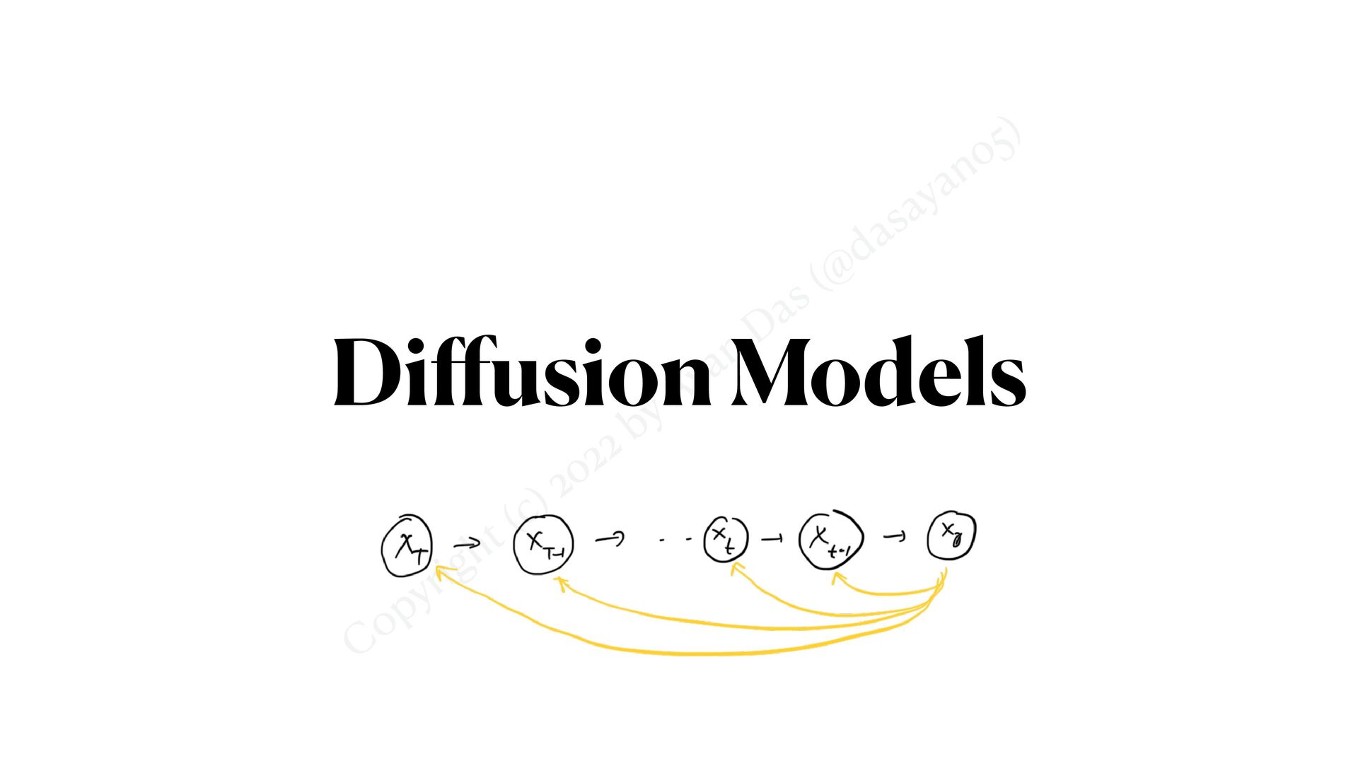
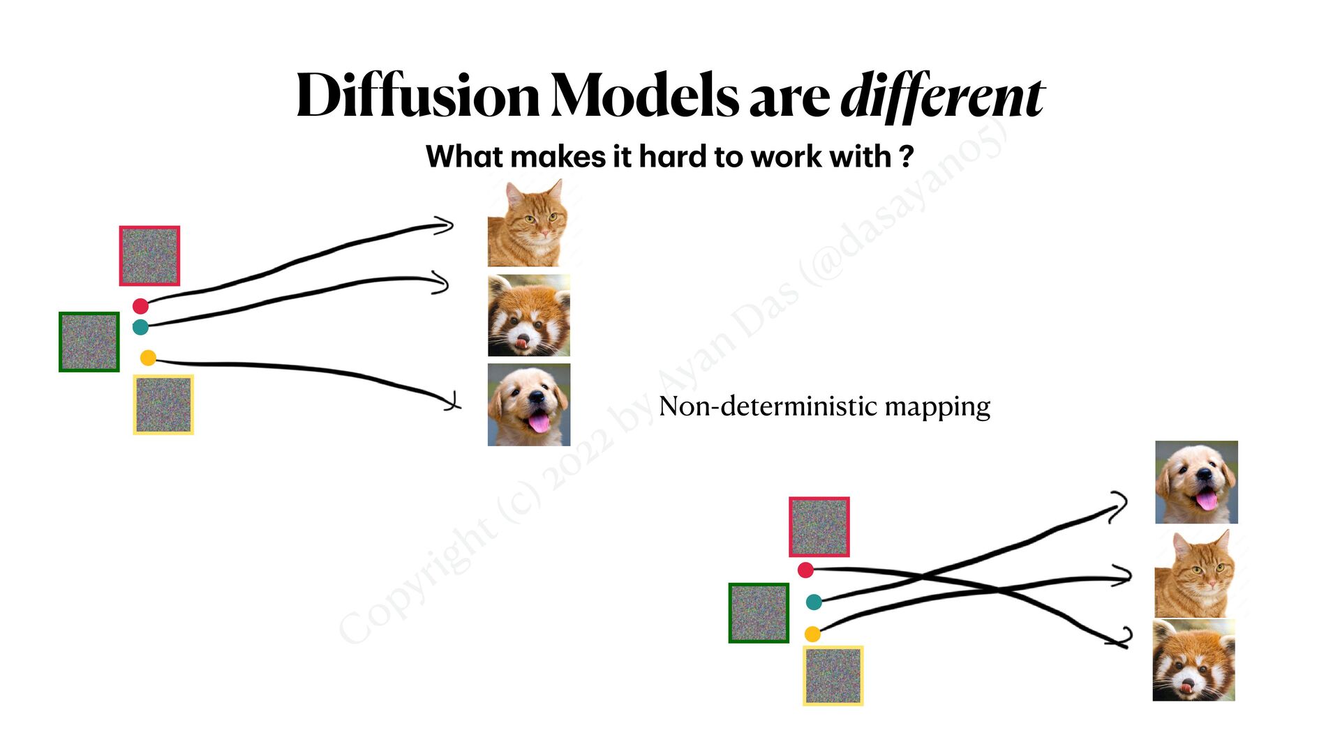
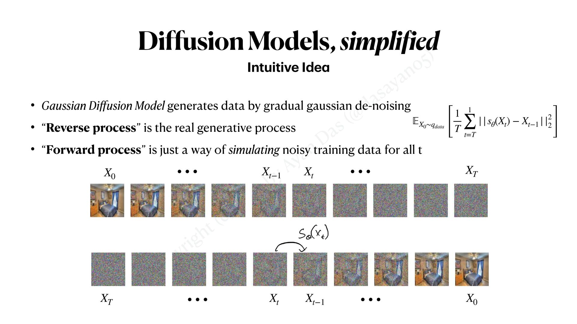
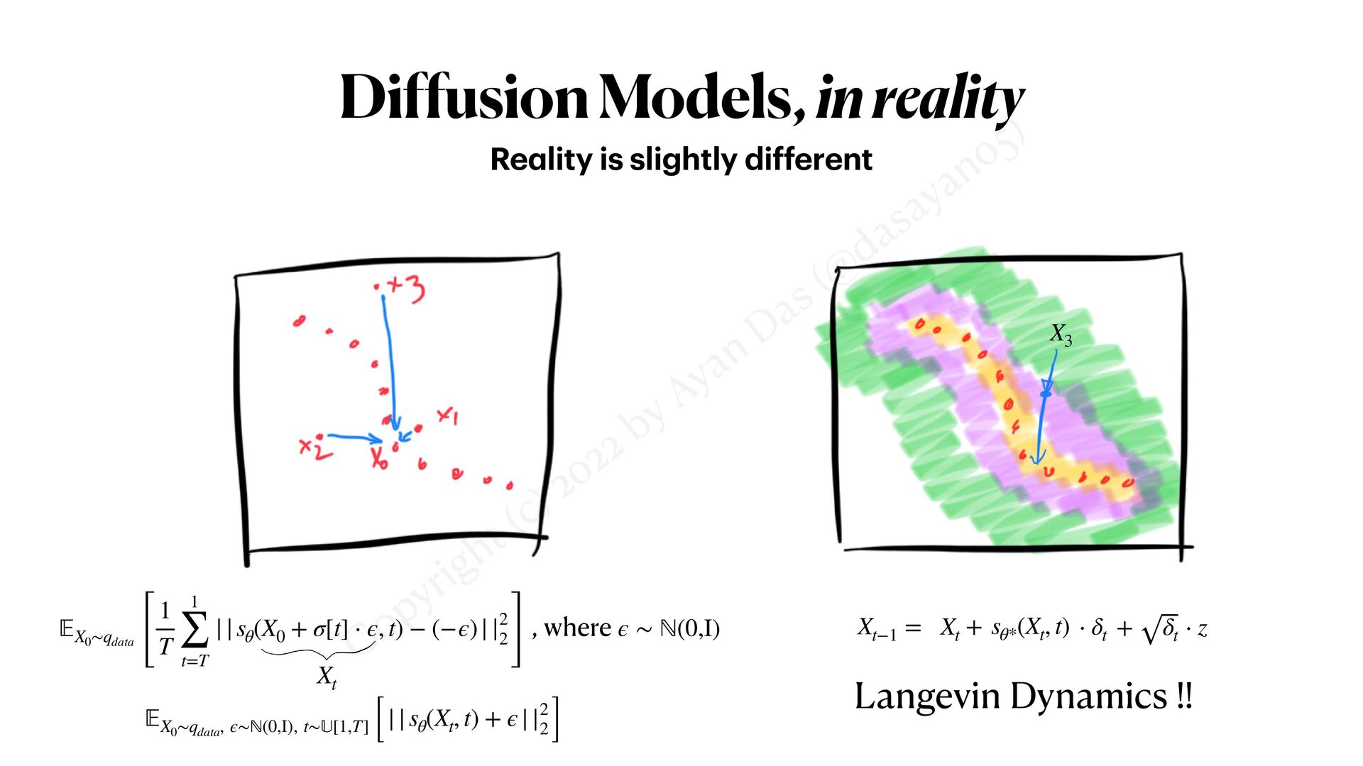
10. Copyright (c) 2022 by Ayan Das (@ dasayan05) Diffusion Models, simpli f ied • Gaussian Di ff usion Model generates data by gradual gaussian de-noising • “Reverse process” is the real generative process • “Forward process” is just a way of simulating noisy training data for all t Intuitive Ide a XT Xt Xt−1 X0 ⋯ ⋯ 𝔼 X0 ∼qdata [ 1 T 1 ∑ t=T ||sθ (Xt ) − Xt−1 ||2 2 ] X0 ⋯ ⋯ Xt Xt−1 XT
11. Copyright (c) 2022 by Ayan Das (@ dasayan05) “Forward-Reverse process is equivalent to VAE-like Encoder-Decoder” WRONG
12. Copyright (c) 2022 by Ayan Das (@ dasayan05) Forward process is “parallelizable” X0 ⋯ ⋯ Xt Xt−1 XT X0 ⋯ ⋯ Xt Xt−1 XT X1 Xt = X0 + σ[t] ⋅ ϵ, where ϵ ∼ ℕ(0, I) σ[t]
13. Copyright (c) 2022 by Ayan Das (@ dasayan05) Diffusion Models, simpli f ied Visu a lising the d a t a sp a ce Vector Field that guides towards real data
14. Copyright (c) 2022 by Ayan Das (@ dasayan05) ∇X log qdata (X) ≈ sθ (X, ⋅ ) “Score” of a Distribution .. a n import a nt st a tistic a l qu a ntity X0 +∇X log qdata (X)| X=X0 X1 ←
15. Copyright (c) 2022 by Ayan Das (@ dasayan05) Diffusion Models, in reality Re a lity is slightly different 𝔼 X0 ∼qdata [ 1 T 1 ∑ t=T ||sθ (X0 + σ[t] ⋅ ϵ, t) − (−ϵ)||2 2 ] , where ϵ ∼ ℕ(0,I) Xt 𝔼 X0 ∼qdata , ϵ∼ℕ(0,I), t∼ 𝕌 [1,T] [ ||sθ (Xt , t) + ϵ||2 2 ] X3 Xt + sθ* (Xt , t) ⋅ δt + δt ⋅ z Xt−1 = Langevin Dynamics !!
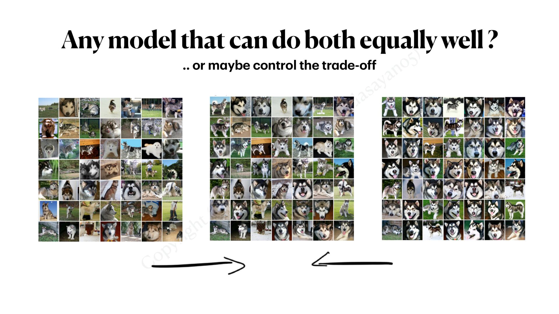
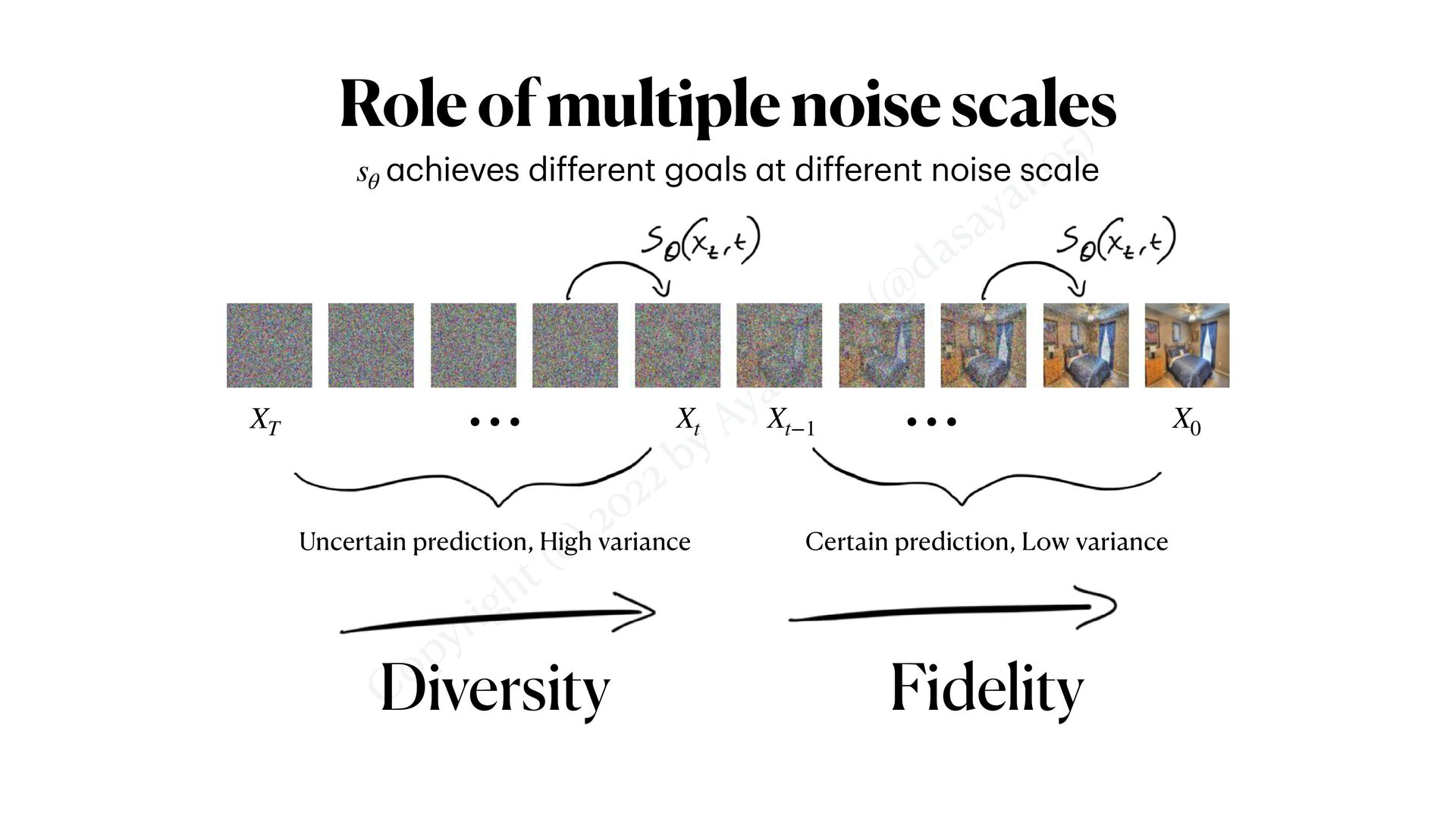
16. Copyright (c) 2022 by Ayan Das (@ dasayan05) Role of multiple noise scales a chieves different go a ls a t different noise sc a le sθ XT Xt Xt−1 X0 ⋯ ⋯ Uncertain prediction, High variance Certain prediction, Low variance Diversity Fidelity
17. Copyright (c) 2022 by Ayan Das (@ dasayan05) Origin Story & Formalisms
18. Copyright (c) 2022 by Ayan Das (@ dasayan05) Tracing Diffusion Model back into history .. where did it st a rt ? SOTA on CIFAR10 FID 3.14
19. Copyright (c) 2022 by Ayan Das (@ dasayan05) Three formalisms SBM, DDPM & SDE De-noising Di ff usion Probabilistic Models (DDPM) Score-Based Models (SBM) Xt−1 = Xt + sθ (Xt , t) ⋅ δt + δt ⋅ z Xt−1 = 1 αt ( Xt − βt 1 − ¯ αt ⋅ ϵθ (Xt , t) ) + σt ⋅ z sθ (Xt , t) = − ϵθ (Xt , t) 1 − ¯ αt Stochastic Di ff erential Equations (SDE) dX = [f(X, t) − g2(t)sθ (X, t)] dt + g(t)dw dw ∼ ℕ(0, dt) f(X, t) = 0 g(t) = d dt σ2(t) f(X, t) = − 1 2 β(t)Xdt g(t) = β(t) Xt−1 = 1 αt (Xt +sθ (Xt , t) ⋅ βt) + βt ⋅ z
20. Copyright (c) 2022 by Ayan Das (@ dasayan05) SBM & DDPM: The important difference • SBM only adds noise • DDPM also scales down the data .. in the forw a rd noising process Xt = X0 + σ[t] ⋅ ϵ, where ϵ ∼ ℕ(0, I) Xt = γ[t] ⋅ X0 + σ[t] ⋅ ϵ, where ϵ ∼ ℕ(0, I) γ[t] = ¯ αt σ[t] = 1 − ¯ αt Xt−1 = Xt + sθ (Xt , t) ⋅ δt + δt ⋅ z SBM: Xt−1 = 1 αt ( Xt − βt 1 − ¯ αt ⋅ ϵθ (Xt , t) ) + σt ⋅ z DDPM:
21. Copyright (c) 2022 by Ayan Das (@ dasayan05) DDPM Summary Forw a rd, Tr a ining a nd Reverse processes Xt = ¯ αt ⋅ X0 + 1 − ¯ αt ⋅ ϵ 𝔼 X0 ∼qdata , ϵ∼ℕ(0,I), t∼ 𝕌 [1,T] [ ||ϵθ(Xt , t) − ϵ||2 2 ] Xt−1 = 1 αt ( Xt − βt 1 − ¯ αt ⋅ ϵθ(Xt , t) ) + σt ⋅ z Sampling from forward process Training the model ϵθ Reverse process sampling with ϵθ*
22. Copyright (c) 2022 by Ayan Das (@ dasayan05) Recent Advancements Faster Sampling
23. Copyright (c) 2022 by Ayan Das (@ dasayan05) Diffusion Models suffer from slow sampling Unlike a ny other gener a tive model Xt−1 = 1 αt ( Xt − βt 1 − ¯ αt ⋅ ϵθ* (Xt , t) ) + σt ⋅ z Xt−1 ∼ 𝒩 (μθ* (Xt , t), σt 2 ⋅ I)
24. Copyright (c) 2022 by Ayan Das (@ dasayan05) De-noising Diffusion Implicit Models (DDIM) F a ster a nd Deterministic s a mpling Xt−1 = ¯ αt−1 ( Xt − 1 − ¯ αt ⋅ ϵθ* (Xt , t) ¯ αt ) + 1 − ¯ αt−1 ϵθ* (Xt , t) Xt−1 ∼ 𝒩 (μDDIM θ* (Xt , t), 0) Stochastic Di ff erential Equation (SDE) Ordinary Di ff erential Equation (SDE)
25. Copyright (c) 2022 by Ayan Das (@ dasayan05) Skip steps in DDIM S a mpling with shorter diffusion length Xt−1 = ¯ αt−1 ( Xt − 1 − ¯ αt ⋅ ϵθ* (Xt , t) ¯ αt ) + 1 − ¯ αt−1 ϵθ* (Xt , t) Xt Xt−1 Xt−k Xt−k = ¯ αt−k ( Xt − 1 − ¯ αt ⋅ ϵθ* (Xt , t) ¯ αt ) + 1− ¯ αt−k ϵθ* (Xt , t)
26. Copyright (c) 2022 by Ayan Das (@ dasayan05) DDIM as feature extractor Deterministic M a pping Xt = ¯ αt−1 ( Xt−1 − 1 − ¯ αt ⋅ ϵθ* (Xt−1 , t) ¯ αt ) + 1 − ¯ αt−1 ϵθ* (Xt−1 , t) ∀t = 0 → T Feature Extractor Initial Value Problem (IVP) Final Value Problem (FVP)
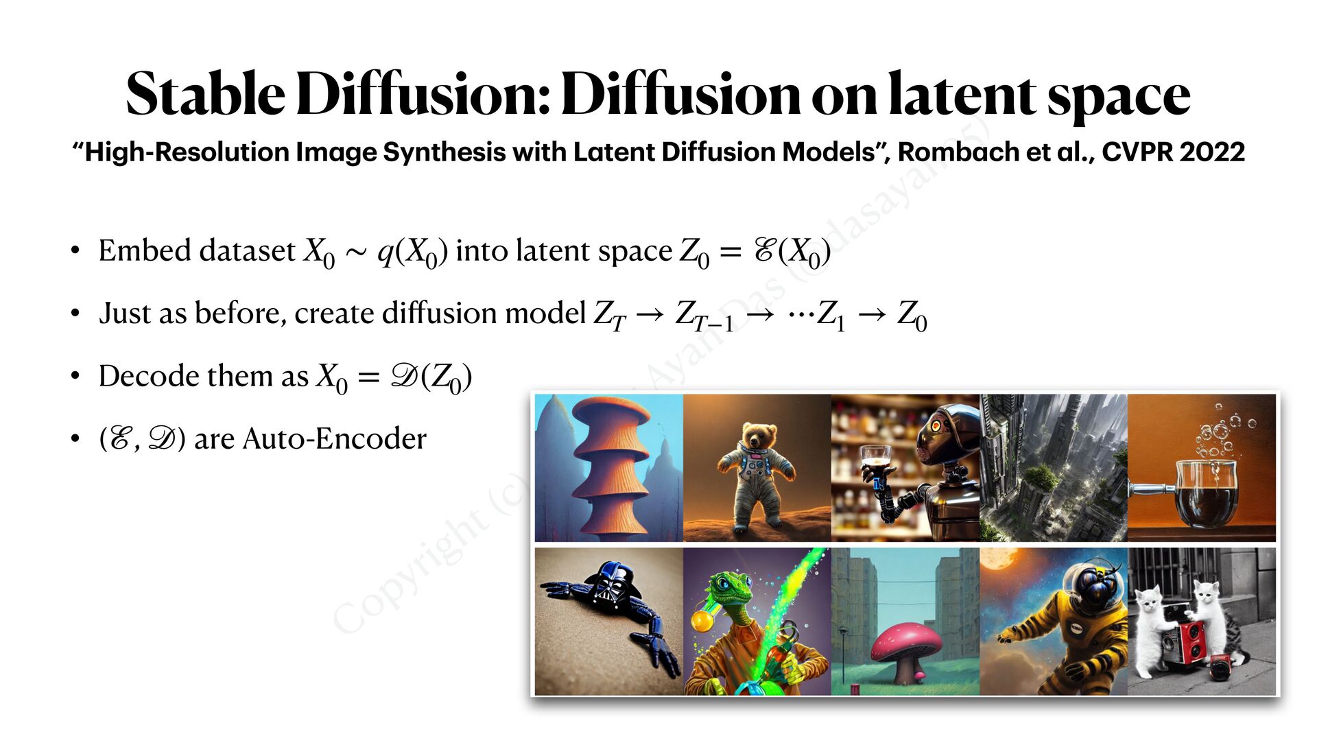
27. Copyright (c) 2022 by Ayan Das (@ dasayan05) Stable Diffusion: Diffusion on latent space • Embed dataset into latent space • Just as before, create di ff usion model • Decode them as • ( , ) are Auto-Encoder X0 ∼ q(X0 ) Z0 = ℰ(X0 ) ZT → ZT−1 → ⋯Z1 → Z0 X0 = 𝒟 (Z0 ) ℰ 𝒟 “High-Resolution Im a ge Synthesis with L a tent Diffusion Models”, Romb a ch et a l., CVPR 2022
28. Copyright (c) 2022 by Ayan Das (@ dasayan05) Recent Advancements Guidance
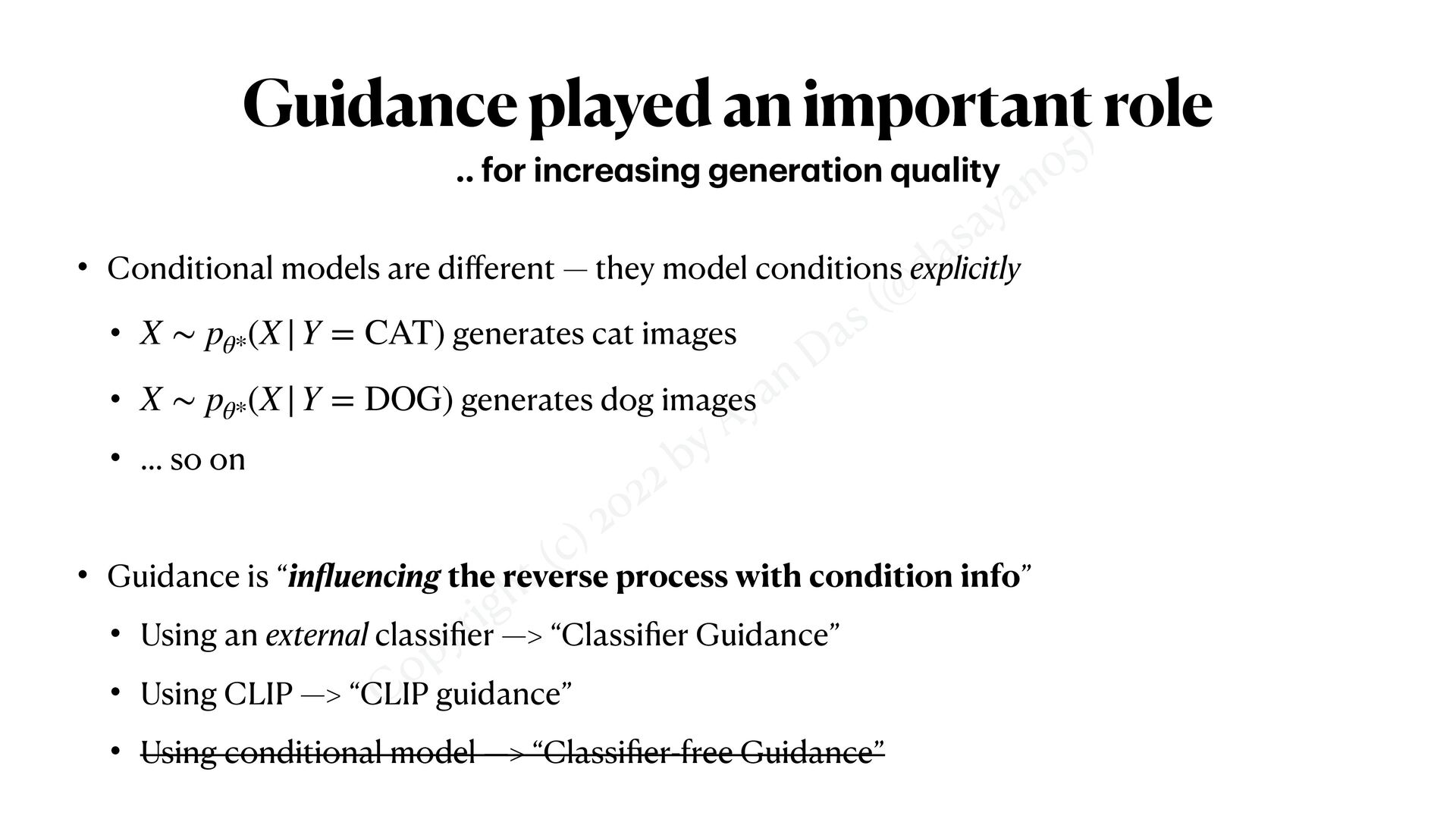
29. Copyright (c) 2022 by Ayan Das (@ dasayan05) Guidance played an important role • Conditional models are di ff erent — they model conditions explicitly • generates cat images • generates dog images • … so on • Guidance is “in fl uencing the reverse process with condition info” • Using an external classi fi er —> “Classi fi er Guidance” • Using CLIP —> “CLIP guidance” • Using conditional model —> “Classi fi er-free Guidance” X ∼ pθ* (X|Y = CAT) X ∼ pθ* (X|Y = DOG) .. for incre a sing gener a tion qu a lity
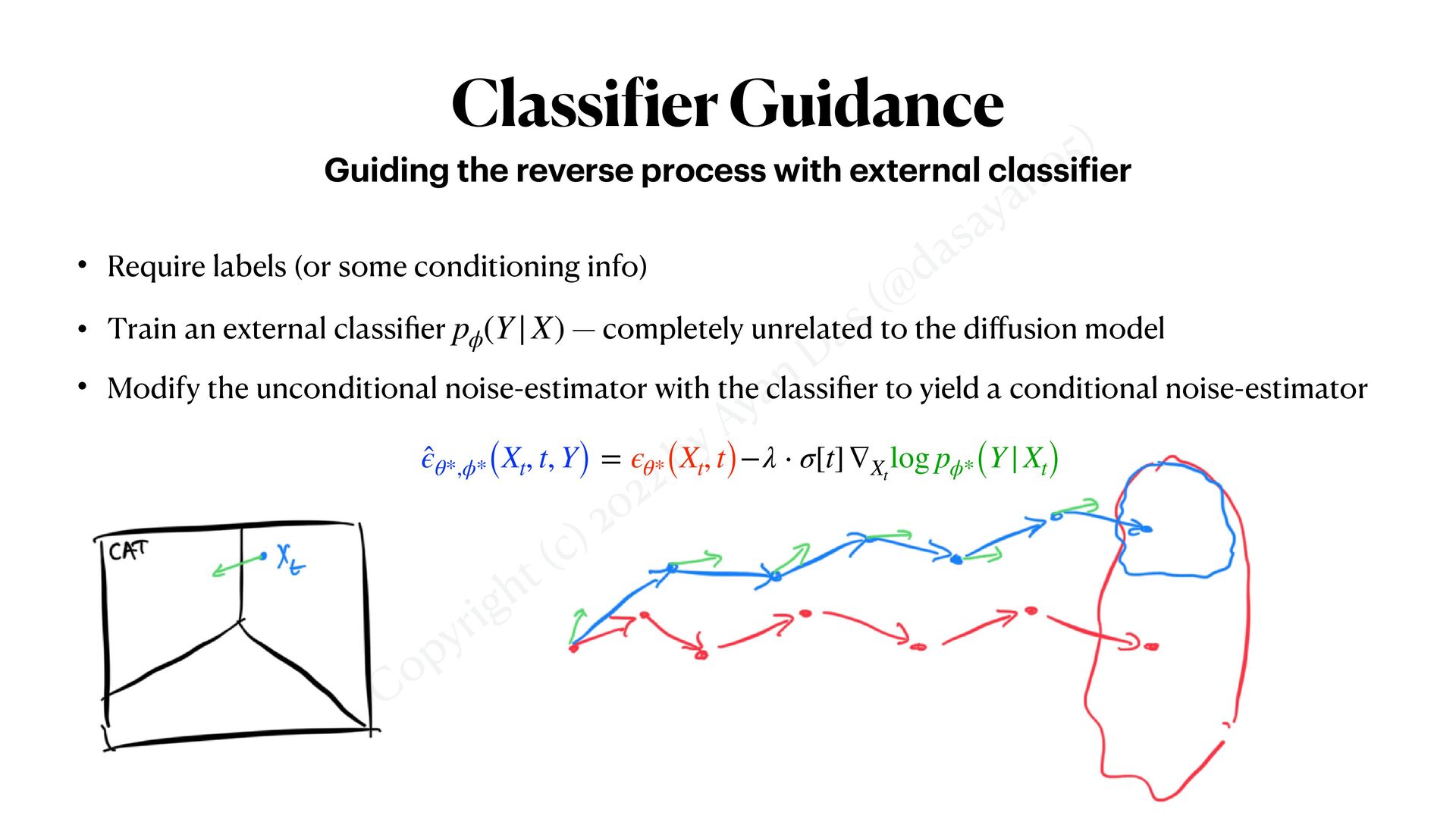
30. Copyright (c) 2022 by Ayan Das (@ dasayan05) Classi f ier Guidance • Require labels (or some conditioning info) • Train an external classi fi er — completely unrelated to the di ff usion model • Modify the unconditional noise-estimator with the classi fi er to yield a conditional noise-estimator pϕ (Y|X) Guiding the reverse process with extern a l cl a ssi f ier ̂ ϵθ*,ϕ*(Xt , t, Y) = ϵθ*(Xt , t)−λ ⋅ σ[t]∇Xt log pϕ*(Y|Xt)
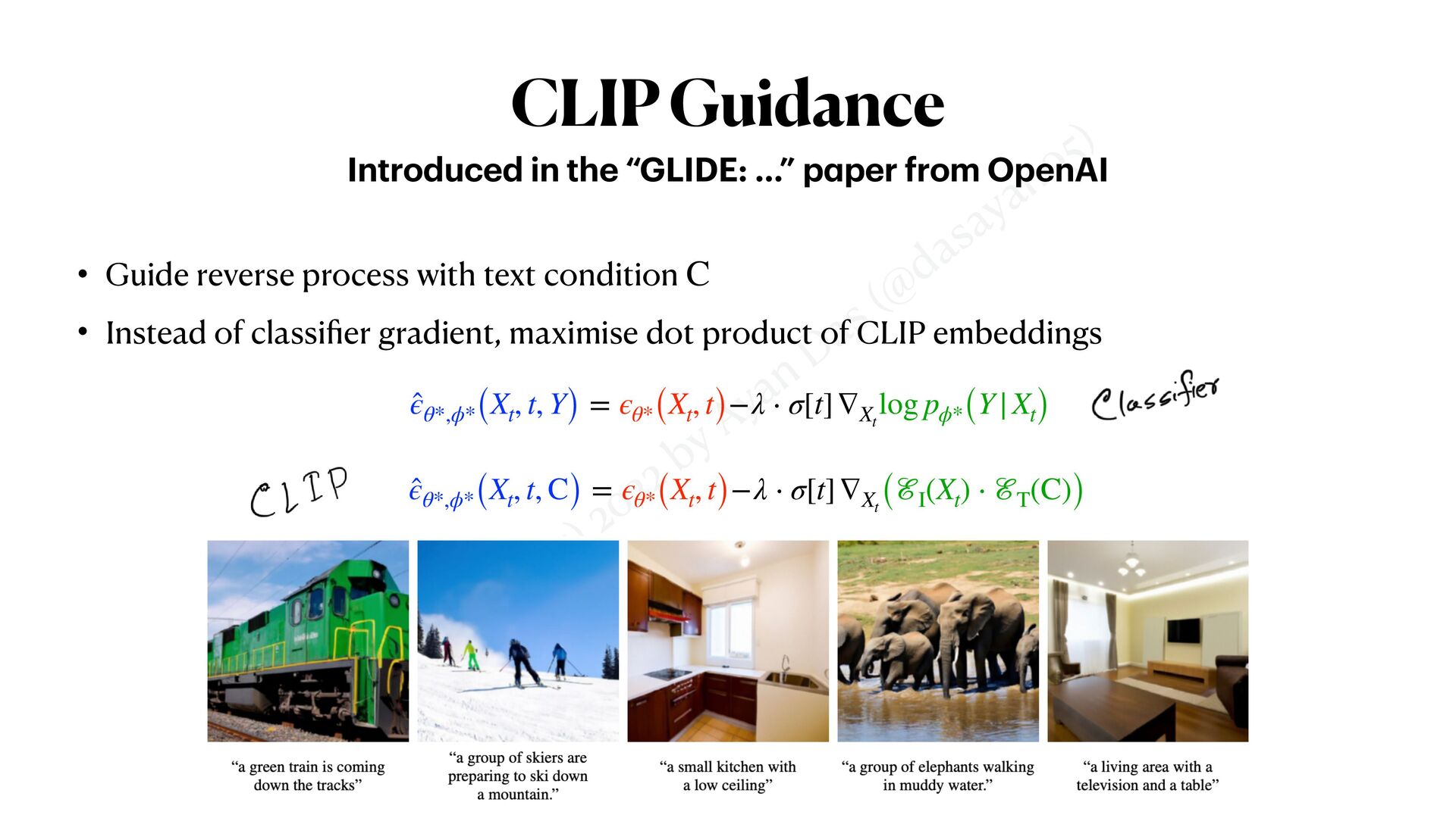
31. Copyright (c) 2022 by Ayan Das (@ dasayan05) CLIP Guidance • Guide reverse process with text condition • Instead of classi fi er gradient, maximise dot product of CLIP embeddings C Introduced in the “GLIDE: …” p a per from OpenAI ̂ ϵθ*,ϕ*(Xt , t, Y) = ϵθ*(Xt , t)−λ ⋅ σ[t]∇Xt log pϕ*(Y|Xt) ̂ ϵθ*,ϕ*(Xt , t, C) = ϵθ*(Xt , t)−λ ⋅ σ[t]∇Xt (ℰI (Xt ) ⋅ ℰT (C))
32. Copyright (c) 2022 by Ayan Das (@ dasayan05) Recent Application Conditional Models
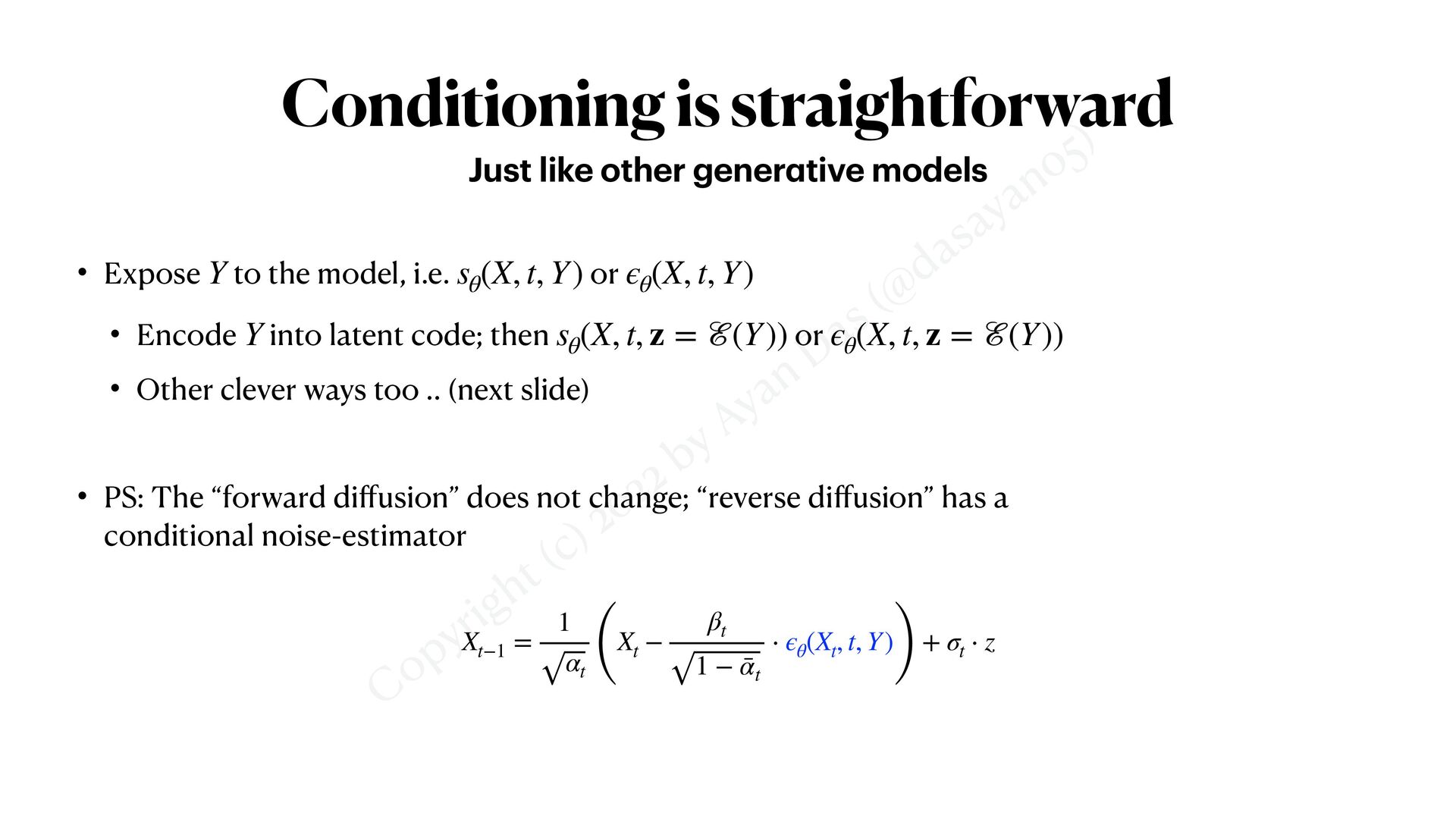
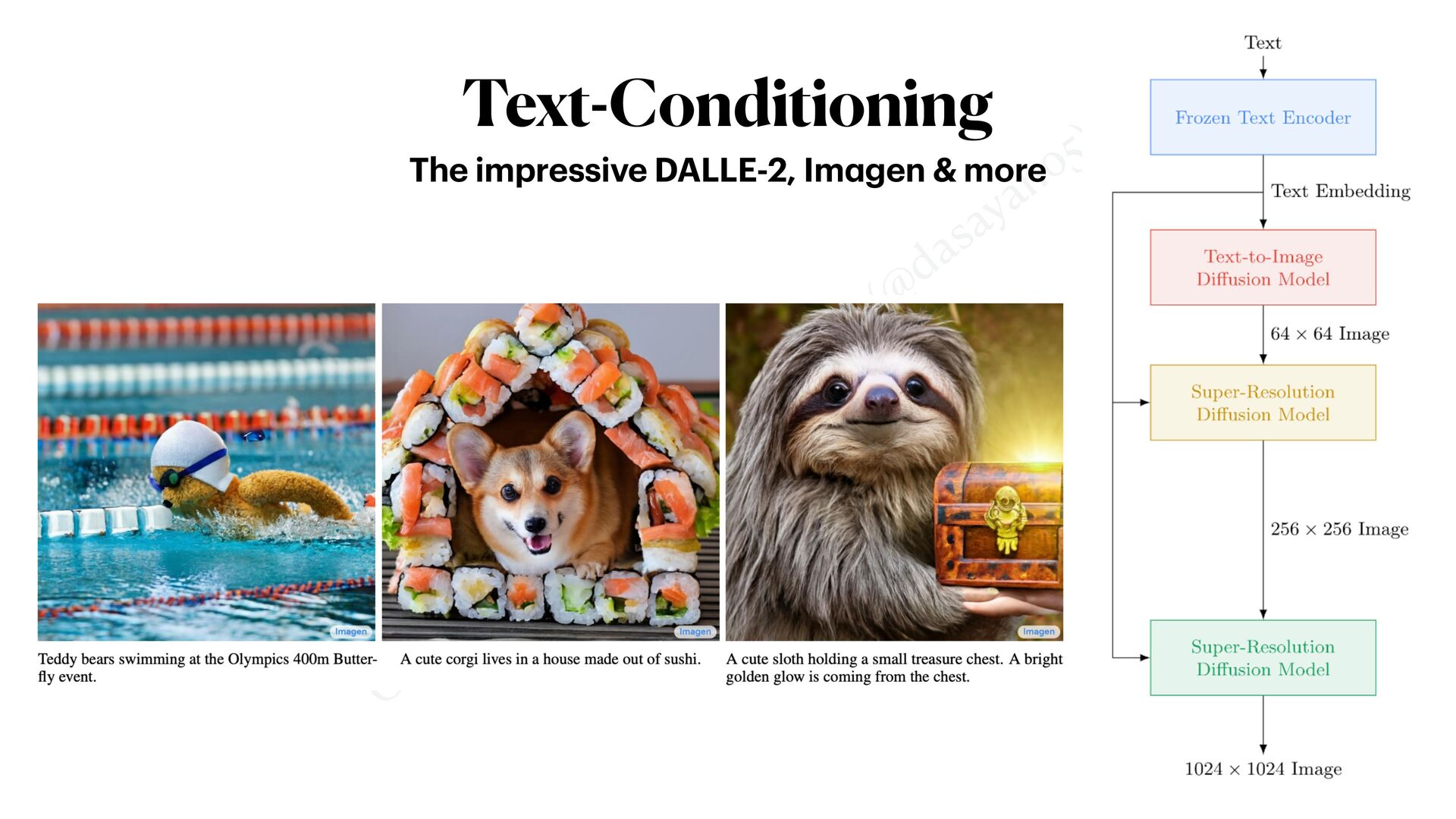
33. Copyright (c) 2022 by Ayan Das (@ dasayan05) Conditioning is straightforward • Expose to the model, i.e. or • Encode into latent code; then or • Other clever ways too .. (next slide) • PS: The “forward di ff usion” does not change; “reverse di ff usion” has a 
 conditional noise-estimator Y sθ (X, t, Y) ϵθ (X, t, Y) Y sθ (X, t, z = ℰ(Y)) ϵθ (X, t, z = ℰ(Y)) Just like other gener a tive models Xt−1 = 1 αt ( Xt − βt 1 − ¯ αt ⋅ ϵθ (Xt , t, Y) ) + σt ⋅ z
34. Copyright (c) 2022 by Ayan Das (@ dasayan05) Text-Conditioning The impressive DALLE-2, Im a gen & more
35. Copyright (c) 2022 by Ayan Das (@ dasayan05) “Super-Resolution” with Conditional Diffusion “Im a ge Super-Resolution vi a Iter a tive Re f inement”, S a h a ri a et a l. Y ∼ pθ (X|Y) Xt−1 ∼ pθ (Xt−1 |Xt , Y) Y
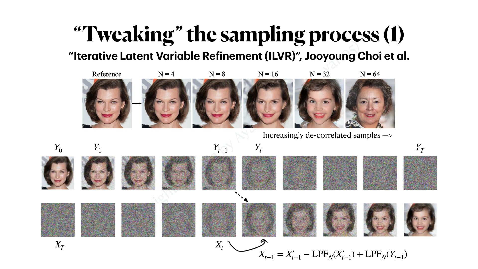
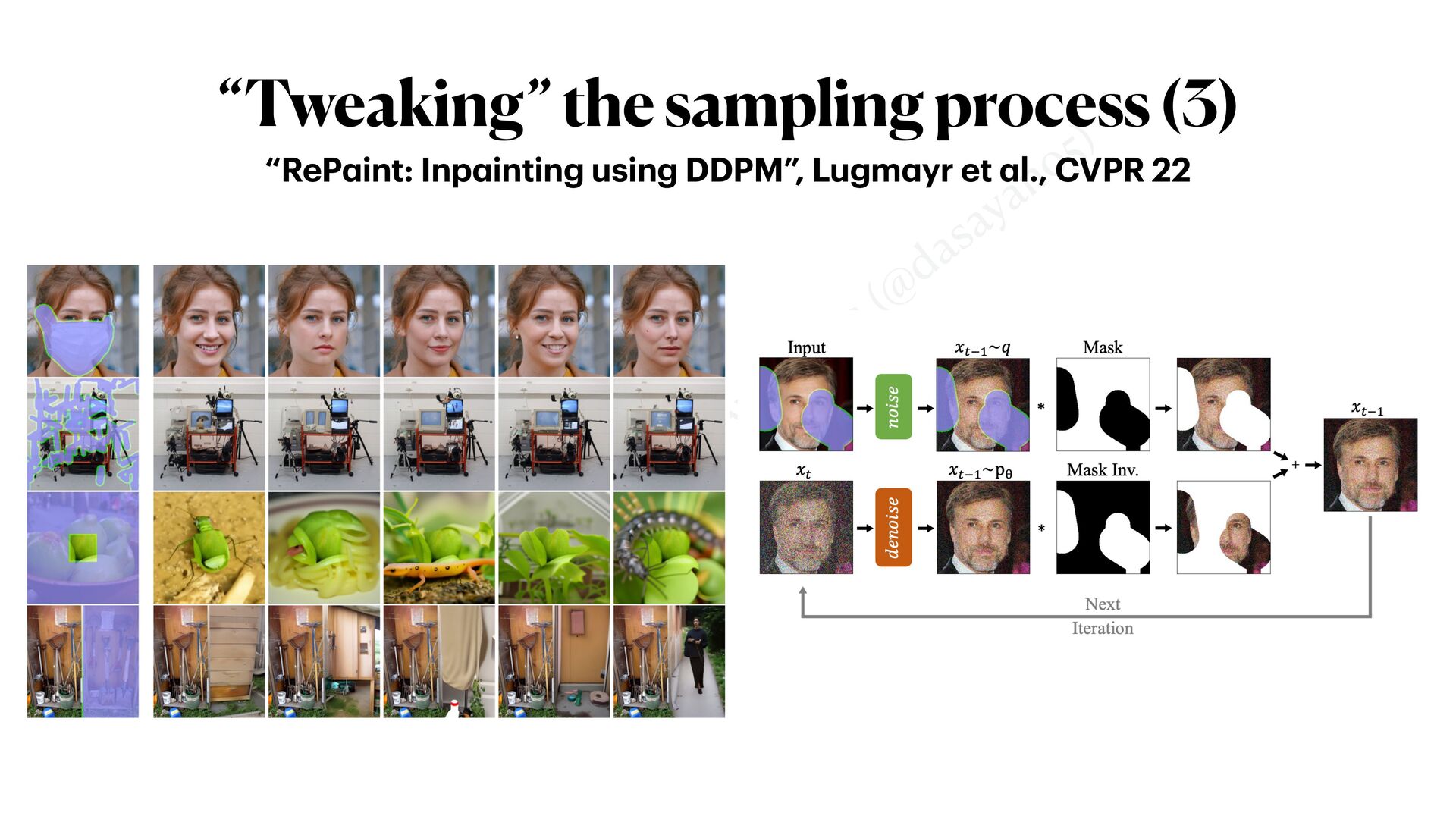
36. Copyright (c) 2022 by Ayan Das (@ dasayan05) “Tweaking” the sampling process (1) “Iter a tive L a tent V a ri a ble Re f inement (ILVR)”, Jooyoung Choi et a l. Increasingly de-correlated samples —> Y0 Y1 Yt−1 YT Yt Xt−1 = X′  t−1 − LPFN (X′  t−1 ) + LPFN (Yt−1 ) XT Xt
37. Copyright (c) 2022 by Ayan Das (@ dasayan05) “Tweaking” the sampling process (2) “SDEdit: Guided im a ge synthesis …”, Chenlin et a l. Forward di ff use the condition —> Y0 Y1 Yt Xt := Yt Xt−1 ∼ pθ (Xt−1 |Xt )
38. Copyright (c) 2022 by Ayan Das (@ dasayan05) “Tweaking” the sampling process (3) “ReP a int: Inp a inting using DDPM”, Lugm a yr et a l., CVPR 22
39. Copyright (c) 2022 by Ayan Das (@ dasayan05) Di ff usion Models .. for other data modalities
40. Copyright (c) 2022 by Ayan Das (@ dasayan05) Forward-Reverse process is quite generic Do not a ssume the structure of the d a t a a nd/or model Xt = ¯ αt ⋅ X0 + 1 − ¯ αt ⋅ ϵ ̂ ϵ ← ϵθ(Xt , t)
41. Copyright (c) 2022 by Ayan Das (@ dasayan05) Molecule : Diffusion on Graphs “Equiv a ri a nt Diffusion for Molecule …”, Hoogeboom et a l., ICML 2022 [Vt , Et] = ¯ αt ⋅ [V0 , E0] + 1 − ¯ αt ⋅ [ϵV , ϵE] [ ̂ ϵV , ̂ ϵE] ← EGNN([Vt , Et], t) N ∑ n=1 V(n) t = 0 Extra requirement for E(3) equivariant graphs
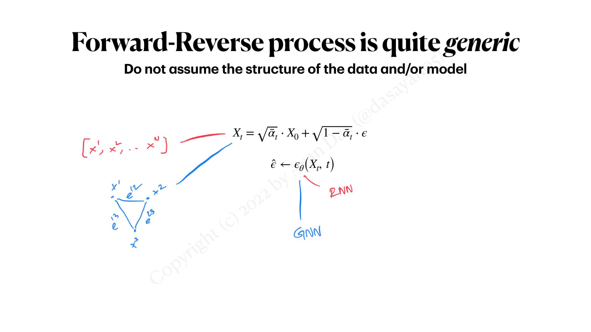
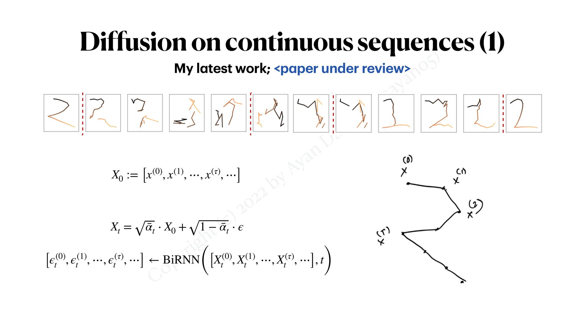
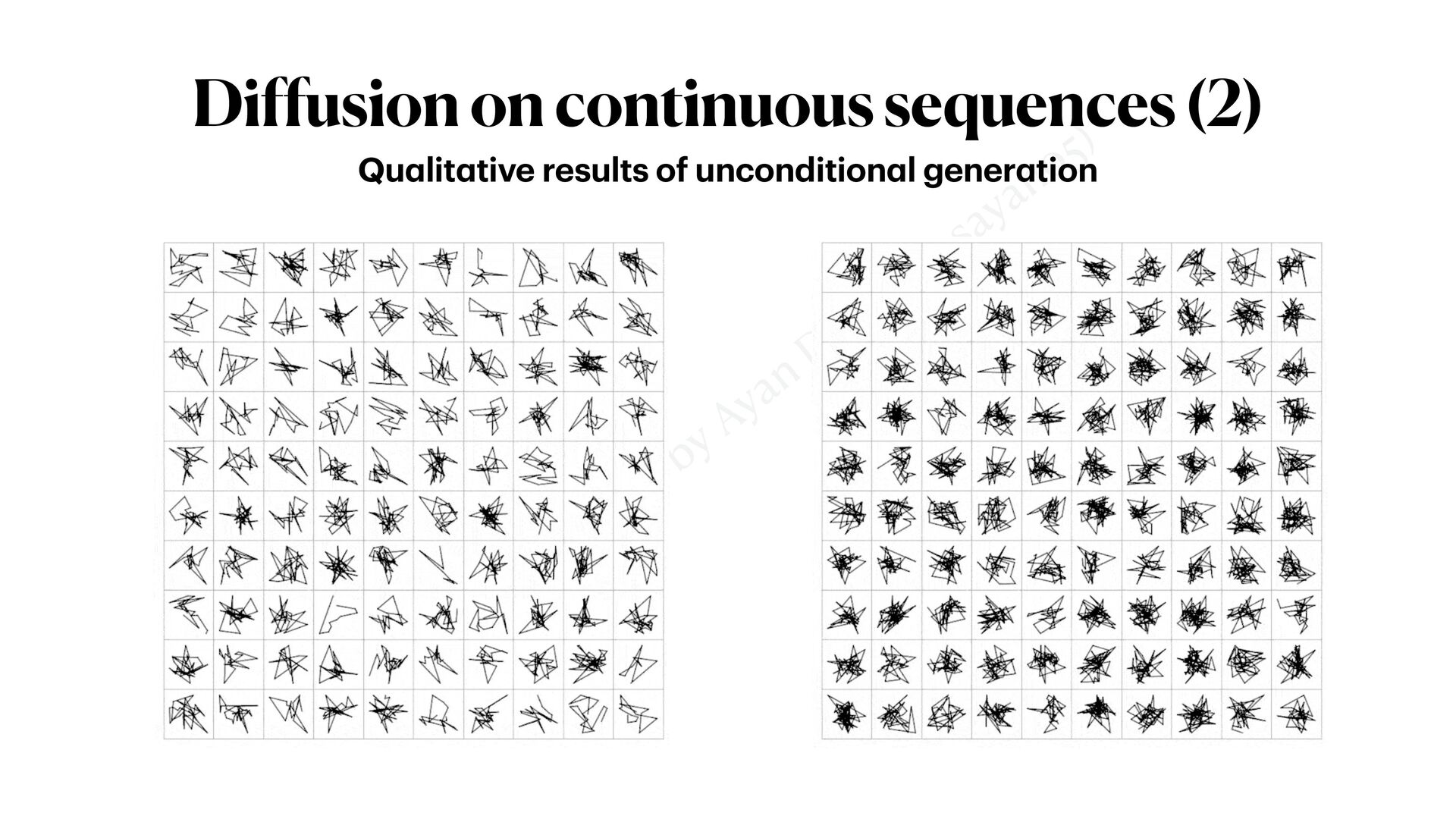
42. Copyright (c) 2022 by Ayan Das (@ dasayan05) Diffusion on continuous sequences (1) My l a test work; <p a per under review> X0 := [x(0), x(1), ⋯, x(τ), ⋯] Xt = ¯ αt ⋅ X0 + 1 − ¯ αt ⋅ ϵ [ϵ(0) t , ϵ(1) t , ⋯, ϵ(τ) t , ⋯] ← BiRNN([X(0) t , X(1) t , ⋯, X(τ) t , ⋯], t)
43. Copyright (c) 2022 by Ayan Das (@ dasayan05) Diffusion on continuous sequences (2) Qu a lit a tive results of uncondition a l gener a tion
44. Questions ? @d a s a y a n05 https:// a y a nd a s.me/ a .d a s@surrey. a c.uk