Detecting Asteroids with Neural Networks

See https://github.com/di/astro

Transcript

1. Detecting Asteroids with Neural Networks Dustin Ingram Advanced Artificial Intelligence, Winter 12-13 Drexel University Department of Computer Science March 10, 2013
2. Outline What’s the goal? What’s the data? Getting started Building a feature set Building the neural network Training the network Results
3. The goal Build and train a neural network to correctly identify asteroids in astrophotography data.
4. So... How do we do it?
5. So... How do we really do it?
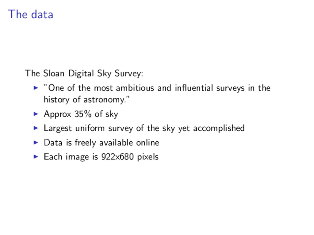
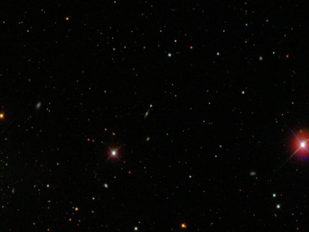
6. The data The Sloan Digital Sky Survey: ”One of the most ambitious and influential surveys in the history of astronomy.” Approx 35% of sky Largest uniform survey of the sky yet accomplished Data is freely available online Each image is 922x680 pixels
9. An example asteroid
10. An example asteroid
11. How does this work? This exploits a property of CCDs: SDSS telescopes use five different filters They are not simultaneous Moving objects appear in different locations Always the same order
12. An example asteroid
13. Getting started Getting the initial training data: Small tool to extract potential candidates from full-scale images Extremely na¨ ıve, approx 100:5 false positives to actual positives Very low false negatives (approx 1:1000) Incredibly slow (complex scan of 100Ks of potentials) Manual classification, somewhat slow Yields approx 250 valid items, 500 invalid items
14. The feature set Good ideas for features: Ratio valid hues to non-valid hues Best possible cluster collinearity Best possible average cluster distance
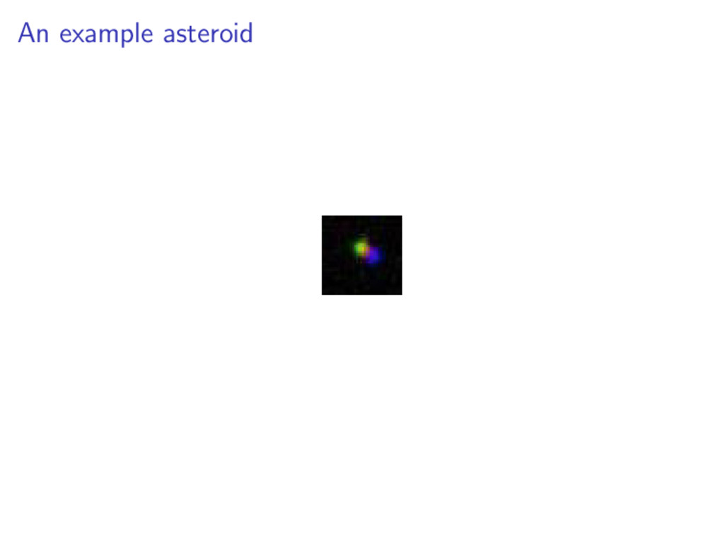
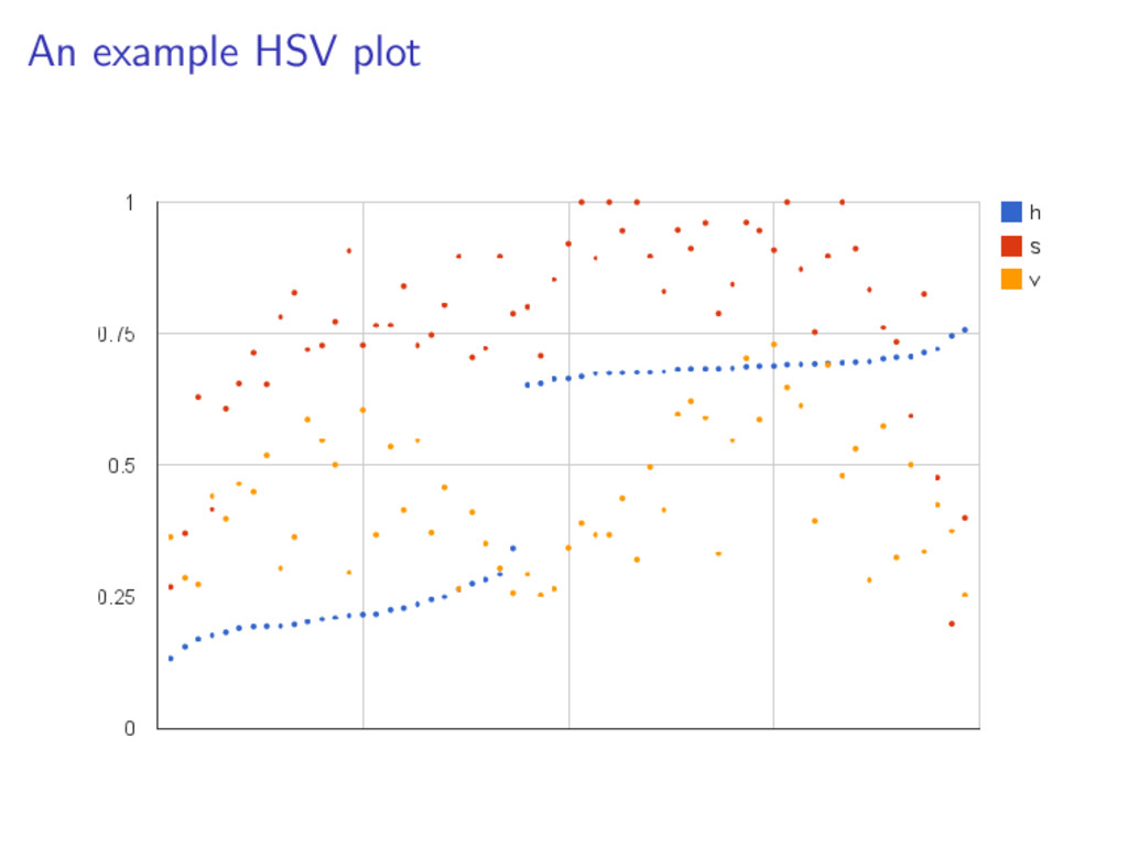
15. Feature: Ratio valid hues to non-valid hues The goal here is to match the colors, a.k.a. “hues”: First step: convert to HSV space For pixels in the valid value-spectrum (0.25 < v < 0.90) How many are within 2 standard deviations from an optimal value? What’s the ratio to ones that aren’t?
16. An example HSV plot
17. Feature: Best possible cluster collinearity k-means clustering Using the valid hues from the previous feature Attempts to cluster n points into k groups Here, k = 3 Produces three centroids
18. An example asteroid
19. k-means clustering of the same asteroid
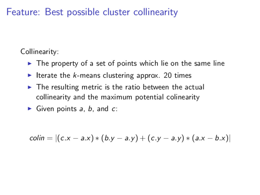
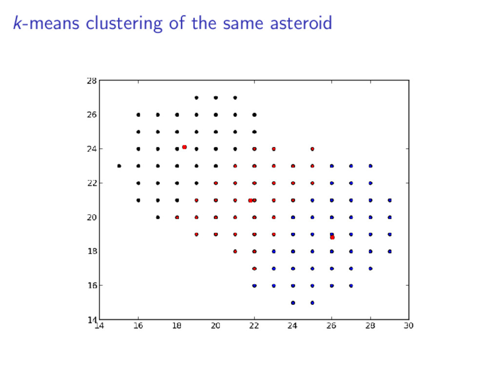
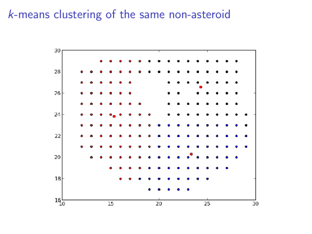
20. Feature: Best possible cluster collinearity Collinearity: The property of a set of points which lie on the same line Iterate the k-means clustering approx. 20 times The resulting metric is the ratio between the actual collinearity and the maximum potential colinearity Given points a, b, and c: colin = |(c.x − a.x) ∗ (b.y − a.y) + (c.y − a.y) ∗ (a.x − b.x)|
21. An example asteroid
22. k-means clustering of the same asteroid
23. An example non-asteroid
24. k-means clustering of the same non-asteroid
25. Feature: Best possible average cluster distance Using the same k-means clusters from the previous features What is the average distance from any point in a cluster to the center of the cluster?
26. An example asteroid
27. k-means clustering of the same asteroid
28. An example non-asteroid
29. k-means clustering of the same non-asteroid
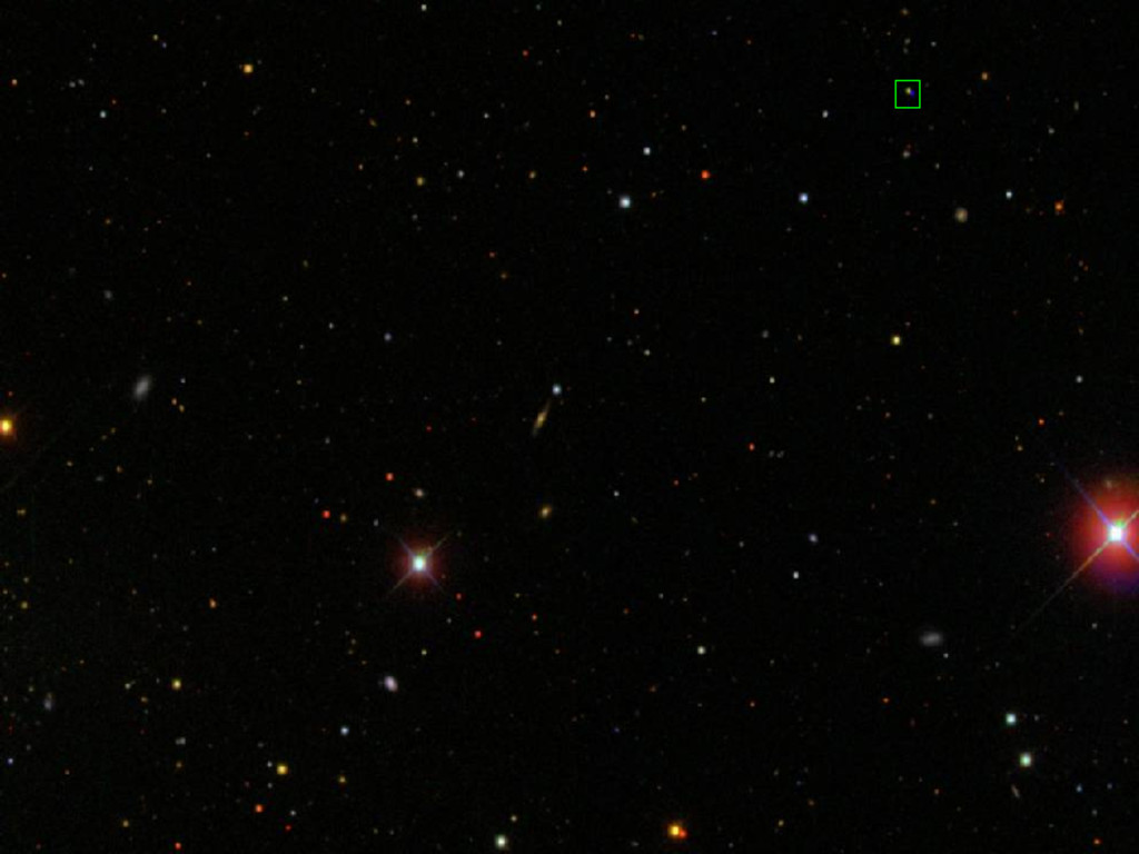
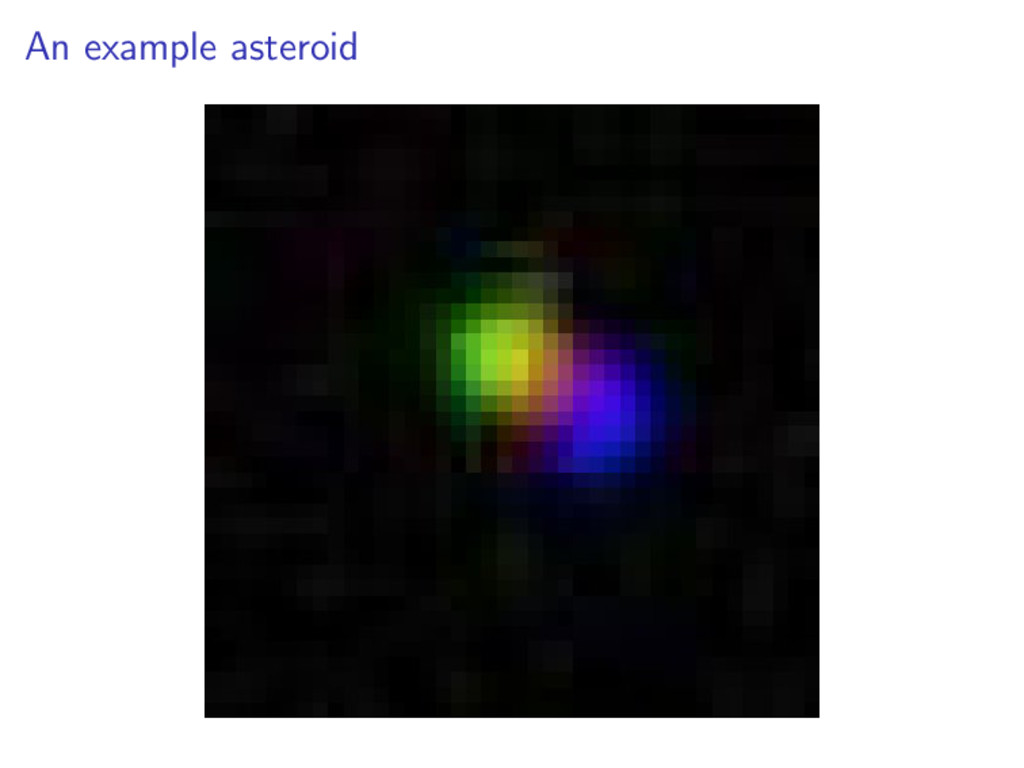
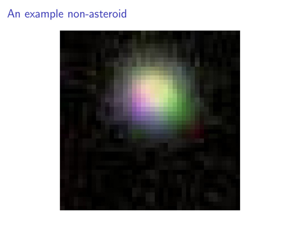
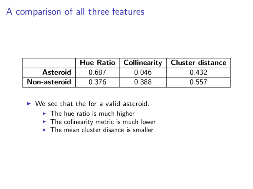
30. A comparison of all three features Hue Ratio Collinearity Cluster distance Asteroid 0.687 0.046 0.432 Non-asteroid 0.376 0.388 0.557 We see that the for a valid asteroid: The hue ratio is much higher The colinearity metric is much lower The mean cluster disance is smaller
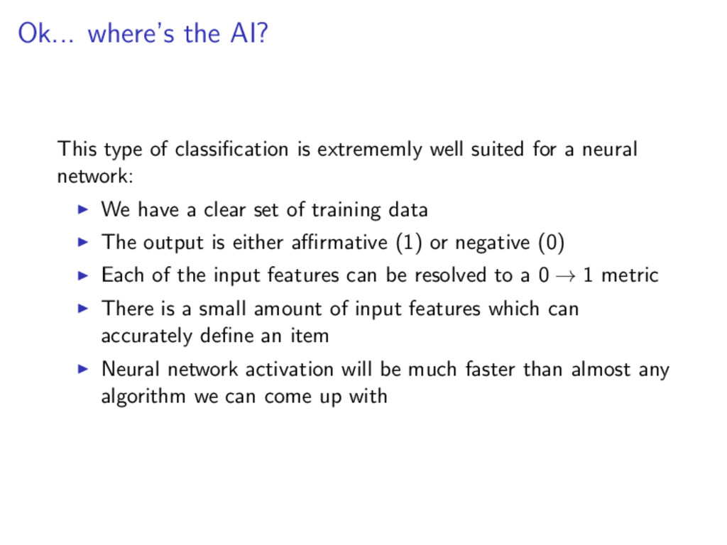
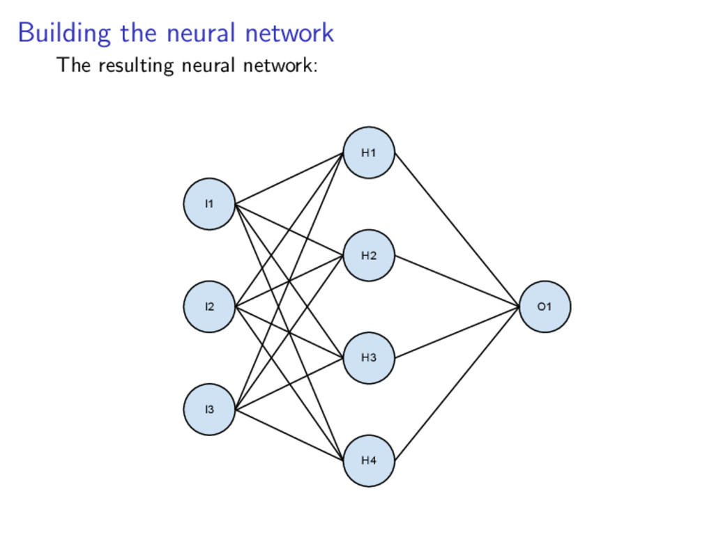
31. Ok... where’s the AI? This type of classification is extrememly well suited for a neural network: We have a clear set of training data The output is either affirmative (1) or negative (0) Each of the input features can be resolved to a 0 → 1 metric There is a small amount of input features which can accurately define an item Neural network activation will be much faster than almost any algorithm we can come up with
32. Building the neural network The resulting neural network: Use supervised learning Uses a backpropagation trainer Three layers: Input layer Single hidden layer Output layer Total of 8 “neurons”: 3 input neurons (hue ratio, collinearity metric, distance metric) 4 hidden neurons 1 output neuron (1 if valid asteroid, 0 if invalid) Learning rate of 0.01, momentum of 0.99
33. Building the neural network The resulting neural network: I1 I2 I3 H1 H2 H3 H4 O1
34. Training the network Approx 250 valid items Approx 500 invalid items Trained for 5,000 iterations Took approx. 3 hours Probably could have gotten by with less iterations
35. Results Trial Found Valid Actual Valid Total False positive Trial 1 8 5 190 37.50% Trial 2 23 21 286 8.70% Trial 3 54 46 955 14.81%
36. Results Trial Found Invalid Actual Invalid Total False negative Trial 1 182 182 190 0.00% Trial 2 263 262 286 0.38% Trial 3 901 892 955 1.00%
37. Conclusion Using a neural network allows us to do it faster, and more accurately Need to spend time coming up with good features for the data When paired with human validation, the process would become very quick and very accurate
38. References http://www.sdss.org/ http://pybrain.org/ http://en.wikipedia.org/wiki/Sloan_Digital_Sky_Survey http://en.wikipedia.org/wiki/Collinearity http://en.wikipedia.org/wiki/K-means_clustering