Dan Weisz University of Washington Hubble Fellow Charlie Conroy (CfA) Ben Johnson (CfA) Dan Foreman-Mackey (UW) David W. Hogg (NYU) Galaxy Coffee MPIA 6.8.2015
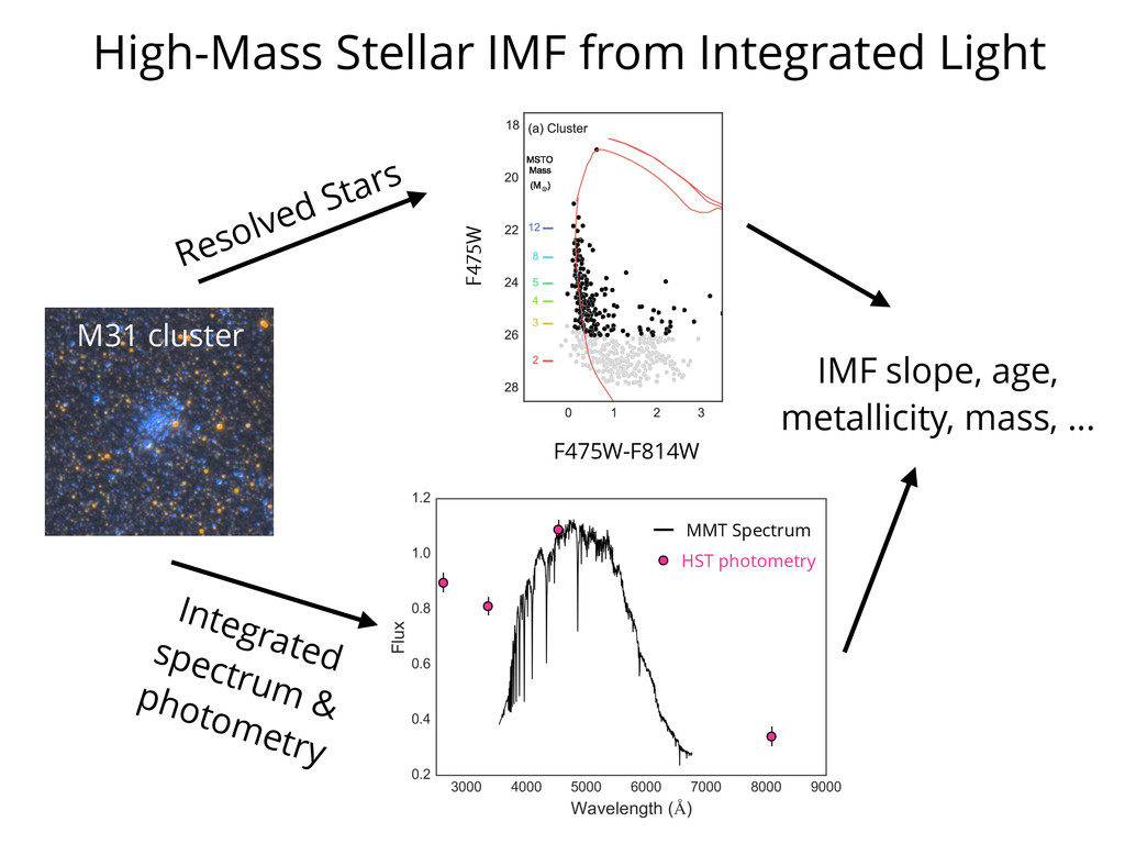
and photometry: want to use all information. ‣ Spectrum contains more information than photometry, but suffers from systematics. M31 cluster HST photometry MMT Spectrum
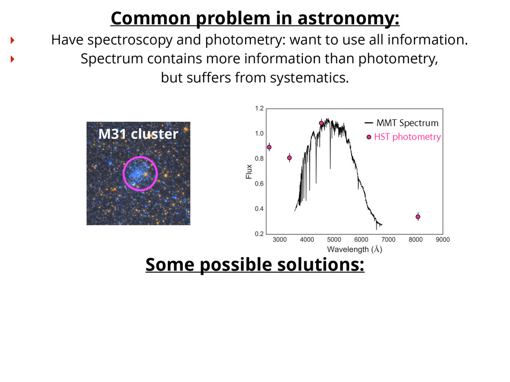
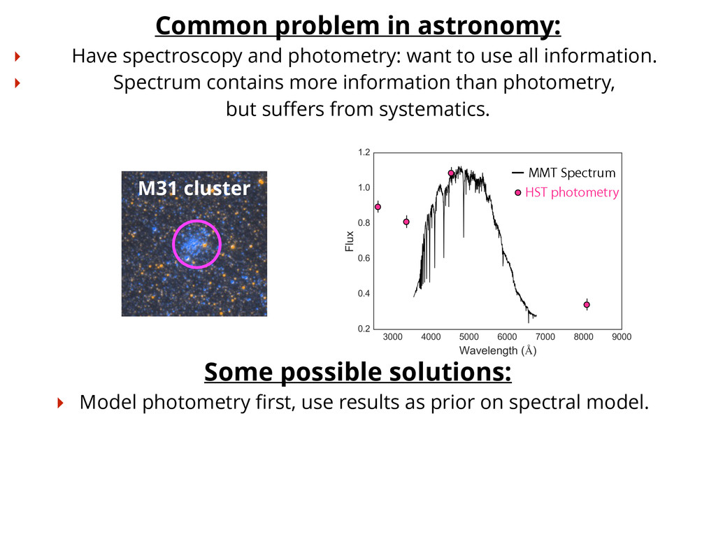
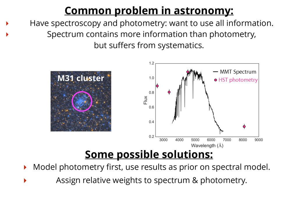
prior on spectral model. Common problem in astronomy: ‣ Have spectroscopy and photometry: want to use all information. ‣ Spectrum contains more information than photometry, but suffers from systematics. M31 cluster HST photometry MMT Spectrum
prior on spectral model. ‣ Assign relative weights to spectrum & photometry. Common problem in astronomy: ‣ Have spectroscopy and photometry: want to use all information. ‣ Spectrum contains more information than photometry, but suffers from systematics. M31 cluster HST photometry MMT Spectrum
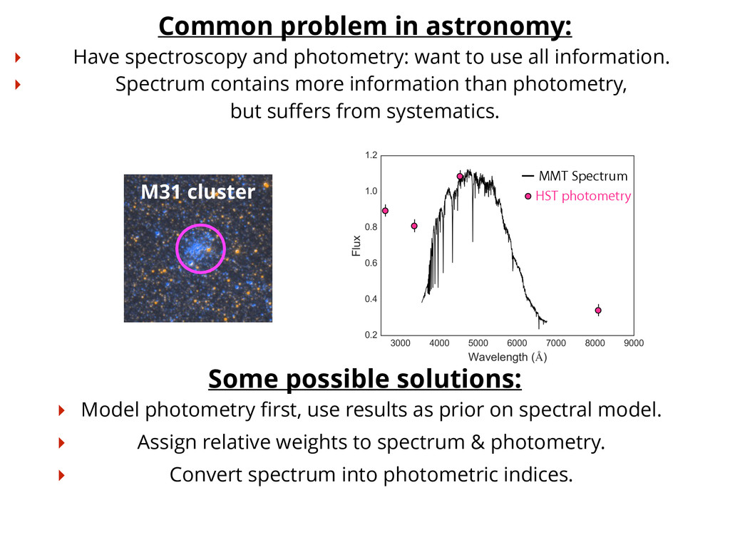
prior on spectral model. ‣ Assign relative weights to spectrum & photometry. ‣ Convert spectrum into photometric indices. Common problem in astronomy: ‣ Have spectroscopy and photometry: want to use all information. ‣ Spectrum contains more information than photometry, but suffers from systematics. M31 cluster HST photometry MMT Spectrum
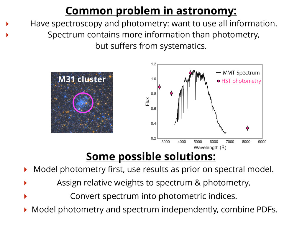
prior on spectral model. ‣ Assign relative weights to spectrum & photometry. ‣ Convert spectrum into photometric indices. ‣ Model photometry and spectrum independently, combine PDFs. Common problem in astronomy: ‣ Have spectroscopy and photometry: want to use all information. ‣ Spectrum contains more information than photometry, but suffers from systematics. M31 cluster HST photometry MMT Spectrum
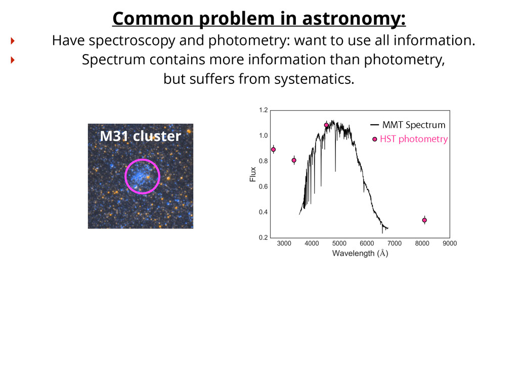
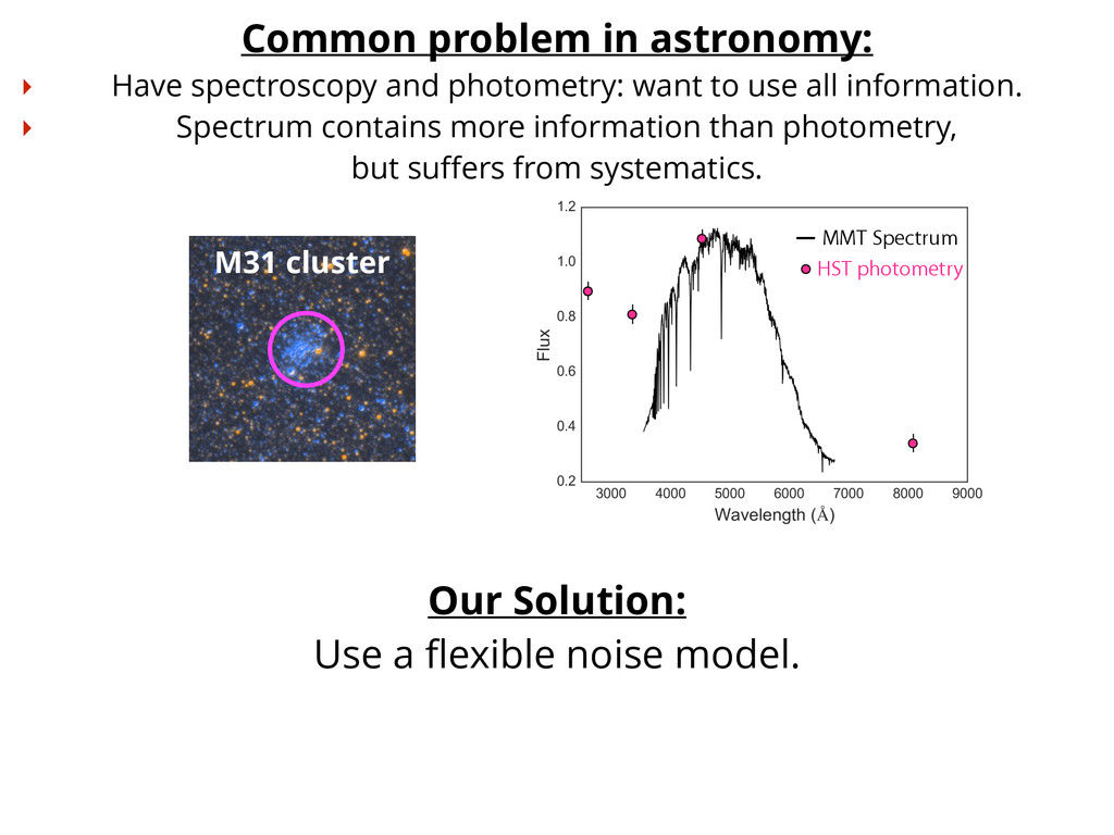
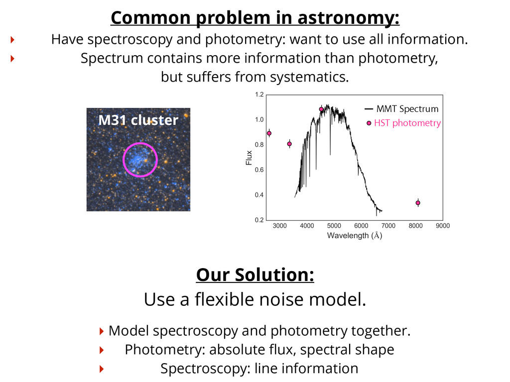
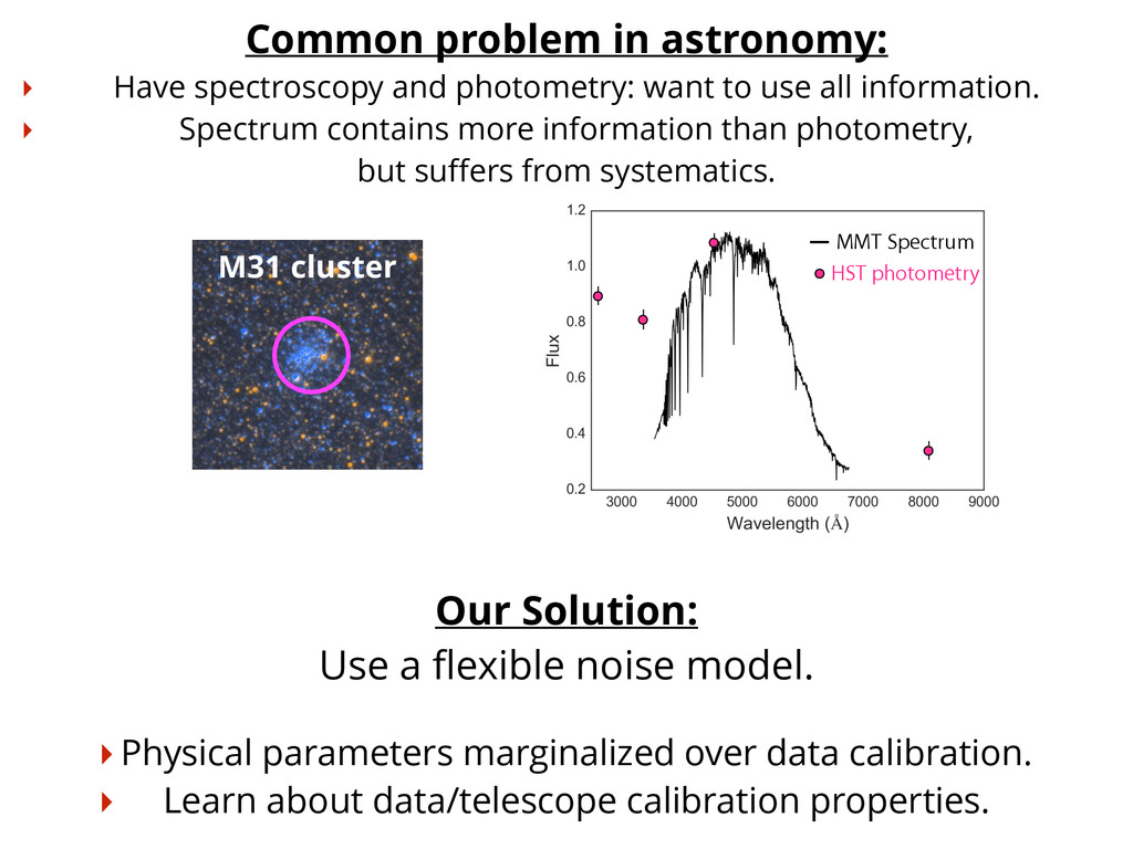
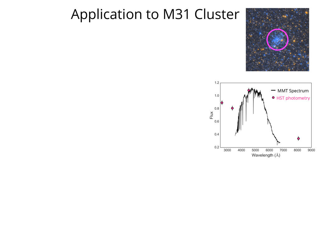
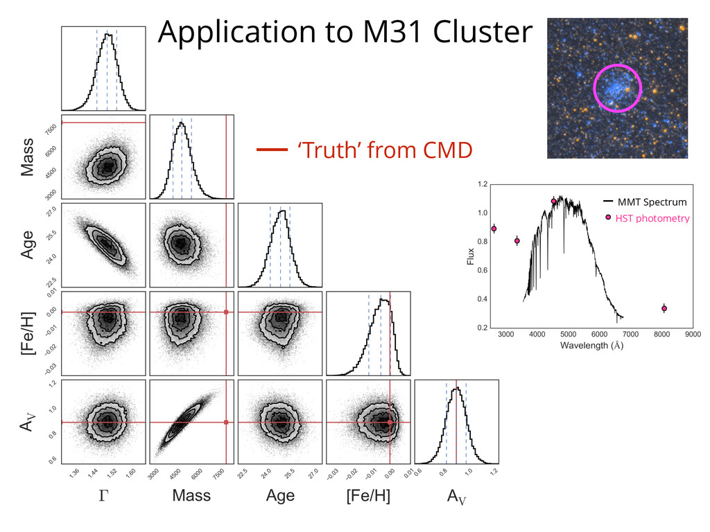
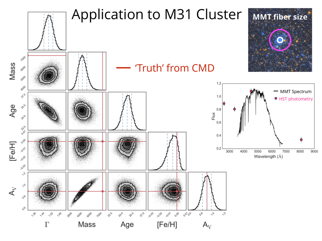
photometry MMT Spectrum Common problem in astronomy: ‣ Have spectroscopy and photometry: want to use all information. ‣ Spectrum contains more information than photometry, but suffers from systematics.
photometry MMT Spectrum ‣ Model spectroscopy and photometry together. ‣ Photometry: absolute flux, spectral shape ‣ Spectroscopy: line information Common problem in astronomy: ‣ Have spectroscopy and photometry: want to use all information. ‣ Spectrum contains more information than photometry, but suffers from systematics.
photometry MMT Spectrum ‣ Physical parameters marginalized over data calibration. ‣ Learn about data/telescope calibration properties. Common problem in astronomy: ‣ Have spectroscopy and photometry: want to use all information. ‣ Spectrum contains more information than photometry, but suffers from systematics.
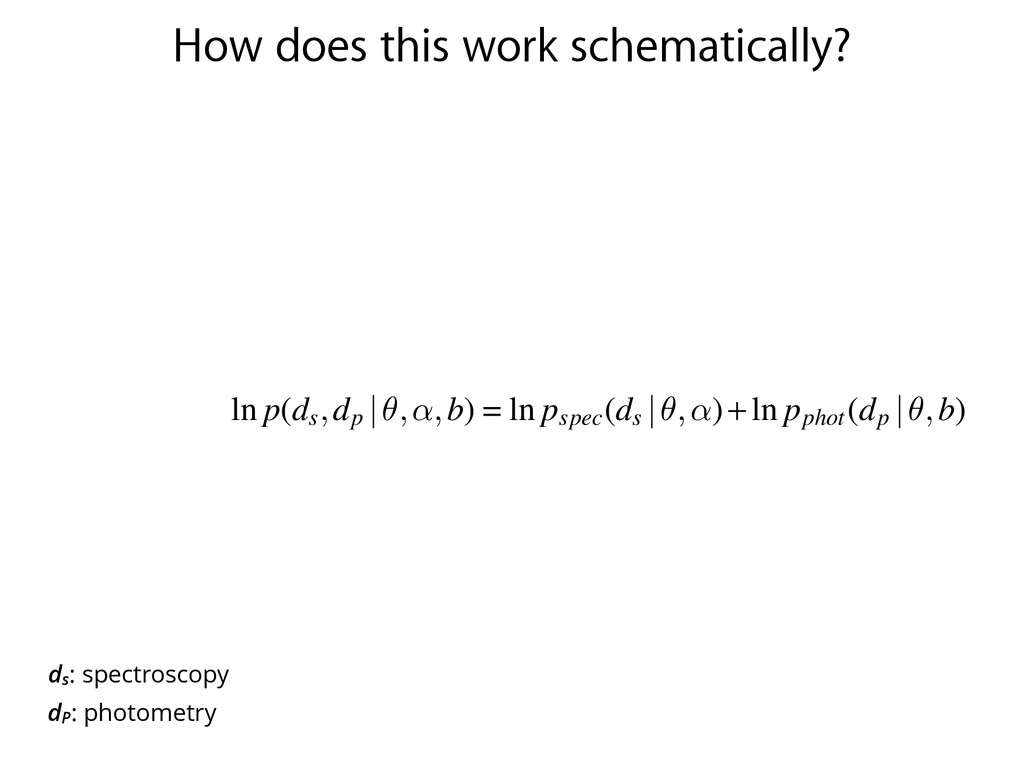
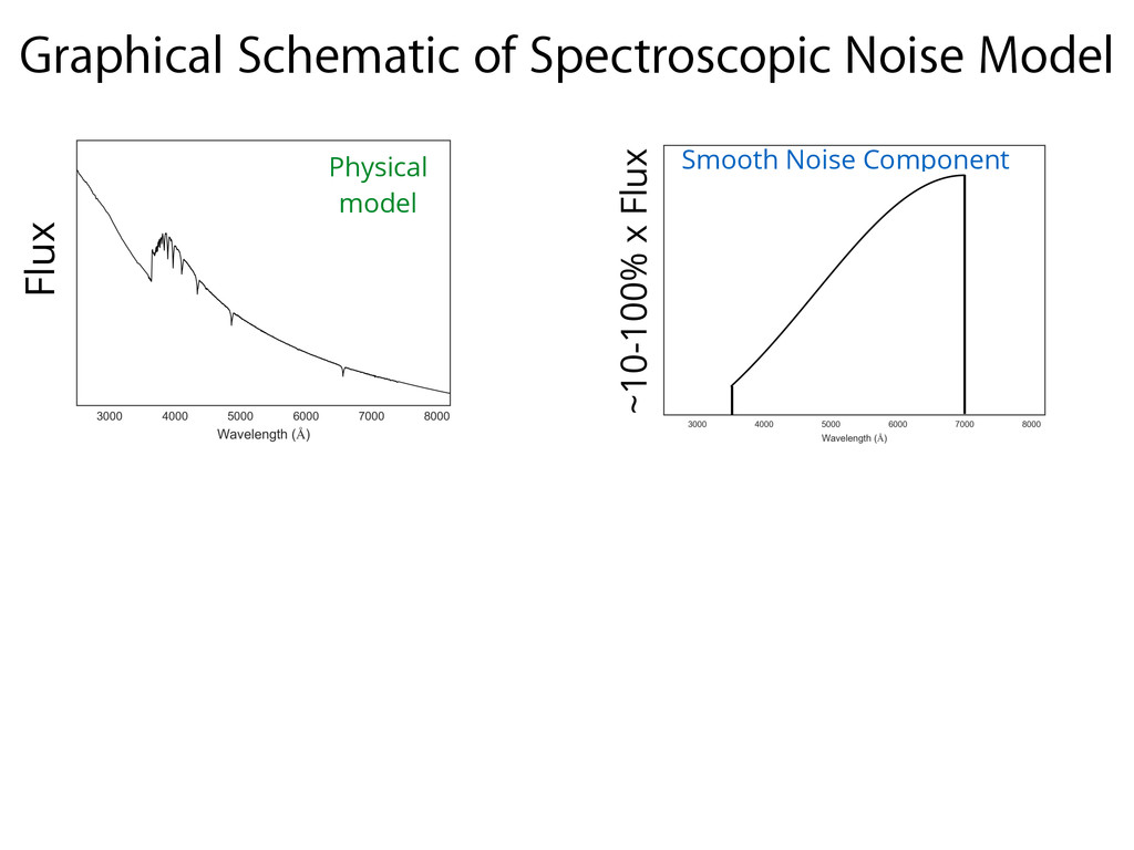
cal- alibration- to produce pect to the can be ex- However, gth ranges, calibration ynomials) It is there- odel of the n the like- lization of hat allows ntroduced dified log- ⇤ smaller `. The multiplication by µn µn0 in the kernel function signifies that it is defined in fractional terms. Using a high order polynomial can result in strong degeneracies between model and polynomial parameters, whereas the Gaussian Pro cess BDJ make this more precise and correct likelihood only reduces the penalty for residuals on the scale of ` with ampli tude a that can’t be fit by the mean model. The two log-likelihoods, for photometry and spectroscopy are combined into a single likelihood function, ln p(ds,dp |✓,↵,b) = ln pspec(ds |✓,↵)+ln pphot(dp |✓,b) . (10 where now ds is the spectroscopic data and dp is the photo metric data. The spectroscopic likelihood pspec is given by equation (3) and pphot is given by equation (2). 3. DATA AND EXPERIMENTAL SETUP We are now left to demonstrate that, by including photom etry as well as spectroscopy, it is possible to infer the param eters of interest ✓ while marginalizing over the calibration pa ds : spectroscopy dP : photometry
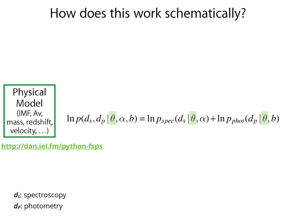
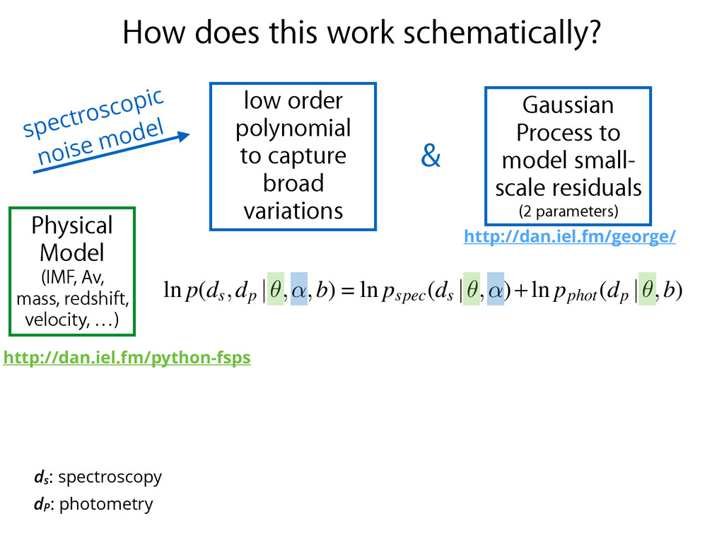
cal- alibration- to produce pect to the can be ex- However, gth ranges, calibration ynomials) It is there- odel of the n the like- lization of hat allows ntroduced dified log- ⇤ smaller `. The multiplication by µn µn0 in the kernel function signifies that it is defined in fractional terms. Using a high order polynomial can result in strong degeneracies between model and polynomial parameters, whereas the Gaussian Pro cess BDJ make this more precise and correct likelihood only reduces the penalty for residuals on the scale of ` with ampli tude a that can’t be fit by the mean model. The two log-likelihoods, for photometry and spectroscopy are combined into a single likelihood function, ln p(ds,dp |✓,↵,b) = ln pspec(ds |✓,↵)+ln pphot(dp |✓,b) . (10 where now ds is the spectroscopic data and dp is the photo metric data. The spectroscopic likelihood pspec is given by equation (3) and pphot is given by equation (2). 3. DATA AND EXPERIMENTAL SETUP We are now left to demonstrate that, by including photom etry as well as spectroscopy, it is possible to infer the param eters of interest ✓ while marginalizing over the calibration pa Physical Model (IMF, Av, mass, redshift, velocity, …) http://dan.iel.fm/python-fsps ds : spectroscopy dP : photometry
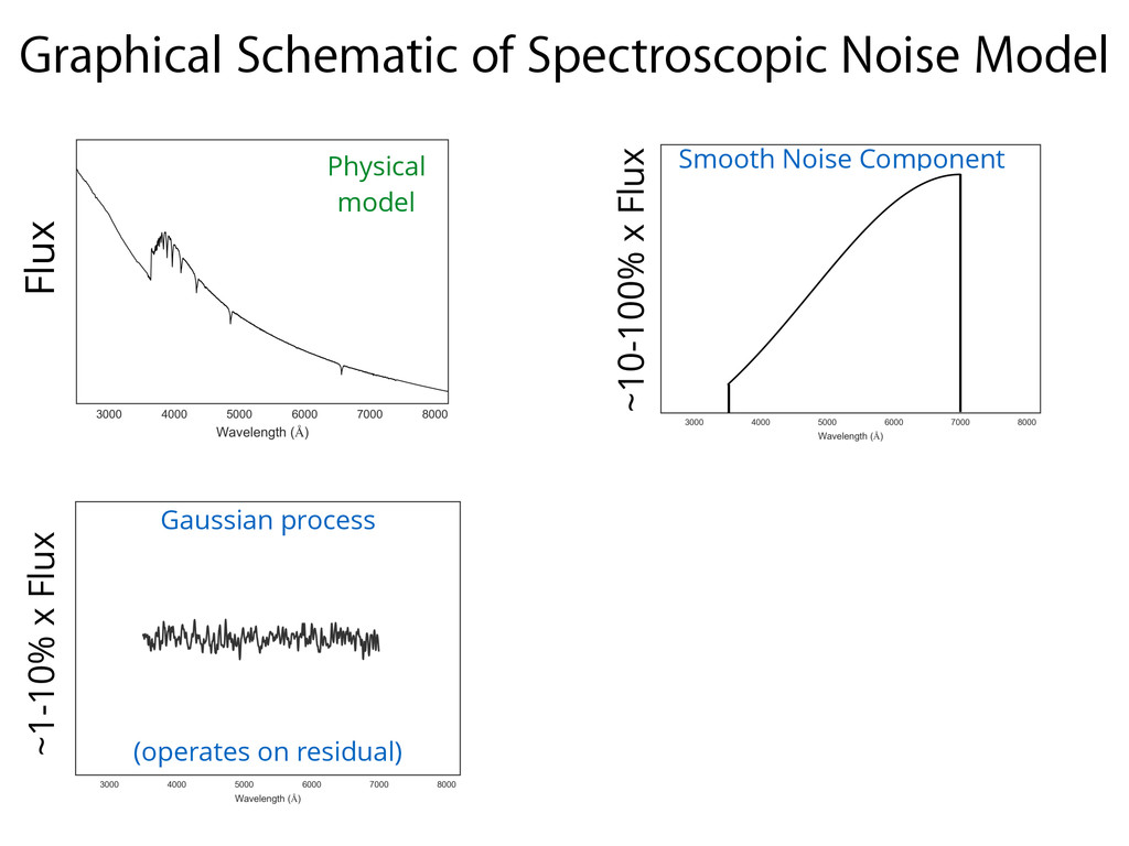
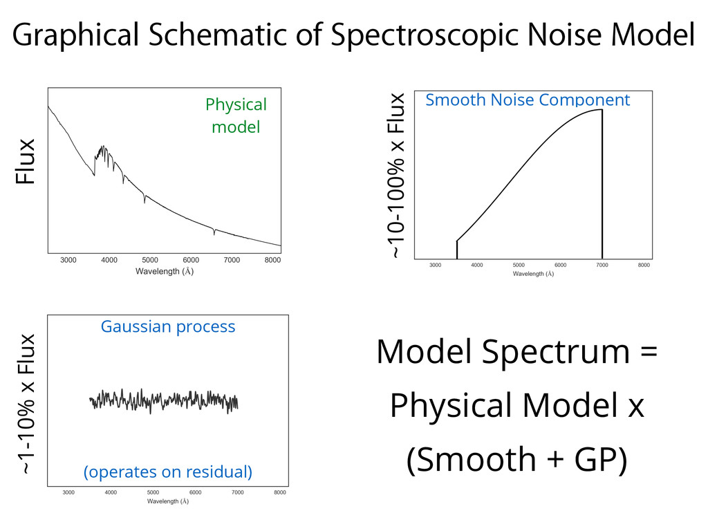
cal- alibration- to produce pect to the can be ex- However, gth ranges, calibration ynomials) It is there- odel of the n the like- lization of hat allows ntroduced dified log- ⇤ smaller `. The multiplication by µn µn0 in the kernel function signifies that it is defined in fractional terms. Using a high order polynomial can result in strong degeneracies between model and polynomial parameters, whereas the Gaussian Pro cess BDJ make this more precise and correct likelihood only reduces the penalty for residuals on the scale of ` with ampli tude a that can’t be fit by the mean model. The two log-likelihoods, for photometry and spectroscopy are combined into a single likelihood function, ln p(ds,dp |✓,↵,b) = ln pspec(ds |✓,↵)+ln pphot(dp |✓,b) . (10 where now ds is the spectroscopic data and dp is the photo metric data. The spectroscopic likelihood pspec is given by equation (3) and pphot is given by equation (2). 3. DATA AND EXPERIMENTAL SETUP We are now left to demonstrate that, by including photom etry as well as spectroscopy, it is possible to infer the param eters of interest ✓ while marginalizing over the calibration pa Physical Model (IMF, Av, mass, redshift, velocity, …) http://dan.iel.fm/python-fsps low order polynomial to capture broad variations spectroscopic noise model Gaussian Process to model small- scale residuals (2 parameters) & http://dan.iel.fm/george/ ds : spectroscopy dP : photometry
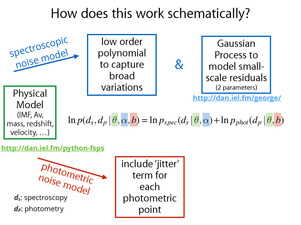
cal- alibration- to produce pect to the can be ex- However, gth ranges, calibration ynomials) It is there- odel of the n the like- lization of hat allows ntroduced dified log- ⇤ smaller `. The multiplication by µn µn0 in the kernel function signifies that it is defined in fractional terms. Using a high order polynomial can result in strong degeneracies between model and polynomial parameters, whereas the Gaussian Pro cess BDJ make this more precise and correct likelihood only reduces the penalty for residuals on the scale of ` with ampli tude a that can’t be fit by the mean model. The two log-likelihoods, for photometry and spectroscopy are combined into a single likelihood function, ln p(ds,dp |✓,↵,b) = ln pspec(ds |✓,↵)+ln pphot(dp |✓,b) . (10 where now ds is the spectroscopic data and dp is the photo metric data. The spectroscopic likelihood pspec is given by equation (3) and pphot is given by equation (2). 3. DATA AND EXPERIMENTAL SETUP We are now left to demonstrate that, by including photom etry as well as spectroscopy, it is possible to infer the param eters of interest ✓ while marginalizing over the calibration pa Physical Model (IMF, Av, mass, redshift, velocity, …) http://dan.iel.fm/python-fsps low order polynomial to capture broad variations spectroscopic noise model Gaussian Process to model small- scale residuals (2 parameters) & http://dan.iel.fm/george/ include ‘jitter’ term for each photometric point photometric noise model ds : spectroscopy dP : photometry
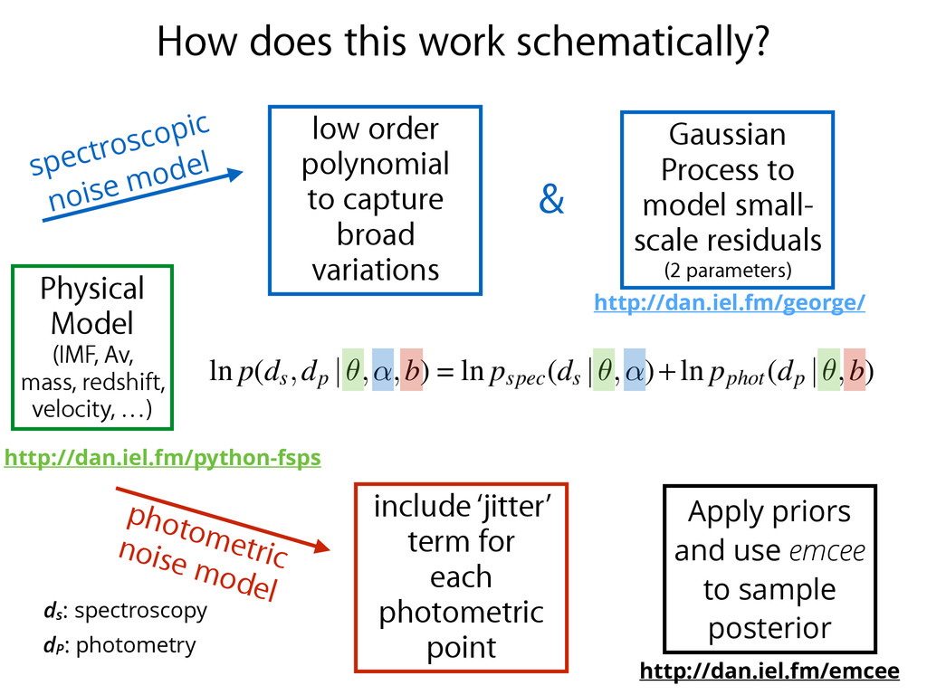
cal- alibration- to produce pect to the can be ex- However, gth ranges, calibration ynomials) It is there- odel of the n the like- lization of hat allows ntroduced dified log- ⇤ smaller `. The multiplication by µn µn0 in the kernel function signifies that it is defined in fractional terms. Using a high order polynomial can result in strong degeneracies between model and polynomial parameters, whereas the Gaussian Pro cess BDJ make this more precise and correct likelihood only reduces the penalty for residuals on the scale of ` with ampli tude a that can’t be fit by the mean model. The two log-likelihoods, for photometry and spectroscopy are combined into a single likelihood function, ln p(ds,dp |✓,↵,b) = ln pspec(ds |✓,↵)+ln pphot(dp |✓,b) . (10 where now ds is the spectroscopic data and dp is the photo metric data. The spectroscopic likelihood pspec is given by equation (3) and pphot is given by equation (2). 3. DATA AND EXPERIMENTAL SETUP We are now left to demonstrate that, by including photom etry as well as spectroscopy, it is possible to infer the param eters of interest ✓ while marginalizing over the calibration pa Physical Model (IMF, Av, mass, redshift, velocity, …) http://dan.iel.fm/python-fsps low order polynomial to capture broad variations spectroscopic noise model Gaussian Process to model small- scale residuals (2 parameters) & http://dan.iel.fm/george/ include ‘jitter’ term for each photometric point photometric noise model ds : spectroscopy dP : photometry Apply priors and use emcee to sample posterior http://dan.iel.fm/emcee
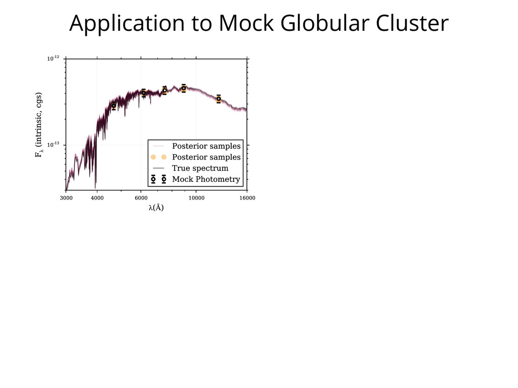
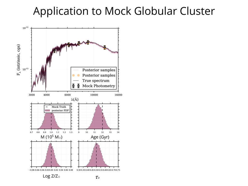
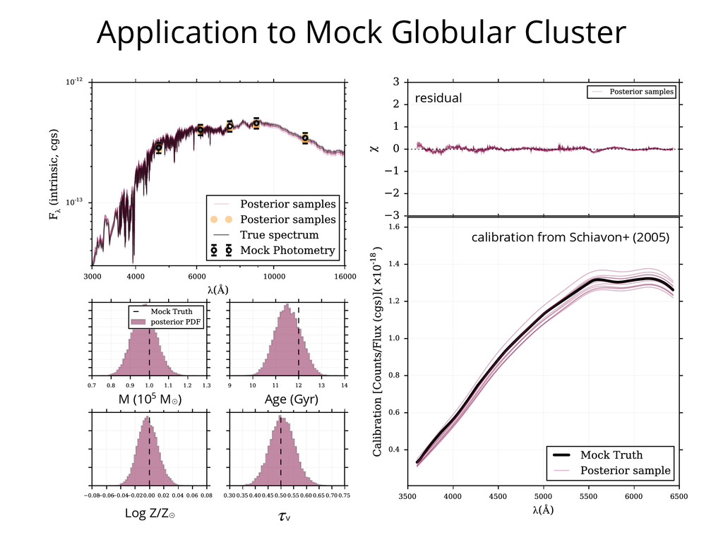
from the combination of uncalibrated spectroscopy and all the photometric data points. Panels and are as in Figure 2. residual Age (Gyr) Log Z/Z⊙ M (105 M⊙ ) v Application to Mock Globular Cluster calibration from Schiavon+ (2005)
from the combination of uncalibrated spectroscopy and all the photometric data points. Panels and are as in Figure 2. residual Age (Gyr) Log Z/Z⊙ M (105 M⊙ ) v Application to Mock Globular Cluster calibration from Schiavon+ (2005)
from the combination of uncalibrated spectroscopy and all the photometric data points. Panels and are as in Figure 2. residual Age (Gyr) Log Z/Z⊙ M (105 M⊙ ) v Application to Mock Globular Cluster calibration from Schiavon+ (2005)
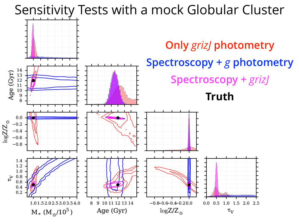
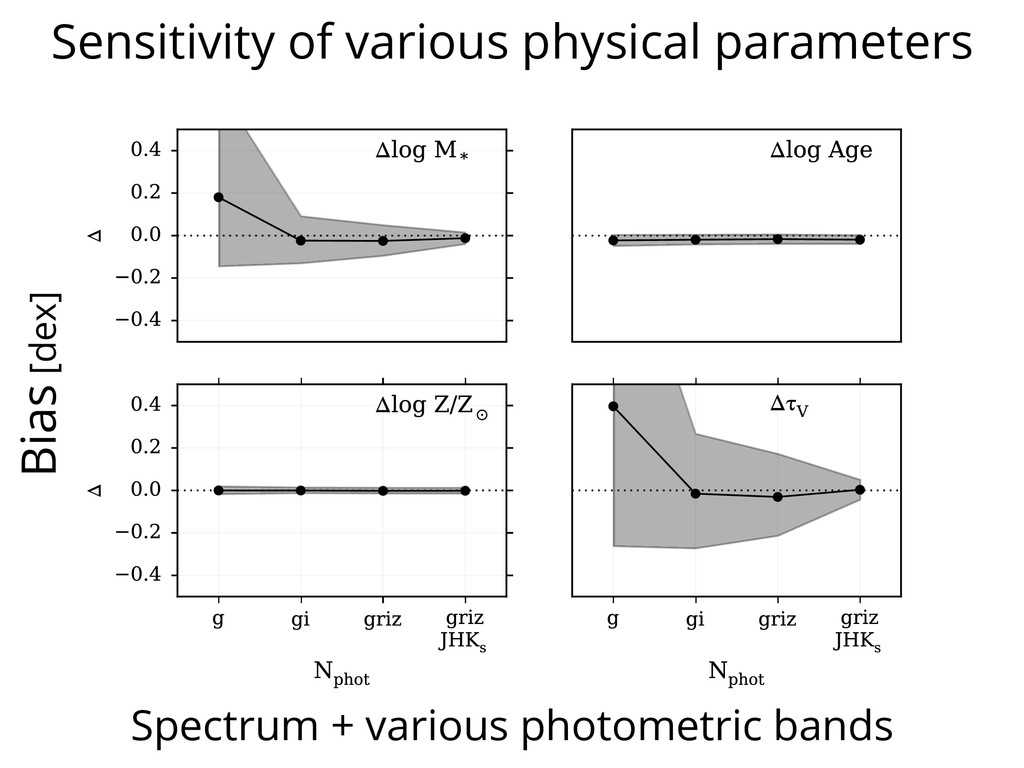
photometry in combination with optical spectroscopy. Marginalized posterior PDFs obtained from mock spectra and photometry, for different numbers of photometric bands. The medians of the posterior PDFs are shown as connected black circles, the 16th and 84th percentile of the posteriors are indicated by the gray shaded region. Sensitivity of various physical parameters Spectrum + various photometric bands Bias [dex]
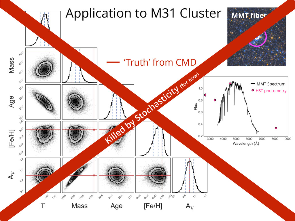
spectroscopic and photometric data together ‣ use all the available information; can be disjoint in wavelength ‣ no ad hoc weighting of data ‣ no need to subtract/normalize continuum ‣ physical parameters marginalized over data calibration ‣ learn about data/telescope calibration ‣ planned applications: stars, clusters, galaxies, … But not without some challenges… ‣ non-trivial to implement correctly ‣ modestly expensive to compute ‣ stochasticity http://dan.iel.fm/python-fsps http://dan.iel.fm/george/