The Local Group as a Time Machine

MPIA galaxy coffee on 2/4/2016

Transcript

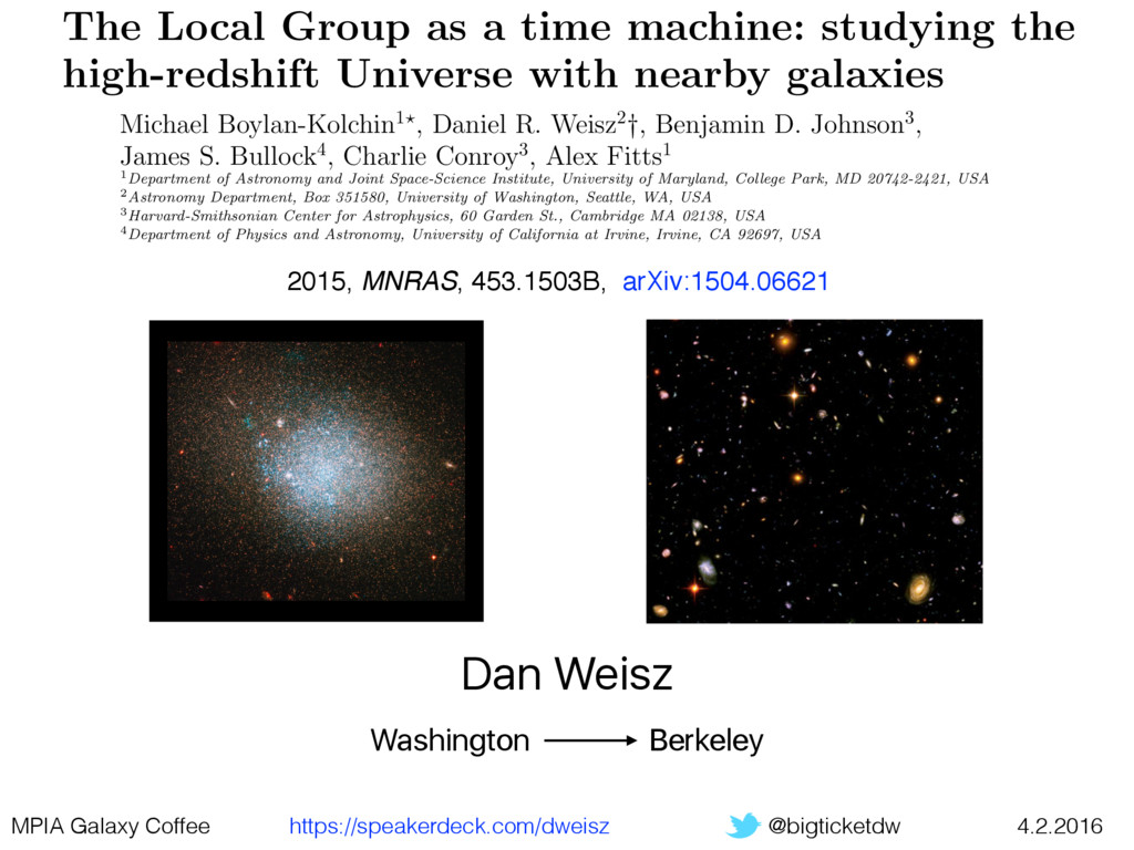
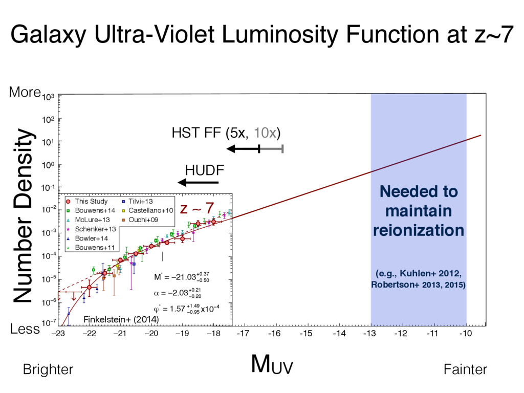
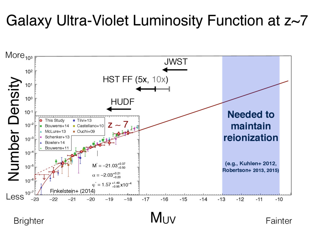
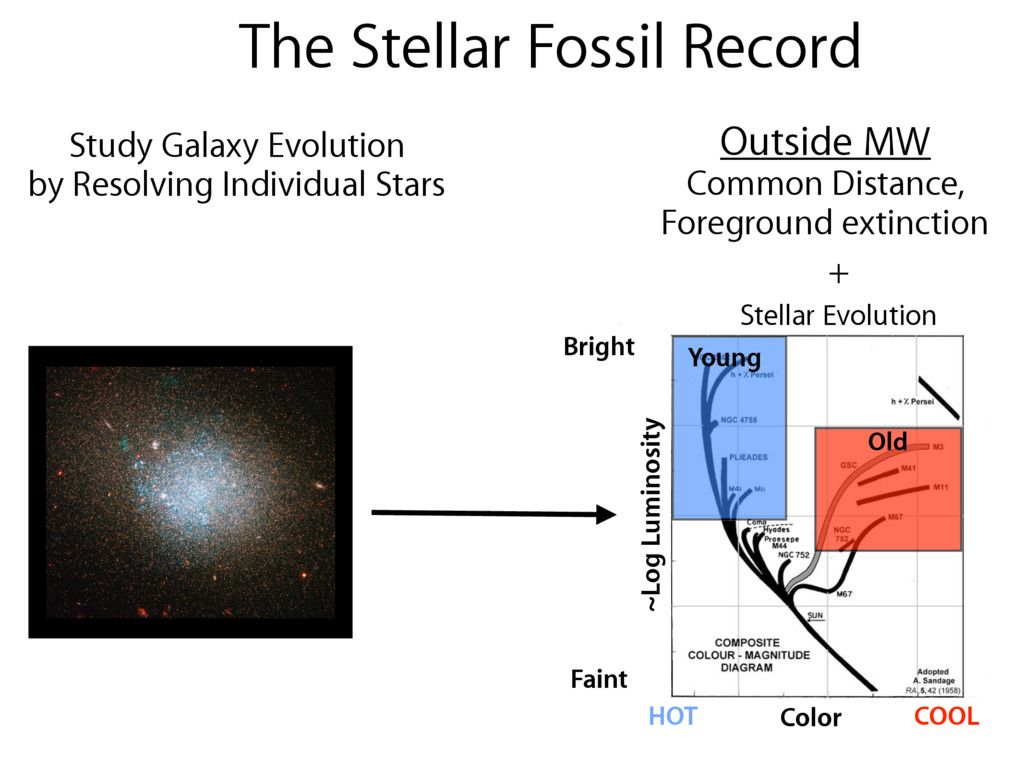
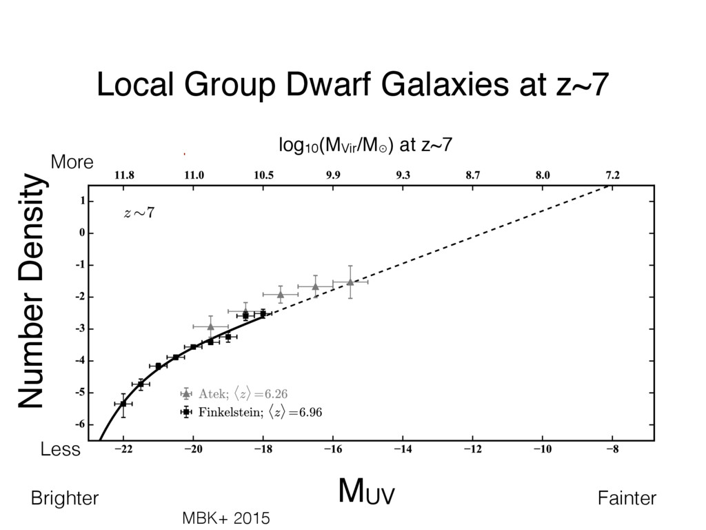
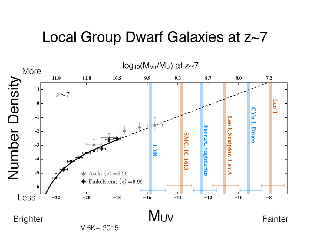
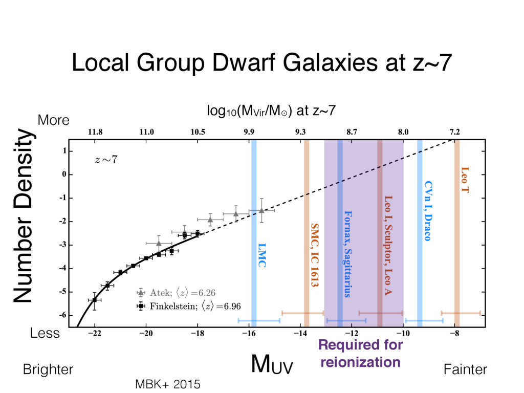
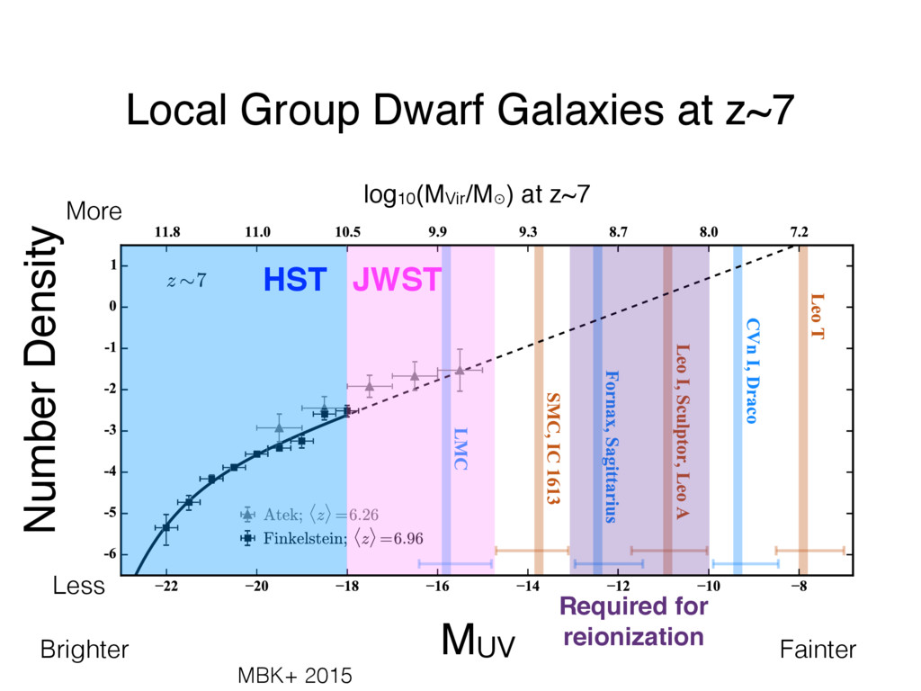
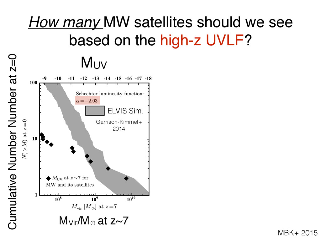
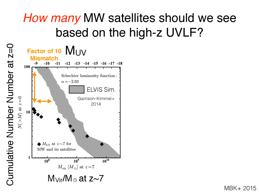
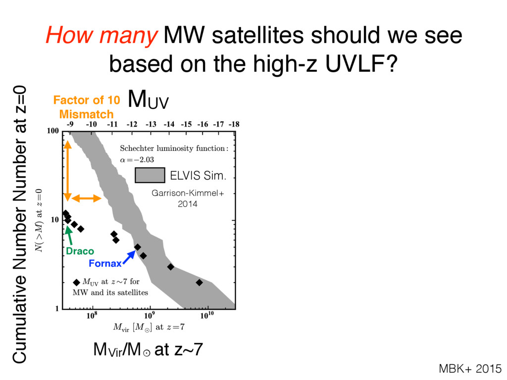
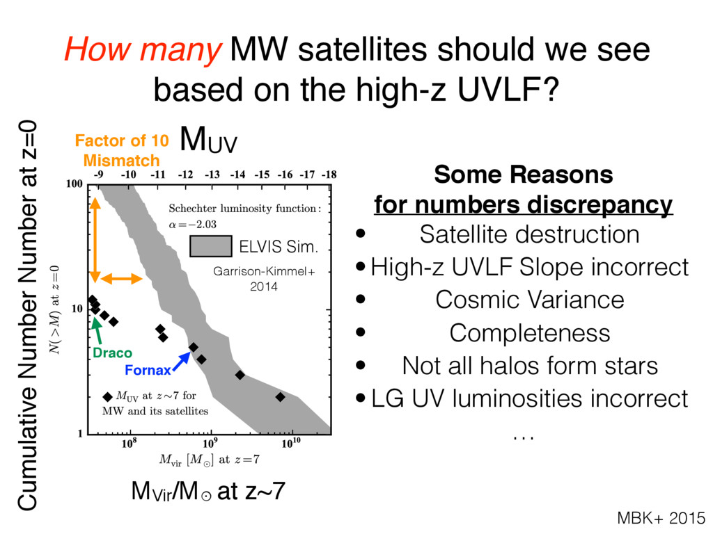
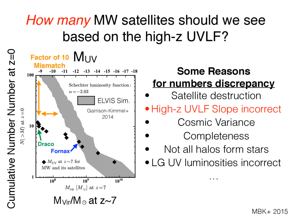
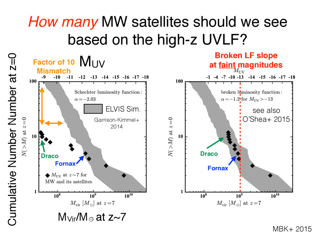
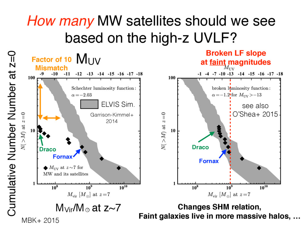
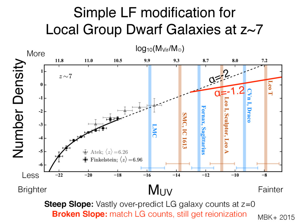
1. The Local Group as a time machine: studying the high-redshift Universe with nearby galaxies Michael Boylan-Kolchin 1? , Daniel R. Weisz 2† , Benjamin D. Johnson 3 , James S. Bullock 4 , Charlie Conroy 3 , Alex Fitts 1 1 Department of Astronomy and Joint Space-Science Institute, University of Maryland, College Park, MD 20742-2421, U 2 Astronomy Department, Box 351580, University of Washington, Seattle, WA, USA 3 Harvard-Smithsonian Center for Astrophysics, 60 Garden St., Cambridge MA 02138, USA 4 Department of Physics and Astronomy, University of California at Irvine, Irvine, CA 92697, USA 28 April 2015 ABSTRACT We infer the UV luminosities of Local Group galaxies at early cosmic t and z ⇠ 7) by combining stellar population synthesis modeling with sta histories derived from deep color-magnitude diagrams constructed from H Telescope (HST) observations. Our analysis provides a basis for understan galaxies – including those that may be unobservable even with the James Telescope (JWST) – in the context of familiar, well-studied objects in th Universe. We find that, at the epoch of reionization, all Local Group less luminous than the faintest galaxies detectable in deep HST observati fields. We predict that JWST will observe z ⇠ 7 progenitors of galaxie the Large Magellanic Cloud today; however, the HST Frontier Fields in already be observing such galaxies, highlighting the power of gravitatio Consensus reionization models require an extrapolation of the observed luminosity function at z ⇡ 7 by at least two orders of magnitude in order reionization. This scenario requires the progenitors of the Fornax and Sagit 1 [astro-ph.CO] 24 Apr 2015 The Local Group as a time machine: studying the high-redshift Universe with nearby galaxies Michael Boylan-Kolchin 1? , Daniel R. Weisz 2† , Benjamin D. Johnson 3 , James S. Bullock 4 , Charlie Conroy 3 , Alex Fitts 1 1 Department of Astronomy and Joint Space-Science Institute, University of Maryland, College Park, MD 20742-2421, USA 2 Astronomy Department, Box 351580, University of Washington, Seattle, WA, USA 3 Harvard-Smithsonian Center for Astrophysics, 60 Garden St., Cambridge MA 02138, USA 4 Department of Physics and Astronomy, University of California at Irvine, Irvine, CA 92697, USA 28 April 2015 ABSTRACT We infer the UV luminosities of Local Group galaxies at early cosmic times (z ⇠ 2 and z ⇠ 7) by combining stellar population synthesis modeling with star formation histories derived from deep color-magnitude diagrams constructed from Hubble Space Telescope (HST) observations. Our analysis provides a basis for understanding high-z galaxies – including those that may be unobservable even with the James Webb Space Telescope (JWST) – in the context of familiar, well-studied objects in the very low-z Universe. We find that, at the epoch of reionization, all Local Group dwarfs were less luminous than the faintest galaxies detectable in deep HST observations of blank fields. We predict that JWST will observe z ⇠ 7 progenitors of galaxies similar to the Large Magellanic Cloud today; however, the HST Frontier Fields initiative may already be observing such galaxies, highlighting the power of gravitational lensing. Consensus reionization models require an extrapolation of the observed blank-field luminosity function at z ⇡ 7 by at least two orders of magnitude in order to maintain reionization. This scenario requires the progenitors of the Fornax and Sagittarius dwarf spheroidal galaxies to be contributors to the ionizing background at z ⇠ 7. Combined with numerical simulations, our results argue for a break in the UV luminosity function from a faint-end slope of ↵ ⇠ 2 at MUV . 13 to ↵ ⇠ 1.2 at lower luminosities. Applied to photometric samples at lower redshifts, our analysis suggests that HST observations in lensing fields at z ⇠ 2 are capable of probing galaxies with luminosities comparable to the expected progenitor of Fornax. Key words: Local Group – galaxies: evolution – galaxies: high-redshift – cosmology: theory 504.06621v1 [astro-ph.CO] 24 Apr 2015 2015, MNRAS, 453.1503B, arXiv:1504.06621 Dan Weisz Washington Berkeley MPIA Galaxy Coffee 4.2.2016 https://speakerdeck.com/dweisz @bigticketdw
2. (z~6-10) A Primary Goal of high-z galaxy studies (HUDF, JWST, FF): Find, count, & characterize galaxies during reionization Current Consensus: Cosmic Reionization is powered by Galaxies
3. High-redshift observations State-of-the-art in deep fields (HST) CANDELS: The Rest-Frame UV Luminosity Function at z = 4–8 17 −21 −20 −19 −18 −17 lute UV Magnitude (1500 Å) z ∼ 4 y +14 urg+10 M* = −20.73+0.09 −0.09 α = −1.56+0.06 −0.05 ϕ* = 14.05 +2.05 −1.85 x10−4 −23 −22 −21 −20 −19 −18 −17 Absolute UV Magnitude (1500 Å) 10−7 10−6 10−5 10−4 10−3 10−2 ϕ (# Mag−1 Mpc−3) z ∼ 5 This Study Bouwens+14 van der Burg+10 McLure+09 M* = −20.81+0.13 −0.12 α = −1.67+0.05 −0.06 ϕ* = 8.95 +1.92 −1.31 x10−4 −21 −20 −19 −18 ute UV Magnitude (1500 Å) z ∼ 6 y 9 +07 +14 M* = −21.13+0.25 −0.31 α = −2.02+0.10 −0.10 ϕ* = 1.86 +0.94 −0.80 x10−4 −23 −22 −21 −20 −19 −18 Absolute UV Magnitude (1500 Å) 10−7 10−6 10−5 10−4 10−3 10−2 ϕ (# Mag−1 Mpc−3) z ∼ 7 This Study McLure+13 Schenker+13 Bowler+14 Bouwens+14 Bouwens+11 Tilvi+13 Castellano+10 Ouchi+09 M* = −21.03+0.37 −0.50 α = −2.03+0.21 −0.20 ϕ* = 1.57 +1.49 −0.95 x10−4 10−2 z ∼ 8 This Study Bouwens+14 Schmidt+14 Finkelstein et al. 2014 High-redshift observations State-of-the-art in deep fields (HST) CANDELS: The Rest-Frame UV Luminosity Function at z = 4–8 17 −23 −22 −21 −20 −19 −18 −17 Absolute UV Magnitude (1500 Å) 10−7 10−6 10−5 10−4 10−3 10−2 ϕ (# Mag−1 Mpc−3) z ∼ 4 This Study Bouwens+14 van der Burg+10 M* = −20.73+0.09 −0.09 α = −1.56+0.06 −0.05 ϕ* = 14.05 +2.05 −1.85 x10−4 −23 −22 −21 −20 −19 −18 −17 Absolute UV Magnitude (1500 Å) 10−7 10−6 10−5 10−4 10−3 10−2 ϕ (# Mag−1 Mpc−3) z ∼ 5 This Study Bouwens+14 van der Burg+10 McLure+09 M* = −20.81+0.13 −0.12 α = −1.67+0.05 −0.06 ϕ* = 8.95 +1.92 −1.31 x10−4 −23 −22 −21 −20 −19 −18 Absolute UV Magnitude (1500 Å) 10−7 10−6 10−5 10−4 10−3 10−2 ϕ (# Mag−1 Mpc−3) z ∼ 6 This Study McLure+09 Willott+13 Bouwens+07 Bouwens+14 M* = −21.13+0.25 −0.31 α = −2.02+0.10 −0.10 ϕ* = 1.86 +0.94 −0.80 x10−4 −23 −22 −21 −20 −19 −18 Absolute UV Magnitude (1500 Å) 10−7 10−6 10−5 10−4 10−3 10−2 ϕ (# Mag−1 Mpc−3) z ∼ 7 This Study McLure+13 Schenker+13 Bowler+14 Bouwens+14 Bouwens+11 Tilvi+13 Castellano+10 Ouchi+09 M* = −21.03+0.37 −0.50 α = −2.03+0.21 −0.20 ϕ* = 1.57 +1.49 −0.95 x10−4 10−2 z ∼ 8 This Study Bouwens+14 Schmidt+14 Finkelstein et al. 2 High-redshift observations State-of-the-art in deep fields (HST) −17 −23 −22 −21 −20 −19 −18 −17 Absolute UV Magnitude (1500 Å) 10−7 10−6 10−5 10−4 10−3 ϕ (# Mag−1 Mpc−3) McLure+09 M* = −20.81+0.13 −0.12 α = −1.67+0.05 −0.06 ϕ* = 8.95 +1.92 −1.31 x10−4 −23 −22 −21 −20 −19 −18 Absolute UV Magnitude (1500 Å) 10−7 10−6 10−5 10−4 10−3 10−2 ϕ (# Mag−1 Mpc−3) z ∼ 7 This Study McLure+13 Schenker+13 Bowler+14 Bouwens+14 Bouwens+11 Tilvi+13 Castellano+10 Ouchi+09 M* = −21.03+0.37 −0.50 α = −2.03+0.21 −0.20 ϕ* = 1.57 +1.49 −0.95 x10−4 z ∼ 8 13 4 1 M* = −20.89+0.74 −1.08 α = −2.36+0.54 −0.40 +2.52 Finkelstein et al. 2014 High-redshift observations State-of-the-art in deep fields (HST) −17 −23 −22 −21 −20 −19 −18 −17 Absolute UV Magnitude (1500 Å) 10−7 10−6 10−5 ϕ (# M* = −20.81+0.13 −0.12 α = −1.67+0.05 −0.06 ϕ* = 8.95 +1.92 −1.31 x10−4 −23 −22 −21 −20 −19 −18 Absolute UV Magnitude (1500 Å) 10−7 10−6 10−5 10−4 10−3 10−2 ϕ (# Mag−1 Mpc−3) z ∼ 7 This Study McLure+13 Schenker+13 Bowler+14 Bouwens+14 Bouwens+11 Tilvi+13 Castellano+10 Ouchi+09 M* = −21.03+0.37 −0.50 α = −2.03+0.21 −0.20 ϕ* = 1.57 +1.49 −0.95 x10−4 −21 −20 −19 −18 te UV Magnitude (1500 Å) z ∼ 8 13 4 1 M* = −20.89+0.74 −1.08 α = −2.36+0.54 −0.40 ϕ* = 0.72 +2.52 −0.65 x10−4 Finkelstein et al. 2014 me UV Luminosity Function at z = 4–8 17 −17 −23 −22 −21 −20 −19 −18 −17 Absolute UV Magnitude (1500 Å) 10−7 10−6 10−5 10−4 10−3 10−2 ϕ (# Mag−1 Mpc−3) z ∼ 5 This Study Bouwens+14 van der Burg+10 McLure+09 M* = −20.81+0.13 −0.12 α = −1.67+0.05 −0.06 ϕ* = 8.95 +1.92 −1.31 x10−4 −23 −22 −21 −20 −19 −18 Absolute UV Magnitude (1500 Å) 10−7 10−6 10−5 10−4 10−3 10−2 ϕ (# Mag−1 Mpc−3) z ∼ 7 This Study McLure+13 Schenker+13 Bowler+14 Bouwens+14 Bouwens+11 Tilvi+13 Castellano+10 Ouchi+09 M* = −21.03+0.37 −0.50 α = −2.03+0.21 −0.20 ϕ* = 1.57 +1.49 −0.95 x10−4 z ∼ 8 4 -17 -16 -15 -14 -13 -12 -11 -10 10-1 100 101 102 103 Number Density MUV Brighter Fainter Less More Galaxy Ultra-Violet Luminosity Function at z~7 Needed to maintain reionization (e.g., Kuhlen+ 2012, Robertson+ 2013, 2015) Finkelstein+ (2014)
4. High-redshift observations State-of-the-art in deep fields (HST) CANDELS: The Rest-Frame UV Luminosity Function at z = 4–8 17 −21 −20 −19 −18 −17 lute UV Magnitude (1500 Å) z ∼ 4 y +14 urg+10 M* = −20.73+0.09 −0.09 α = −1.56+0.06 −0.05 ϕ* = 14.05 +2.05 −1.85 x10−4 −23 −22 −21 −20 −19 −18 −17 Absolute UV Magnitude (1500 Å) 10−7 10−6 10−5 10−4 10−3 10−2 ϕ (# Mag−1 Mpc−3) z ∼ 5 This Study Bouwens+14 van der Burg+10 McLure+09 M* = −20.81+0.13 −0.12 α = −1.67+0.05 −0.06 ϕ* = 8.95 +1.92 −1.31 x10−4 −21 −20 −19 −18 ute UV Magnitude (1500 Å) z ∼ 6 y 9 +07 +14 M* = −21.13+0.25 −0.31 α = −2.02+0.10 −0.10 ϕ* = 1.86 +0.94 −0.80 x10−4 −23 −22 −21 −20 −19 −18 Absolute UV Magnitude (1500 Å) 10−7 10−6 10−5 10−4 10−3 10−2 ϕ (# Mag−1 Mpc−3) z ∼ 7 This Study McLure+13 Schenker+13 Bowler+14 Bouwens+14 Bouwens+11 Tilvi+13 Castellano+10 Ouchi+09 M* = −21.03+0.37 −0.50 α = −2.03+0.21 −0.20 ϕ* = 1.57 +1.49 −0.95 x10−4 10−2 z ∼ 8 This Study Bouwens+14 Schmidt+14 Finkelstein et al. 2014 High-redshift observations State-of-the-art in deep fields (HST) CANDELS: The Rest-Frame UV Luminosity Function at z = 4–8 17 −23 −22 −21 −20 −19 −18 −17 Absolute UV Magnitude (1500 Å) 10−7 10−6 10−5 10−4 10−3 10−2 ϕ (# Mag−1 Mpc−3) z ∼ 4 This Study Bouwens+14 van der Burg+10 M* = −20.73+0.09 −0.09 α = −1.56+0.06 −0.05 ϕ* = 14.05 +2.05 −1.85 x10−4 −23 −22 −21 −20 −19 −18 −17 Absolute UV Magnitude (1500 Å) 10−7 10−6 10−5 10−4 10−3 10−2 ϕ (# Mag−1 Mpc−3) z ∼ 5 This Study Bouwens+14 van der Burg+10 McLure+09 M* = −20.81+0.13 −0.12 α = −1.67+0.05 −0.06 ϕ* = 8.95 +1.92 −1.31 x10−4 −23 −22 −21 −20 −19 −18 Absolute UV Magnitude (1500 Å) 10−7 10−6 10−5 10−4 10−3 10−2 ϕ (# Mag−1 Mpc−3) z ∼ 6 This Study McLure+09 Willott+13 Bouwens+07 Bouwens+14 M* = −21.13+0.25 −0.31 α = −2.02+0.10 −0.10 ϕ* = 1.86 +0.94 −0.80 x10−4 −23 −22 −21 −20 −19 −18 Absolute UV Magnitude (1500 Å) 10−7 10−6 10−5 10−4 10−3 10−2 ϕ (# Mag−1 Mpc−3) z ∼ 7 This Study McLure+13 Schenker+13 Bowler+14 Bouwens+14 Bouwens+11 Tilvi+13 Castellano+10 Ouchi+09 M* = −21.03+0.37 −0.50 α = −2.03+0.21 −0.20 ϕ* = 1.57 +1.49 −0.95 x10−4 10−2 z ∼ 8 This Study Bouwens+14 Schmidt+14 Finkelstein et al. 2 High-redshift observations State-of-the-art in deep fields (HST) −17 −23 −22 −21 −20 −19 −18 −17 Absolute UV Magnitude (1500 Å) 10−7 10−6 10−5 10−4 10−3 ϕ (# Mag−1 Mpc−3) McLure+09 M* = −20.81+0.13 −0.12 α = −1.67+0.05 −0.06 ϕ* = 8.95 +1.92 −1.31 x10−4 −23 −22 −21 −20 −19 −18 Absolute UV Magnitude (1500 Å) 10−7 10−6 10−5 10−4 10−3 10−2 ϕ (# Mag−1 Mpc−3) z ∼ 7 This Study McLure+13 Schenker+13 Bowler+14 Bouwens+14 Bouwens+11 Tilvi+13 Castellano+10 Ouchi+09 M* = −21.03+0.37 −0.50 α = −2.03+0.21 −0.20 ϕ* = 1.57 +1.49 −0.95 x10−4 z ∼ 8 13 4 1 M* = −20.89+0.74 −1.08 α = −2.36+0.54 −0.40 +2.52 Finkelstein et al. 2014 High-redshift observations State-of-the-art in deep fields (HST) −17 −23 −22 −21 −20 −19 −18 −17 Absolute UV Magnitude (1500 Å) 10−7 10−6 10−5 ϕ (# M* = −20.81+0.13 −0.12 α = −1.67+0.05 −0.06 ϕ* = 8.95 +1.92 −1.31 x10−4 −23 −22 −21 −20 −19 −18 Absolute UV Magnitude (1500 Å) 10−7 10−6 10−5 10−4 10−3 10−2 ϕ (# Mag−1 Mpc−3) z ∼ 7 This Study McLure+13 Schenker+13 Bowler+14 Bouwens+14 Bouwens+11 Tilvi+13 Castellano+10 Ouchi+09 M* = −21.03+0.37 −0.50 α = −2.03+0.21 −0.20 ϕ* = 1.57 +1.49 −0.95 x10−4 −21 −20 −19 −18 te UV Magnitude (1500 Å) z ∼ 8 13 4 1 M* = −20.89+0.74 −1.08 α = −2.36+0.54 −0.40 ϕ* = 0.72 +2.52 −0.65 x10−4 Finkelstein et al. 2014 me UV Luminosity Function at z = 4–8 17 −17 −23 −22 −21 −20 −19 −18 −17 Absolute UV Magnitude (1500 Å) 10−7 10−6 10−5 10−4 10−3 10−2 ϕ (# Mag−1 Mpc−3) z ∼ 5 This Study Bouwens+14 van der Burg+10 McLure+09 M* = −20.81+0.13 −0.12 α = −1.67+0.05 −0.06 ϕ* = 8.95 +1.92 −1.31 x10−4 −23 −22 −21 −20 −19 −18 Absolute UV Magnitude (1500 Å) 10−7 10−6 10−5 10−4 10−3 10−2 ϕ (# Mag−1 Mpc−3) z ∼ 7 This Study McLure+13 Schenker+13 Bowler+14 Bouwens+14 Bouwens+11 Tilvi+13 Castellano+10 Ouchi+09 M* = −21.03+0.37 −0.50 α = −2.03+0.21 −0.20 ϕ* = 1.57 +1.49 −0.95 x10−4 z ∼ 8 4 -17 -16 -15 -14 -13 -12 -11 -10 10-1 100 101 102 103 Number Density MUV Brighter Fainter HUDF Less More Galaxy Ultra-Violet Luminosity Function at z~7 Needed to maintain reionization (e.g., Kuhlen+ 2012, Robertson+ 2013, 2015) Finkelstein+ (2014)
5. High-redshift observations State-of-the-art in deep fields (HST) CANDELS: The Rest-Frame UV Luminosity Function at z = 4–8 17 −21 −20 −19 −18 −17 lute UV Magnitude (1500 Å) z ∼ 4 y +14 urg+10 M* = −20.73+0.09 −0.09 α = −1.56+0.06 −0.05 ϕ* = 14.05 +2.05 −1.85 x10−4 −23 −22 −21 −20 −19 −18 −17 Absolute UV Magnitude (1500 Å) 10−7 10−6 10−5 10−4 10−3 10−2 ϕ (# Mag−1 Mpc−3) z ∼ 5 This Study Bouwens+14 van der Burg+10 McLure+09 M* = −20.81+0.13 −0.12 α = −1.67+0.05 −0.06 ϕ* = 8.95 +1.92 −1.31 x10−4 −21 −20 −19 −18 ute UV Magnitude (1500 Å) z ∼ 6 y 9 +07 +14 M* = −21.13+0.25 −0.31 α = −2.02+0.10 −0.10 ϕ* = 1.86 +0.94 −0.80 x10−4 −23 −22 −21 −20 −19 −18 Absolute UV Magnitude (1500 Å) 10−7 10−6 10−5 10−4 10−3 10−2 ϕ (# Mag−1 Mpc−3) z ∼ 7 This Study McLure+13 Schenker+13 Bowler+14 Bouwens+14 Bouwens+11 Tilvi+13 Castellano+10 Ouchi+09 M* = −21.03+0.37 −0.50 α = −2.03+0.21 −0.20 ϕ* = 1.57 +1.49 −0.95 x10−4 10−2 z ∼ 8 This Study Bouwens+14 Schmidt+14 Finkelstein et al. 2014 High-redshift observations State-of-the-art in deep fields (HST) CANDELS: The Rest-Frame UV Luminosity Function at z = 4–8 17 −23 −22 −21 −20 −19 −18 −17 Absolute UV Magnitude (1500 Å) 10−7 10−6 10−5 10−4 10−3 10−2 ϕ (# Mag−1 Mpc−3) z ∼ 4 This Study Bouwens+14 van der Burg+10 M* = −20.73+0.09 −0.09 α = −1.56+0.06 −0.05 ϕ* = 14.05 +2.05 −1.85 x10−4 −23 −22 −21 −20 −19 −18 −17 Absolute UV Magnitude (1500 Å) 10−7 10−6 10−5 10−4 10−3 10−2 ϕ (# Mag−1 Mpc−3) z ∼ 5 This Study Bouwens+14 van der Burg+10 McLure+09 M* = −20.81+0.13 −0.12 α = −1.67+0.05 −0.06 ϕ* = 8.95 +1.92 −1.31 x10−4 −23 −22 −21 −20 −19 −18 Absolute UV Magnitude (1500 Å) 10−7 10−6 10−5 10−4 10−3 10−2 ϕ (# Mag−1 Mpc−3) z ∼ 6 This Study McLure+09 Willott+13 Bouwens+07 Bouwens+14 M* = −21.13+0.25 −0.31 α = −2.02+0.10 −0.10 ϕ* = 1.86 +0.94 −0.80 x10−4 −23 −22 −21 −20 −19 −18 Absolute UV Magnitude (1500 Å) 10−7 10−6 10−5 10−4 10−3 10−2 ϕ (# Mag−1 Mpc−3) z ∼ 7 This Study McLure+13 Schenker+13 Bowler+14 Bouwens+14 Bouwens+11 Tilvi+13 Castellano+10 Ouchi+09 M* = −21.03+0.37 −0.50 α = −2.03+0.21 −0.20 ϕ* = 1.57 +1.49 −0.95 x10−4 10−2 z ∼ 8 This Study Bouwens+14 Schmidt+14 Finkelstein et al. 2 High-redshift observations State-of-the-art in deep fields (HST) −17 −23 −22 −21 −20 −19 −18 −17 Absolute UV Magnitude (1500 Å) 10−7 10−6 10−5 10−4 10−3 ϕ (# Mag−1 Mpc−3) McLure+09 M* = −20.81+0.13 −0.12 α = −1.67+0.05 −0.06 ϕ* = 8.95 +1.92 −1.31 x10−4 −23 −22 −21 −20 −19 −18 Absolute UV Magnitude (1500 Å) 10−7 10−6 10−5 10−4 10−3 10−2 ϕ (# Mag−1 Mpc−3) z ∼ 7 This Study McLure+13 Schenker+13 Bowler+14 Bouwens+14 Bouwens+11 Tilvi+13 Castellano+10 Ouchi+09 M* = −21.03+0.37 −0.50 α = −2.03+0.21 −0.20 ϕ* = 1.57 +1.49 −0.95 x10−4 z ∼ 8 13 4 1 M* = −20.89+0.74 −1.08 α = −2.36+0.54 −0.40 +2.52 Finkelstein et al. 2014 High-redshift observations State-of-the-art in deep fields (HST) −17 −23 −22 −21 −20 −19 −18 −17 Absolute UV Magnitude (1500 Å) 10−7 10−6 10−5 ϕ (# M* = −20.81+0.13 −0.12 α = −1.67+0.05 −0.06 ϕ* = 8.95 +1.92 −1.31 x10−4 −23 −22 −21 −20 −19 −18 Absolute UV Magnitude (1500 Å) 10−7 10−6 10−5 10−4 10−3 10−2 ϕ (# Mag−1 Mpc−3) z ∼ 7 This Study McLure+13 Schenker+13 Bowler+14 Bouwens+14 Bouwens+11 Tilvi+13 Castellano+10 Ouchi+09 M* = −21.03+0.37 −0.50 α = −2.03+0.21 −0.20 ϕ* = 1.57 +1.49 −0.95 x10−4 −21 −20 −19 −18 te UV Magnitude (1500 Å) z ∼ 8 13 4 1 M* = −20.89+0.74 −1.08 α = −2.36+0.54 −0.40 ϕ* = 0.72 +2.52 −0.65 x10−4 Finkelstein et al. 2014 me UV Luminosity Function at z = 4–8 17 −17 −23 −22 −21 −20 −19 −18 −17 Absolute UV Magnitude (1500 Å) 10−7 10−6 10−5 10−4 10−3 10−2 ϕ (# Mag−1 Mpc−3) z ∼ 5 This Study Bouwens+14 van der Burg+10 McLure+09 M* = −20.81+0.13 −0.12 α = −1.67+0.05 −0.06 ϕ* = 8.95 +1.92 −1.31 x10−4 −23 −22 −21 −20 −19 −18 Absolute UV Magnitude (1500 Å) 10−7 10−6 10−5 10−4 10−3 10−2 ϕ (# Mag−1 Mpc−3) z ∼ 7 This Study McLure+13 Schenker+13 Bowler+14 Bouwens+14 Bouwens+11 Tilvi+13 Castellano+10 Ouchi+09 M* = −21.03+0.37 −0.50 α = −2.03+0.21 −0.20 ϕ* = 1.57 +1.49 −0.95 x10−4 z ∼ 8 4 -17 -16 -15 -14 -13 -12 -11 -10 10-1 100 101 102 103 Number Density MUV Brighter Fainter HUDF HST FF (5x, 10x) Less More Galaxy Ultra-Violet Luminosity Function at z~7 Needed to maintain reionization (e.g., Kuhlen+ 2012, Robertson+ 2013, 2015) Finkelstein+ (2014)
6. High-redshift observations State-of-the-art in deep fields (HST) CANDELS: The Rest-Frame UV Luminosity Function at z = 4–8 17 −21 −20 −19 −18 −17 lute UV Magnitude (1500 Å) z ∼ 4 y +14 urg+10 M* = −20.73+0.09 −0.09 α = −1.56+0.06 −0.05 ϕ* = 14.05 +2.05 −1.85 x10−4 −23 −22 −21 −20 −19 −18 −17 Absolute UV Magnitude (1500 Å) 10−7 10−6 10−5 10−4 10−3 10−2 ϕ (# Mag−1 Mpc−3) z ∼ 5 This Study Bouwens+14 van der Burg+10 McLure+09 M* = −20.81+0.13 −0.12 α = −1.67+0.05 −0.06 ϕ* = 8.95 +1.92 −1.31 x10−4 −21 −20 −19 −18 ute UV Magnitude (1500 Å) z ∼ 6 y 9 +07 +14 M* = −21.13+0.25 −0.31 α = −2.02+0.10 −0.10 ϕ* = 1.86 +0.94 −0.80 x10−4 −23 −22 −21 −20 −19 −18 Absolute UV Magnitude (1500 Å) 10−7 10−6 10−5 10−4 10−3 10−2 ϕ (# Mag−1 Mpc−3) z ∼ 7 This Study McLure+13 Schenker+13 Bowler+14 Bouwens+14 Bouwens+11 Tilvi+13 Castellano+10 Ouchi+09 M* = −21.03+0.37 −0.50 α = −2.03+0.21 −0.20 ϕ* = 1.57 +1.49 −0.95 x10−4 10−2 z ∼ 8 This Study Bouwens+14 Schmidt+14 Finkelstein et al. 2014 High-redshift observations State-of-the-art in deep fields (HST) CANDELS: The Rest-Frame UV Luminosity Function at z = 4–8 17 −23 −22 −21 −20 −19 −18 −17 Absolute UV Magnitude (1500 Å) 10−7 10−6 10−5 10−4 10−3 10−2 ϕ (# Mag−1 Mpc−3) z ∼ 4 This Study Bouwens+14 van der Burg+10 M* = −20.73+0.09 −0.09 α = −1.56+0.06 −0.05 ϕ* = 14.05 +2.05 −1.85 x10−4 −23 −22 −21 −20 −19 −18 −17 Absolute UV Magnitude (1500 Å) 10−7 10−6 10−5 10−4 10−3 10−2 ϕ (# Mag−1 Mpc−3) z ∼ 5 This Study Bouwens+14 van der Burg+10 McLure+09 M* = −20.81+0.13 −0.12 α = −1.67+0.05 −0.06 ϕ* = 8.95 +1.92 −1.31 x10−4 −23 −22 −21 −20 −19 −18 Absolute UV Magnitude (1500 Å) 10−7 10−6 10−5 10−4 10−3 10−2 ϕ (# Mag−1 Mpc−3) z ∼ 6 This Study McLure+09 Willott+13 Bouwens+07 Bouwens+14 M* = −21.13+0.25 −0.31 α = −2.02+0.10 −0.10 ϕ* = 1.86 +0.94 −0.80 x10−4 −23 −22 −21 −20 −19 −18 Absolute UV Magnitude (1500 Å) 10−7 10−6 10−5 10−4 10−3 10−2 ϕ (# Mag−1 Mpc−3) z ∼ 7 This Study McLure+13 Schenker+13 Bowler+14 Bouwens+14 Bouwens+11 Tilvi+13 Castellano+10 Ouchi+09 M* = −21.03+0.37 −0.50 α = −2.03+0.21 −0.20 ϕ* = 1.57 +1.49 −0.95 x10−4 10−2 z ∼ 8 This Study Bouwens+14 Schmidt+14 Finkelstein et al. 2 High-redshift observations State-of-the-art in deep fields (HST) −17 −23 −22 −21 −20 −19 −18 −17 Absolute UV Magnitude (1500 Å) 10−7 10−6 10−5 10−4 10−3 ϕ (# Mag−1 Mpc−3) McLure+09 M* = −20.81+0.13 −0.12 α = −1.67+0.05 −0.06 ϕ* = 8.95 +1.92 −1.31 x10−4 −23 −22 −21 −20 −19 −18 Absolute UV Magnitude (1500 Å) 10−7 10−6 10−5 10−4 10−3 10−2 ϕ (# Mag−1 Mpc−3) z ∼ 7 This Study McLure+13 Schenker+13 Bowler+14 Bouwens+14 Bouwens+11 Tilvi+13 Castellano+10 Ouchi+09 M* = −21.03+0.37 −0.50 α = −2.03+0.21 −0.20 ϕ* = 1.57 +1.49 −0.95 x10−4 z ∼ 8 13 4 1 M* = −20.89+0.74 −1.08 α = −2.36+0.54 −0.40 +2.52 Finkelstein et al. 2014 High-redshift observations State-of-the-art in deep fields (HST) −17 −23 −22 −21 −20 −19 −18 −17 Absolute UV Magnitude (1500 Å) 10−7 10−6 10−5 ϕ (# M* = −20.81+0.13 −0.12 α = −1.67+0.05 −0.06 ϕ* = 8.95 +1.92 −1.31 x10−4 −23 −22 −21 −20 −19 −18 Absolute UV Magnitude (1500 Å) 10−7 10−6 10−5 10−4 10−3 10−2 ϕ (# Mag−1 Mpc−3) z ∼ 7 This Study McLure+13 Schenker+13 Bowler+14 Bouwens+14 Bouwens+11 Tilvi+13 Castellano+10 Ouchi+09 M* = −21.03+0.37 −0.50 α = −2.03+0.21 −0.20 ϕ* = 1.57 +1.49 −0.95 x10−4 −21 −20 −19 −18 te UV Magnitude (1500 Å) z ∼ 8 13 4 1 M* = −20.89+0.74 −1.08 α = −2.36+0.54 −0.40 ϕ* = 0.72 +2.52 −0.65 x10−4 Finkelstein et al. 2014 me UV Luminosity Function at z = 4–8 17 −17 −23 −22 −21 −20 −19 −18 −17 Absolute UV Magnitude (1500 Å) 10−7 10−6 10−5 10−4 10−3 10−2 ϕ (# Mag−1 Mpc−3) z ∼ 5 This Study Bouwens+14 van der Burg+10 McLure+09 M* = −20.81+0.13 −0.12 α = −1.67+0.05 −0.06 ϕ* = 8.95 +1.92 −1.31 x10−4 −23 −22 −21 −20 −19 −18 Absolute UV Magnitude (1500 Å) 10−7 10−6 10−5 10−4 10−3 10−2 ϕ (# Mag−1 Mpc−3) z ∼ 7 This Study McLure+13 Schenker+13 Bowler+14 Bouwens+14 Bouwens+11 Tilvi+13 Castellano+10 Ouchi+09 M* = −21.03+0.37 −0.50 α = −2.03+0.21 −0.20 ϕ* = 1.57 +1.49 −0.95 x10−4 z ∼ 8 4 -17 -16 -15 -14 -13 -12 -11 -10 10-1 100 101 102 103 Number Density MUV Brighter Fainter HUDF HST FF (5x, 10x) JWST Less More Galaxy Ultra-Violet Luminosity Function at z~7 Needed to maintain reionization (e.g., Kuhlen+ 2012, Robertson+ 2013, 2015) Finkelstein+ (2014)
7. Clever idea: Look for faint galaxies at epoch of reionization Problem: Faint galaxies are hard to observe! Another clever idea: Use the stellar fossil record of nearby dwarf galaxies to learn about reionization or where on the high-z UVLF do LG dwarf galaxies live?
8. Outside MW Common Distance, Foreground extinction Color ~Log Luminosity HOT COOL + Stellar Evolution Study Galaxy Evolution by Resolving Individual Stars The Stellar Fossil Record Bright Faint Young Old
9. Fornax LG dSph Example Star Formation History Weisz+ 2014a SFH from Fossil Record ➞ Ṃ(z)
10. Fornax LG dSph Example Star Formation History Reionization Challenge: stellar fossil record cannot resolve sub-Gyr SF events at high-z
11. Fluctuation amplitude & timescale matter! n the photometric redshift distribution of Finkelstein et al. and assuming that th a characteristic timescale of 20 Myr (left) or 200 Myr (right). The colors nel. In the case of 20 Myr bursts, the frequent and relatively high-amplitude n (with peaks corresponding to the burst and inter-burst periods). The 200 udes, result in a distribution that is less broad and is unimodal. This is a for 200 Myr bursts; the resulting SFH is therefore much closer to the fiducial z = 7 in each realization results in a cumulative distribution that is very Median=mode, 2 magnitude spread 4 M. Boylan-Kolchin et al. Figure 2. Probability distribution for M UV of Fornax, given the pho Fornax’s high-redshift star formation occurred in bursts with a char indicate the cumulative probability distribution in each panel. In th bursts result in a bimodal probability distribution function (with p Myr bursts, which are modeled with smaller burst amplitudes, res direct consequence of our smaller assumed burst amplitude for 200 M constant SFH. Taking the instantaneous value of M UV at z = 7 in similar to that shown here in each case. Median≠mode, 3 magnitude spread, bimodal distribution MBK et al. 2015 Effects of bursts on MUV (burst characteristics motivated by cosmological simulations) 200 Myr bursts 20 Myr bursts SFH from Fossil Record ➞ Ṃ(z) Ṃ(z) + Bursts + population synthesis ➞ MUV(z) Weisz+ 2012, 2014; MBK+2015
12. MV = -4.9 MV = -16.5 dSph dIrr dTrans dE ~104M⊙ ~109M⊙ Repeat exercise to get MUV at z~7 for many LG Dwarf Galaxies Weisz+ 2014a Plus newer data Cole+ 2007, 2014 Hidalgo+ 2011 Monelli+ 2010 Brown+ 2014 …
13. The Local Group in high-z context What did the progenitors of Local Group dwarfs look like at high redshift? How will galaxies that are observable with current and future observatories evolve to the present day? MBK, Weisz, et al. 2015 Number Density MUV Brighter Fainter Less More Local Group Dwarf Galaxies at z~7 log10(MVir/M⊙ ) at z~7 MBK+ 2015
14. The Local Group in high-z context What did the progenitors of Local Group dwarfs look like at high redshift? How will galaxies that are observable with current and future observatories evolve to the present day? MBK, Weisz, et al. 2015 Number Density MUV Brighter Fainter Less More Local Group Dwarf Galaxies at z~7 log10(MVir/M⊙ ) at z~7 MBK+ 2015
15. The Local Group in high-z context What did the progenitors of Local Group dwarfs look like at high redshift? How will galaxies that are observable with current and future observatories evolve to the present day? MBK, Weisz, et al. 2015 Number Density MUV Brighter Fainter Less More Required for reionization Local Group Dwarf Galaxies at z~7 log10(MVir/M⊙ ) at z~7 MBK+ 2015
16. The Local Group in high-z context What did the progenitors of Local Group dwarfs look like at high redshift? How will galaxies that are observable with current and future observatories evolve to the present day? MBK, Weisz, et al. 2015 Number Density MUV Brighter Fainter Less More Required for reionization HST JWST Local Group Dwarf Galaxies at z~7 log10(MVir/M⊙ ) at z~7 MBK+ 2015
17. 8 M. Boylan-Kolchin et al. Figure 5. The z = 7 mass function of the main progenitors of surviving z = 0 (sub)halos – including the main progenitor of the MW itself – within 300 kpc of the Milky Way based on the ELVIS simulations (shaded region). The upper horizontal axis gives the Figure 6. Similar to Figure 5, but assumes a UV luminosity function that breaks to ↵ = 1.2 at M UV > 13 (from the fiducial value of ↵ = 2.03 for brighter galaxies). The z = 7 census of galaxies surviving to z = 0 in the Milky Way is in How many MW satellites should we see based on the high-z UVLF? MVir/M⊙ at z~7 Cumulative Number Number at z=0 ELVIS Sim. Garrison-Kimmel+ 2014 MUV MBK+ 2015
18. 8 M. Boylan-Kolchin et al. Figure 5. The z = 7 mass function of the main progenitors of surviving z = 0 (sub)halos – including the main progenitor of the MW itself – within 300 kpc of the Milky Way based on the ELVIS simulations (shaded region). The upper horizontal axis gives the Figure 6. Similar to Figure 5, but assumes a UV luminosity function that breaks to ↵ = 1.2 at M UV > 13 (from the fiducial value of ↵ = 2.03 for brighter galaxies). The z = 7 census of galaxies surviving to z = 0 in the Milky Way is in How many MW satellites should we see based on the high-z UVLF? Cumulative Number Number at z=0 ELVIS Sim. Garrison-Kimmel+ 2014 Factor of 10 Mismatch MVir/M⊙ at z~7 MUV MBK+ 2015
19. 8 M. Boylan-Kolchin et al. Figure 5. The z = 7 mass function of the main progenitors of surviving z = 0 (sub)halos – including the main progenitor of the MW itself – within 300 kpc of the Milky Way based on the ELVIS simulations (shaded region). The upper horizontal axis gives the Figure 6. Similar to Figure 5, but assumes a UV luminosity function that breaks to ↵ = 1.2 at M UV > 13 (from the fiducial value of ↵ = 2.03 for brighter galaxies). The z = 7 census of galaxies surviving to z = 0 in the Milky Way is in How many MW satellites should we see based on the high-z UVLF? Cumulative Number Number at z=0 ELVIS Sim. Garrison-Kimmel+ 2014 Factor of 10 Mismatch Draco MVir/M⊙ at z~7 MUV MBK+ 2015 Fornax
20. 8 M. Boylan-Kolchin et al. Figure 5. The z = 7 mass function of the main progenitors of surviving z = 0 (sub)halos – including the main progenitor of the MW itself – within 300 kpc of the Milky Way based on the ELVIS simulations (shaded region). The upper horizontal axis gives the Figure 6. Similar to Figure 5, but assumes a UV luminosity function that breaks to ↵ = 1.2 at M UV > 13 (from the fiducial value of ↵ = 2.03 for brighter galaxies). The z = 7 census of galaxies surviving to z = 0 in the Milky Way is in How many MW satellites should we see based on the high-z UVLF? Cumulative Number Number at z=0 ELVIS Sim. Garrison-Kimmel+ 2014 Factor of 10 Mismatch Draco Some Reasons for numbers discrepancy • Satellite destruction •High-z UVLF Slope incorrect • Cosmic Variance • Completeness • Not all halos form stars • LG UV luminosities incorrect … MVir/M⊙ at z~7 MUV MBK+ 2015 Fornax
21. 8 M. Boylan-Kolchin et al. Figure 5. The z = 7 mass function of the main progenitors of surviving z = 0 (sub)halos – including the main progenitor of the MW itself – within 300 kpc of the Milky Way based on the ELVIS simulations (shaded region). The upper horizontal axis gives the Figure 6. Similar to Figure 5, but assumes a UV luminosity function that breaks to ↵ = 1.2 at M UV > 13 (from the fiducial value of ↵ = 2.03 for brighter galaxies). The z = 7 census of galaxies surviving to z = 0 in the Milky Way is in How many MW satellites should we see based on the high-z UVLF? Cumulative Number Number at z=0 ELVIS Sim. Garrison-Kimmel+ 2014 Factor of 10 Mismatch Draco Some Reasons for numbers discrepancy • Satellite destruction •High-z UVLF Slope incorrect • Cosmic Variance • Completeness • Not all halos form stars • LG UV luminosities incorrect … MVir/M⊙ at z~7 MUV MBK+ 2015 Fornax
22. 8 M. Boylan-Kolchin et al. Figure 5. The z = 7 mass function of the main progenitors of surviving z = 0 (sub)halos – including the main progenitor of the MW itself – within 300 kpc of the Milky Way based on the ELVIS simulations (shaded region). The upper horizontal axis gives the Figure 6. Similar to Figure 5, but assumes a UV luminosity function that breaks to ↵ = 1.2 at M UV > 13 (from the fiducial value of ↵ = 2.03 for brighter galaxies). The z = 7 census of galaxies surviving to z = 0 in the Milky Way is in How many MW satellites should we see based on the high-z UVLF? Cumulative Number Number at z=0 ELVIS Sim. Garrison-Kimmel+ 2014 Factor of 10 Mismatch Draco MVir/M⊙ at z~7 MUV Draco MBK+ 2015 see also O’Shea+ 2015 Broken LF slope at faint magnitudes Fornax Fornax
23. 8 M. Boylan-Kolchin et al. Figure 5. The z = 7 mass function of the main progenitors of surviving z = 0 (sub)halos – including the main progenitor of the MW itself – within 300 kpc of the Milky Way based on the ELVIS simulations (shaded region). The upper horizontal axis gives the Figure 6. Similar to Figure 5, but assumes a UV luminosity function that breaks to ↵ = 1.2 at M UV > 13 (from the fiducial value of ↵ = 2.03 for brighter galaxies). The z = 7 census of galaxies surviving to z = 0 in the Milky Way is in How many MW satellites should we see based on the high-z UVLF? Cumulative Number Number at z=0 ELVIS Sim. Garrison-Kimmel+ 2014 Factor of 10 Mismatch Draco Fornax MVir/M⊙ at z~7 MUV Draco Fornax Changes SHM relation, Faint galaxies live in more massive halos, … Broken LF slope at faint magnitudes see also O’Shea+ 2015 MBK+ 2015
24. The Local Group in high-z context What did the progenitors of Local Group dwarfs look like at high redshift? How will galaxies that are observable with current and future observatories evolve to the present day? MBK, Weisz, et al. 2015 Number Density Brighter Fainter Less More Simple LF modification for Local Group Dwarf Galaxies at z~7 log10(MVir/M⊙ ) α=-2 α=-1.2 Steep Slope: Vastly over-predict LG galaxy counts at z=0 Broken Slope: match LG counts, still get reionization MUV MBK+ 2015
25. Conclusions • There is a natural and fundamental connection between low- mass galaxies and cosmic reionization in all CDM models • Resolved stellar populations of nearby, faint galaxies may be the best pathway to study this connection • JWST unlikely to directly detect progenitors of Fornax at z~7 • Fossil Record for hundreds of low-mass galaxies within ~5 Mpc accessible with JWST • Improvements in stellar models & absolute stellar ages very important • Steep high-z UVLF slope over-predicts LG galaxy counts • Break in slope of -1.2 at MUV >-13 reconciles counts, maintains reionization • Better understanding of completeness in LG galaxy counts • Important to find more Draco to Fornax mass galaxies outside LG MBK, Weisz+ 2015 arXiv:1504.06621 Weisz+ 2014 arXiv:1409.4772 https://speakerdeck.com/dweisz MBK+ 2014 arXiv:1405.1040