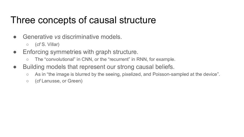
◦ (cf S. Villar) • Enforcing symmetries with graph structure. ◦ The “convolutional” in CNN, or the “recurrent” in RNN, for example. • Building models that represent our strong causal beliefs. ◦ As in “the image is blurred by the seeing, pixelized, and Poisson-sampled at the device”. ◦ (cf Lanusse, or Green)
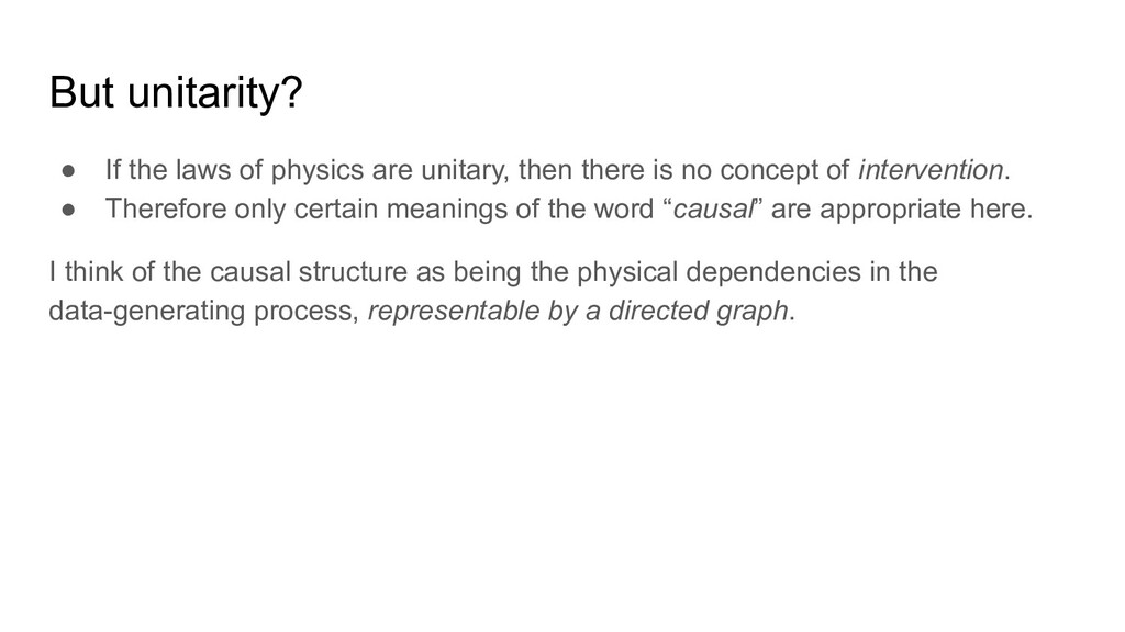
then there is no concept of intervention. • Therefore only certain meanings of the word “causal” are appropriate here. I think of the causal structure as being the physical dependencies in the data-generating process, representable by a directed graph.
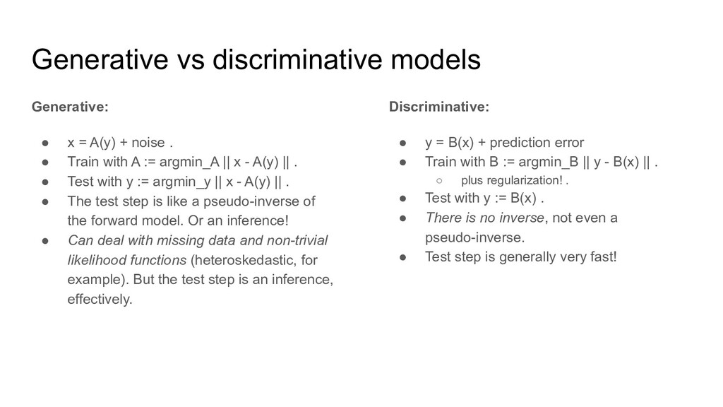
of your labels makes your data? ◦ x = A(y) ◦ Labels y generate the data x. • Or are you asking what function of your data makes your labels? ◦ y = B(x) ◦ Data x are transformed into labels y.
noise . • Train with A := argmin_A || x - A(y) || . • Test with y := argmin_y || x - A(y) || . • The test step is like a pseudo-inverse of the forward model. Or an inference! • Can deal with missing data and non-trivial likelihood functions (heteroskedastic, for example). But the test step is an inference, effectively. Discriminative: • y = B(x) + prediction error • Train with B := argmin_B || y - B(x) || . ◦ plus regularization! . • Test with y := B(x) . • There is no inverse, not even a pseudo-inverse. • Test step is generally very fast!
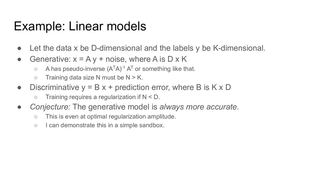
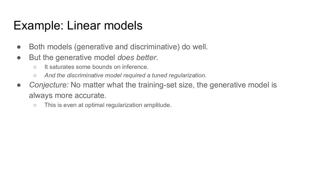
and the labels y be K-dimensional. • Generative: x = A y + noise, where A is D x K ◦ A has pseudo-inverse (ATA)-1 AT or something like that. ◦ Training data size N must be N > K. • Discriminative y = B x + prediction error, where B is K x D ◦ Training requires a regularization if N < D. • Conjecture: The generative model is always more accurate. ◦ This is even at optimal regularization amplitude. ◦ I can demonstrate this in a simple sandbox.
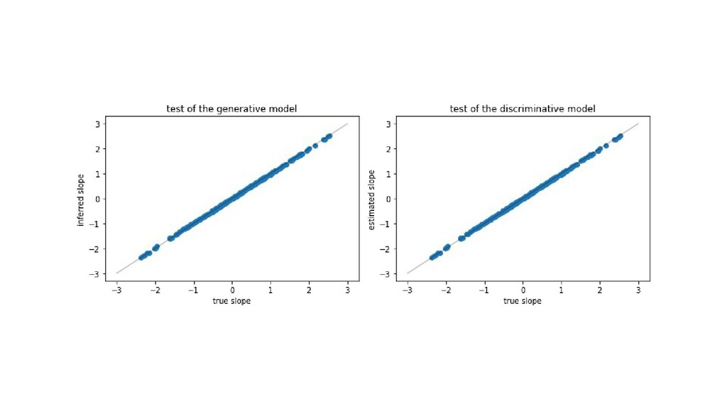
well. • But the generative model does better. ◦ It saturates some bounds on inference. ◦ And the discriminative model required a tuned regularization. • Conjecture: No matter what the training-set size, the generative model is always more accurate. ◦ This is even at optimal regularization amplitude.
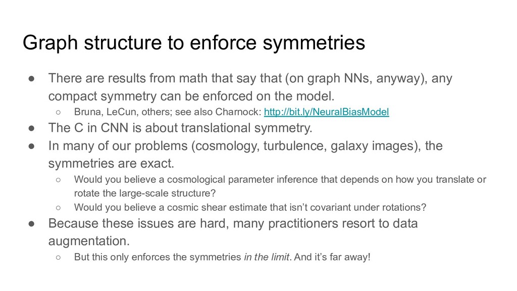
math that say that (on graph NNs, anyway), any compact symmetry can be enforced on the model. ◦ Bruna, LeCun, others; see also Charnock: http://bit.ly/NeuralBiasModel • The C in CNN is about translational symmetry. • In many of our problems (cosmology, turbulence, galaxy images), the symmetries are exact. ◦ Would you believe a cosmological parameter inference that depends on how you translate or rotate the large-scale structure? ◦ Would you believe a cosmic shear estimate that isn’t covariant under rotations? • Because these issues are hard, many practitioners resort to data augmentation. ◦ But this only enforces the symmetries in the limit. And it’s far away!
depends on Teff, log g, and element abundances. • The color of the star depends on its temperature and interstellar reddening, which in turn depends on its location in the Galaxy. • The galaxy image is sheared by the cosmological gravitational field, blurred by the Earth’s atmosphere, and pixelized by the detector.
stellar Doppler shifts at the m/s level. • Even at resolving power 100,000, this is 1/1000 of a pixel in the spectrograph. • Used to find or confirm many hundreds of extra-solar planets. ◦ And thousands more coming very soon. • Measured RVs are limited by our ability to model the atmosphere and star. ◦ (Not everyone would agree with this statement, but it’s a hill I’ll die on.) • The total signal-to-noise in typical data sets is immense. ◦ 100s of 100,000-pixel observations over many years with SNR of 100s each. • It was awarded the 2019 Nobel Prize. ◦ Mayor and Queloz
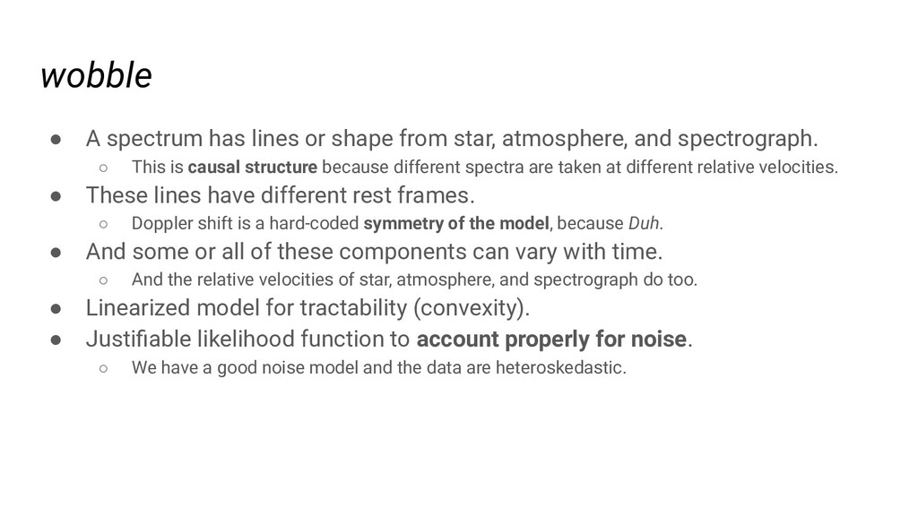
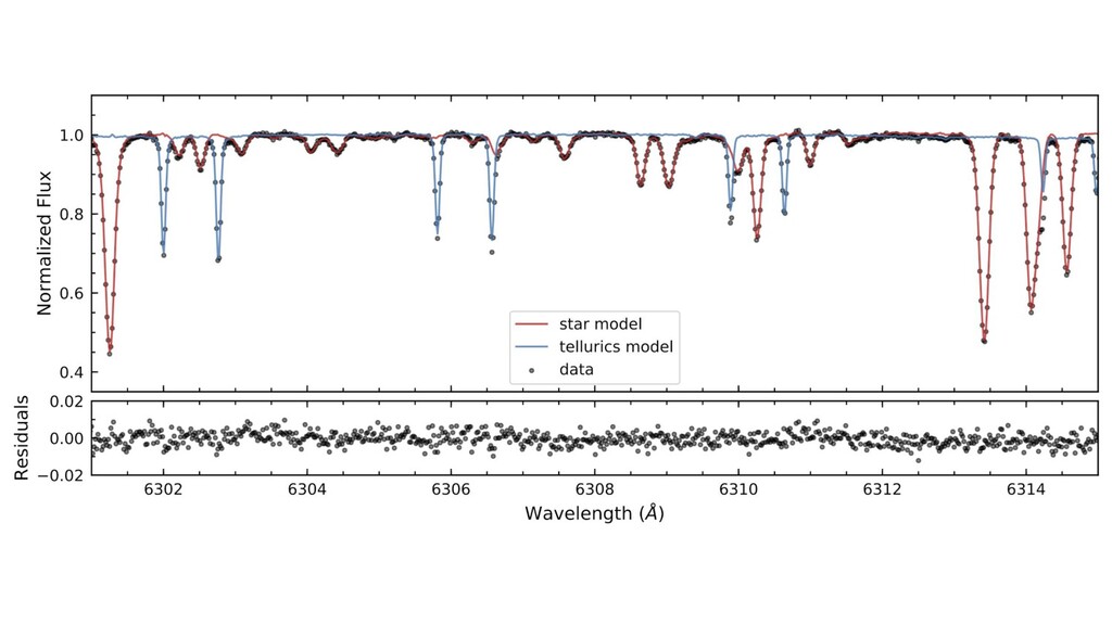
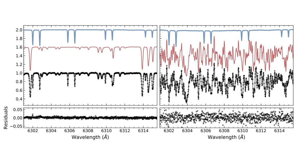
atmosphere, and spectrograph. ◦ This is causal structure because different spectra are taken at different relative velocities. • These lines have different rest frames. ◦ Doppler shift is a hard-coded symmetry of the model, because Duh. • And some or all of these components can vary with time. ◦ And the relative velocities of star, atmosphere, and spectrograph do too. • Linearized model for tractability (convexity). • Justifiable likelihood function to account properly for noise. ◦ We have a good noise model and the data are heteroskedastic.
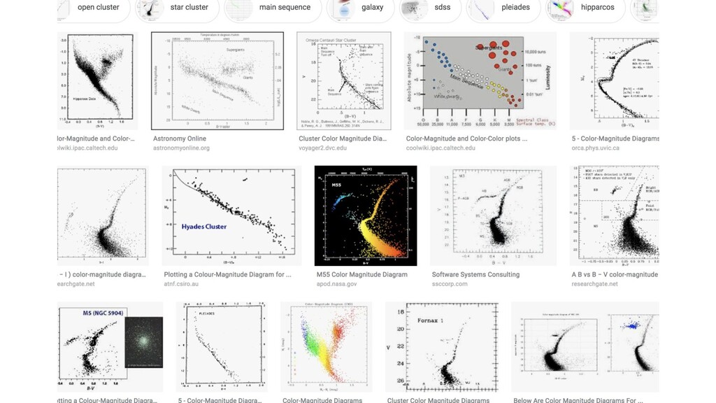
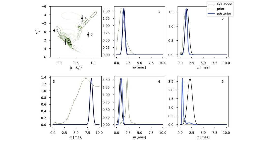
and temperature, stars lie in an amazingly structured and simple distribution. ◦ See, eg, the last 150 years of astronomy. ◦ Main sequence, red-giant branch, white dwarfs, horizontal branch, red clump, binary sequences, and so on. ◦ Almost one-dimensional! (with thickness) • Theory does a great job! But small, systematic deviations. ◦ These lead to biases if you want to use the theory to measure stellar properties, for example. • If we can understand the CMD well, we can infer distances to all the stars! • Gaia changed the world. ◦ Data now “outweigh” theory in many respects.
Widmark (Stockholm), Keith Hawkins (Texas), and others. • ESA Gaia DR1 data ◦ This is out of date now, of course. • arXiv:1706.05055, arXiv:1705.08988, arXiv:1703.08112
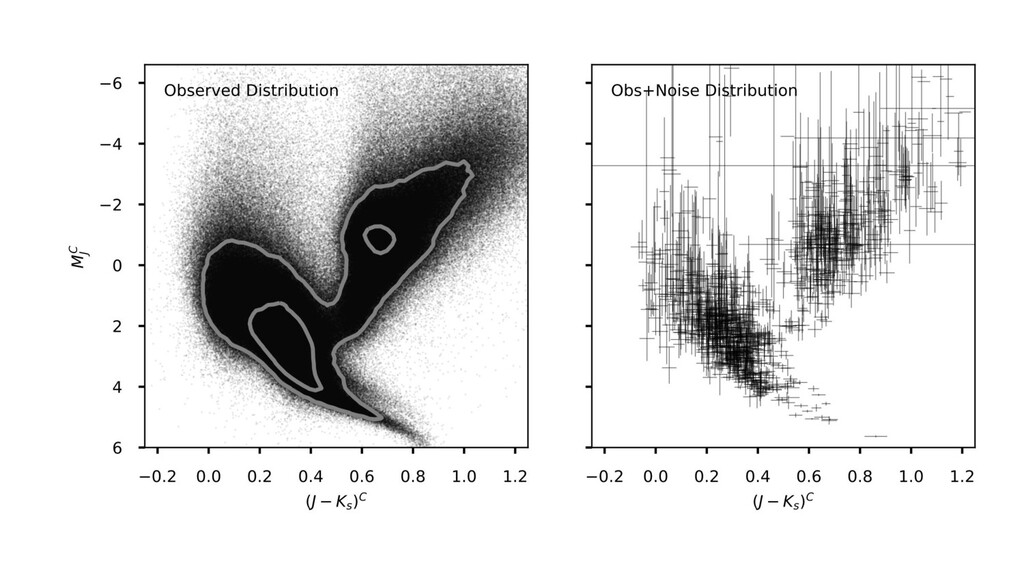
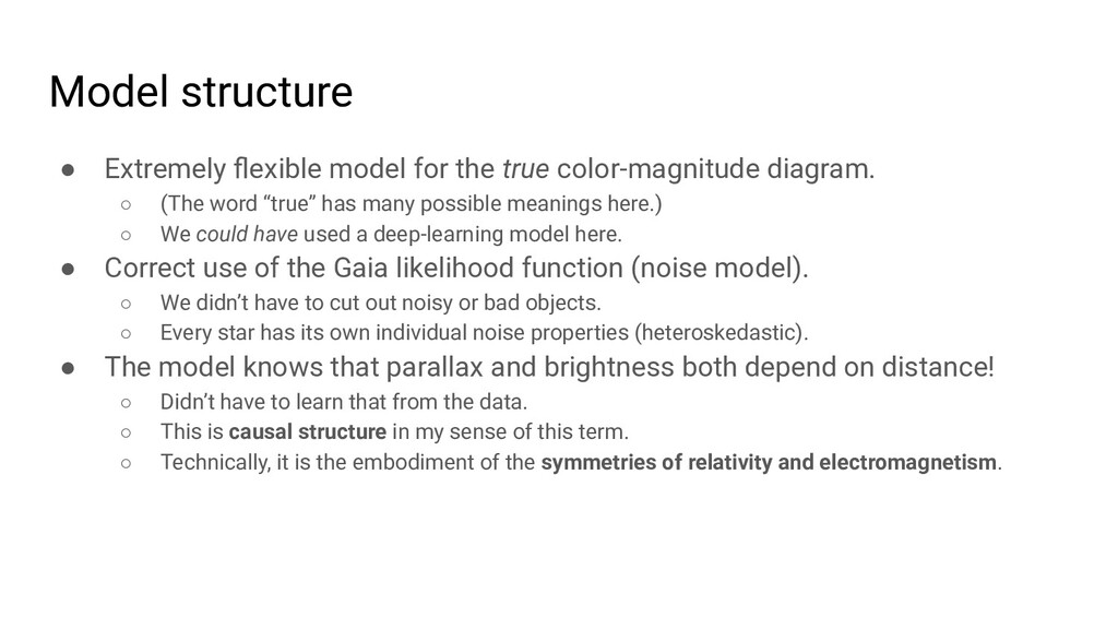
diagram. ◦ (The word “true” has many possible meanings here.) ◦ We could have used a deep-learning model here. • Correct use of the Gaia likelihood function (noise model). ◦ We didn’t have to cut out noisy or bad objects. ◦ Every star has its own individual noise properties (heteroskedastic). • The model knows that parallax and brightness both depend on distance! ◦ Didn’t have to learn that from the data. ◦ This is causal structure in my sense of this term. ◦ Technically, it is the embodiment of the symmetries of relativity and electromagnetism.
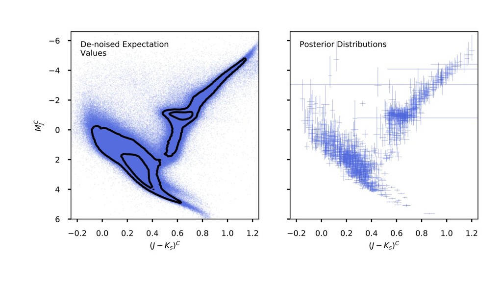
the Gaia data but produced more precise results than the Gaia data. What gives? • Stationarity assumption. ◦ Stars are similar to one another; related to statistical shrinkage. • Use of high-quality noise model. • Enforcing physical symmetries. ◦ Lorentz invariance (the symmetries of electromagnetism and spacetime). ◦ (But no other use of physical models of stars, which we don’t fully believe.) ◦ There is much more we could do!
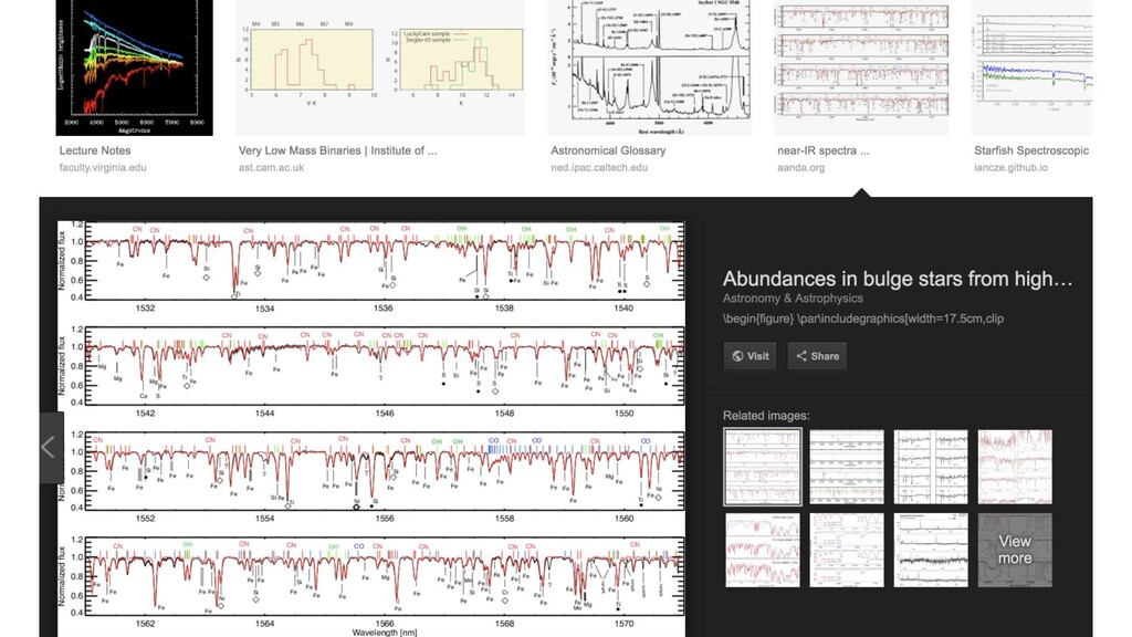
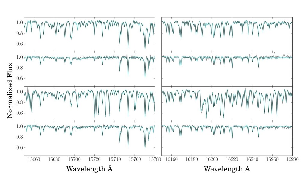
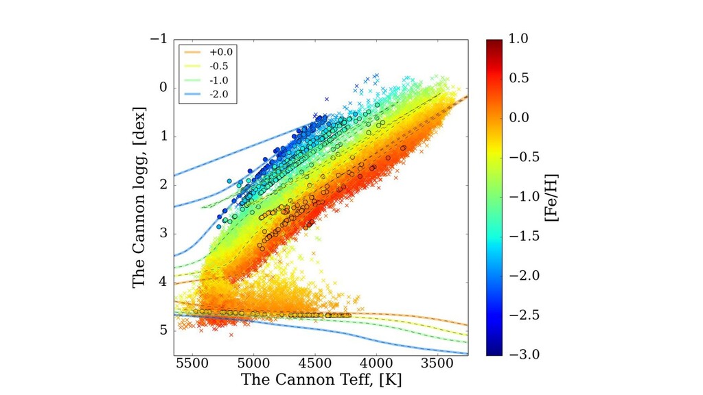
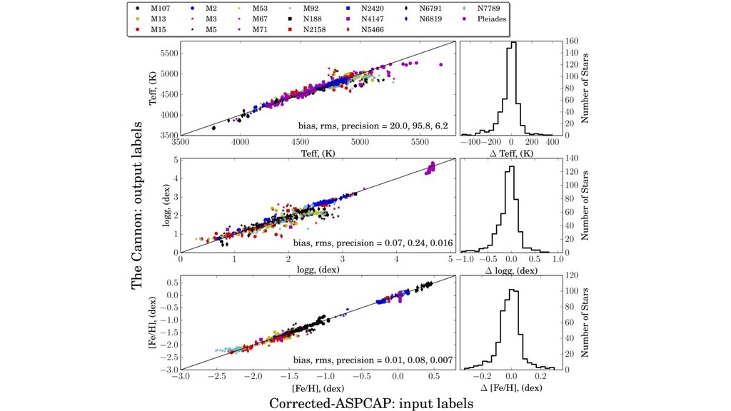
first-order parameters. ◦ Effective temperature, surface gravity, surface abundances (a few dominate). • These parameters reveal themselves in absorption-line strengths. • Stellar interior models and atmosphere models are amazingly detailed. ◦ Models predict spectra at the few-percent level or even better, depending on stuhh. ◦ And yet, the data are so incredible that we can see their failures at immense significance. • Spectroscopy at resolving power 20,000 to 100,000 is the standard tool. ◦ (wavelength over delta-wavelength)
Casey (Monash), Jessica Birky (UW), Hans-Walter Rix (MPIA), Soledad Villar (NYU), and many others. • SDSS-III and SDSS-IV APOGEE spectroscopy data. ◦ These are remarkable projects of which I am very fortunate to be a part. ◦ We have also run on other kinds of data from other projects. • arXiv:1501.07604, arXiv:1603.03040, arXiv:1609.03195, arXiv:1609.02914, arXiv:1602.00303, arXiv:1511.08204 … * It’s named after the person, not the weapon!
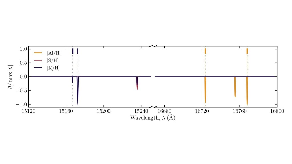
labels, from somewhere! ◦ I’m going to call parameters “labels”. • Every spectral pixel brightness (expectation) is a simple function of labels. • Righteous likelihood function for the spectral pixel brightnesses. ◦ Fully heteroskedastic. ◦ Can deal with missing data and low SNR spectra. • Model training is maximum-likelihood. • Model execution on new data is also maximum-likelihood.
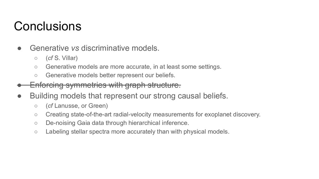
◦ Generative models are more accurate, in at least some settings. ◦ Generative models better represent our beliefs. • Enforcing symmetries with graph structure. • Building models that represent our strong causal beliefs. ◦ (cf Lanusse, or Green) ◦ Creating state-of-the-art radial-velocity measurements for exoplanet discovery. ◦ De-noising Gaia data through hierarchical inference. ◦ Labeling stellar spectra more accurately than with physical models.