that is purpose built for developing models using orthogonal polynomials. These models can be fit directly to real-world sensor data, simulation data, or even to other surrogate models. As you will discover, using orthogonal polynomials is very advantageous and can tell us a lot about the underlying data we are modelling. A FEW WORDS
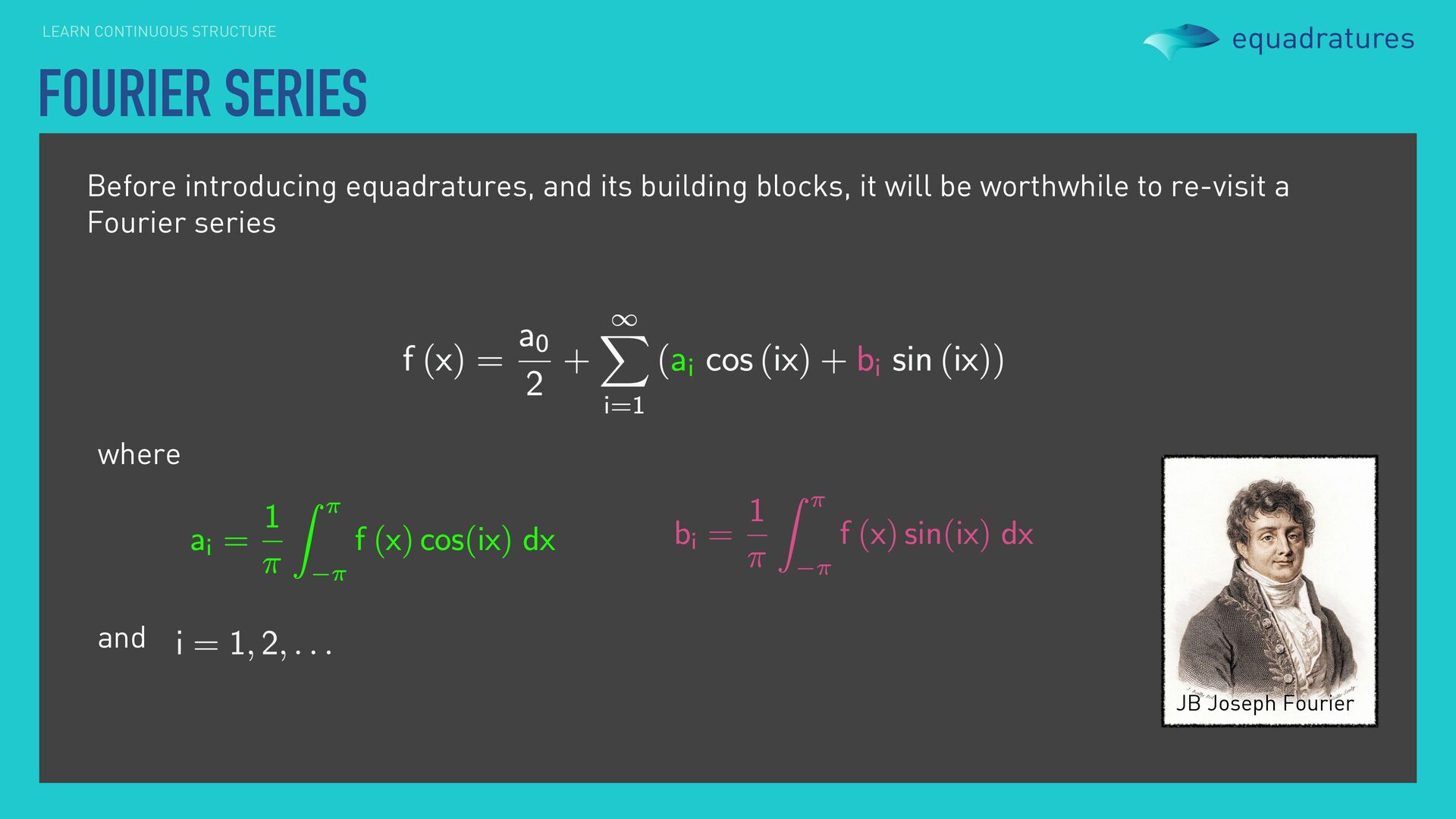
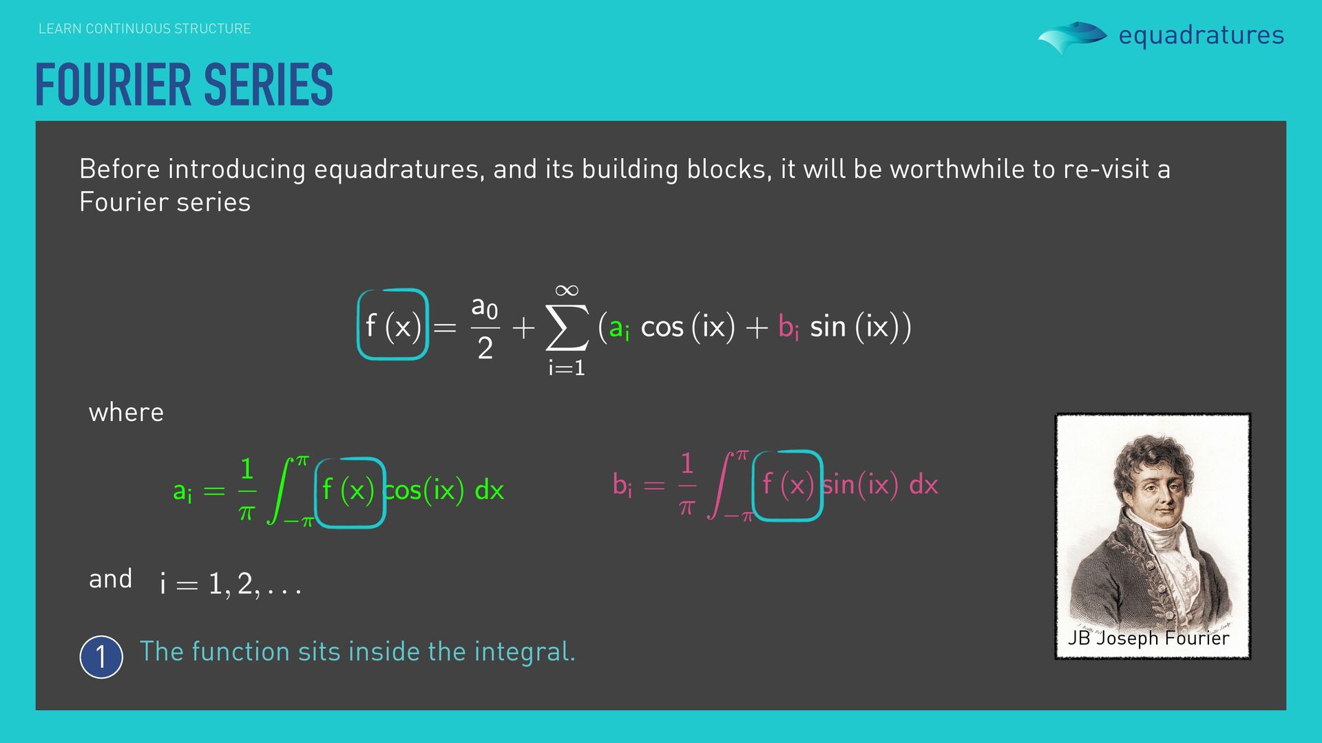
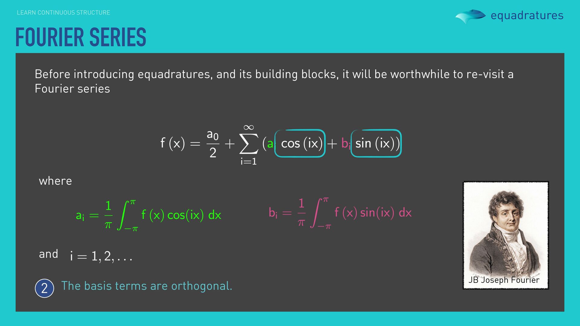
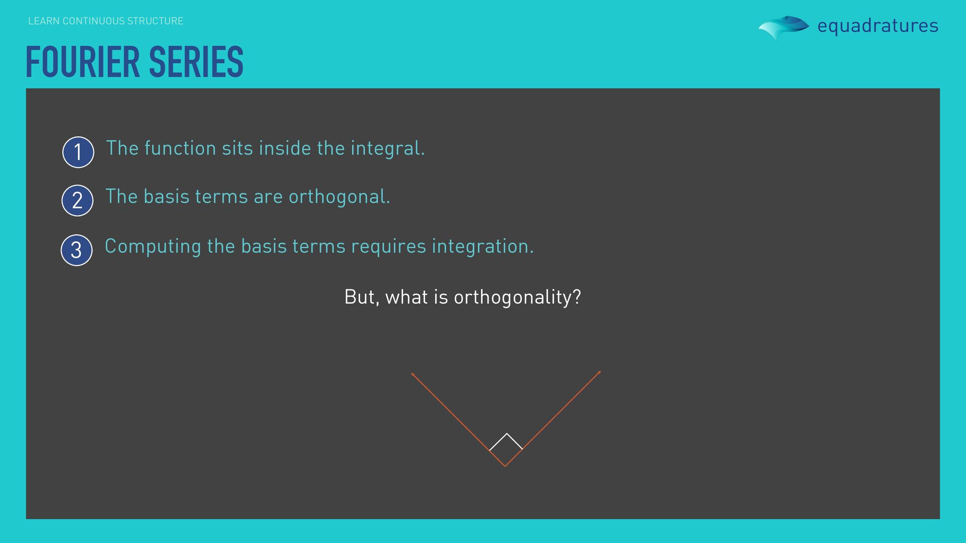
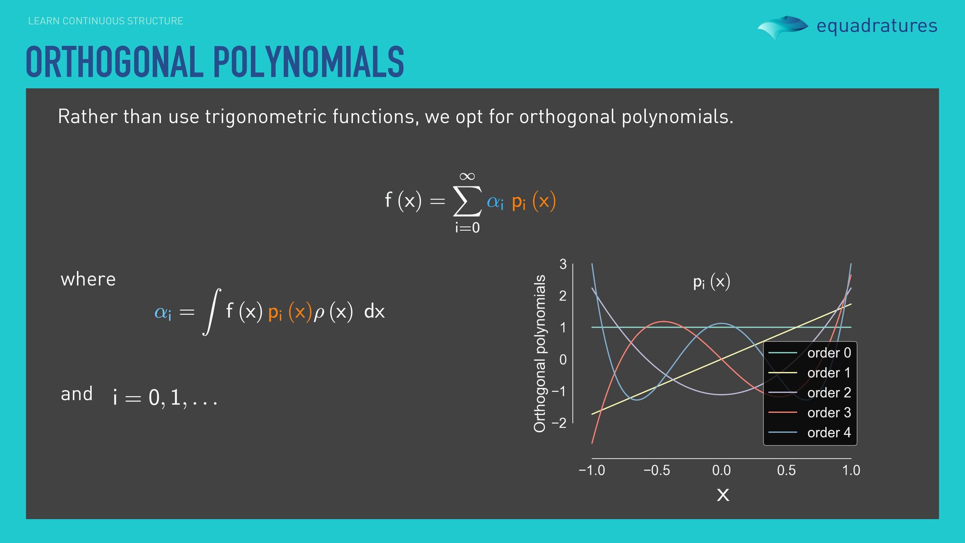
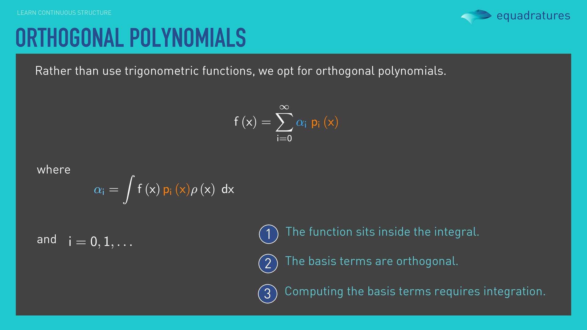
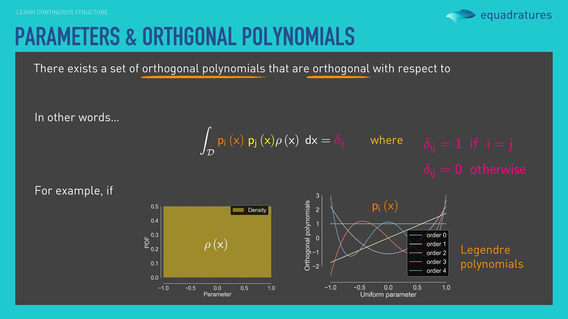
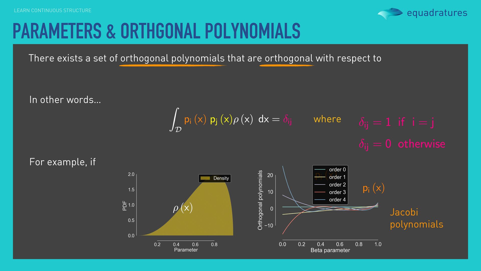
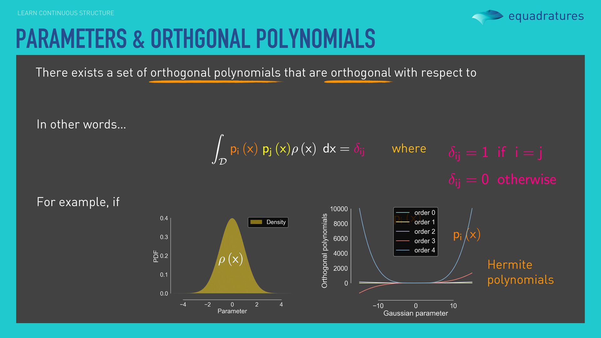
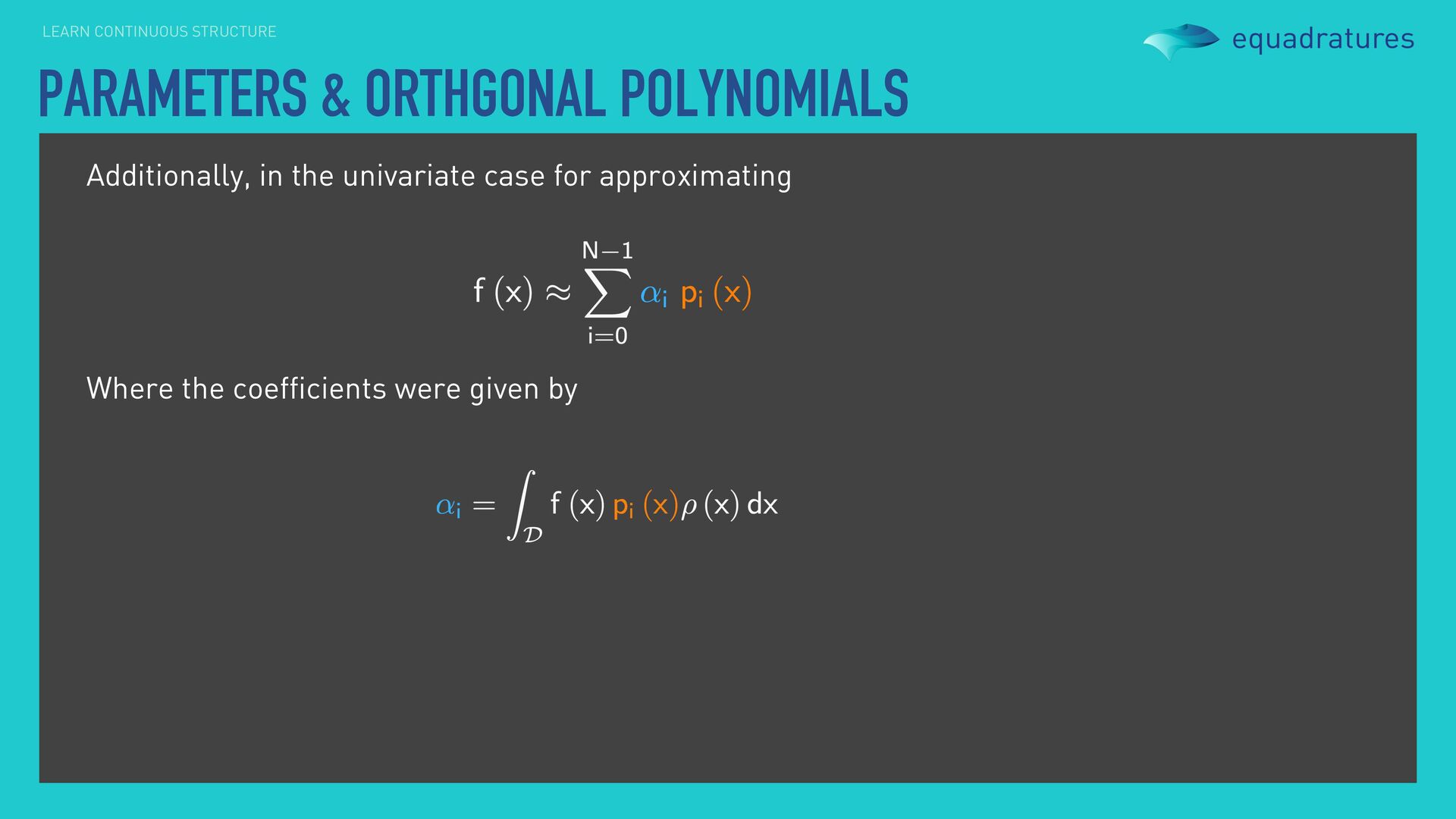
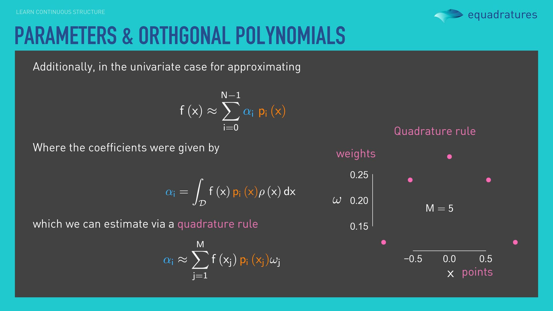
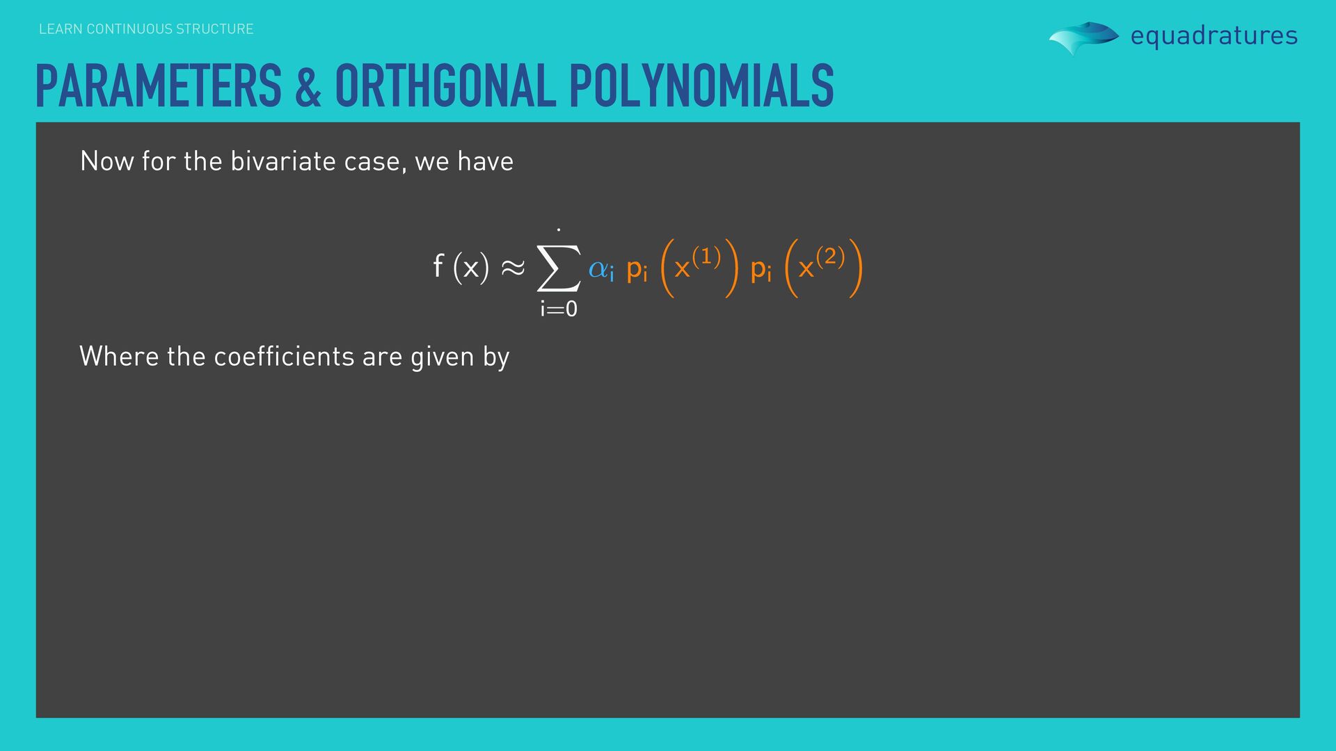
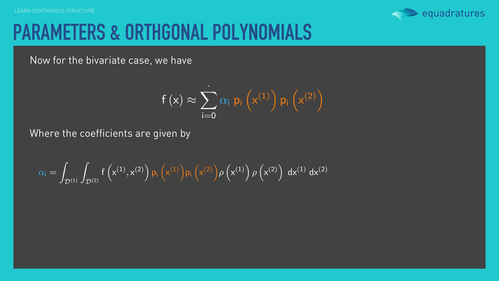
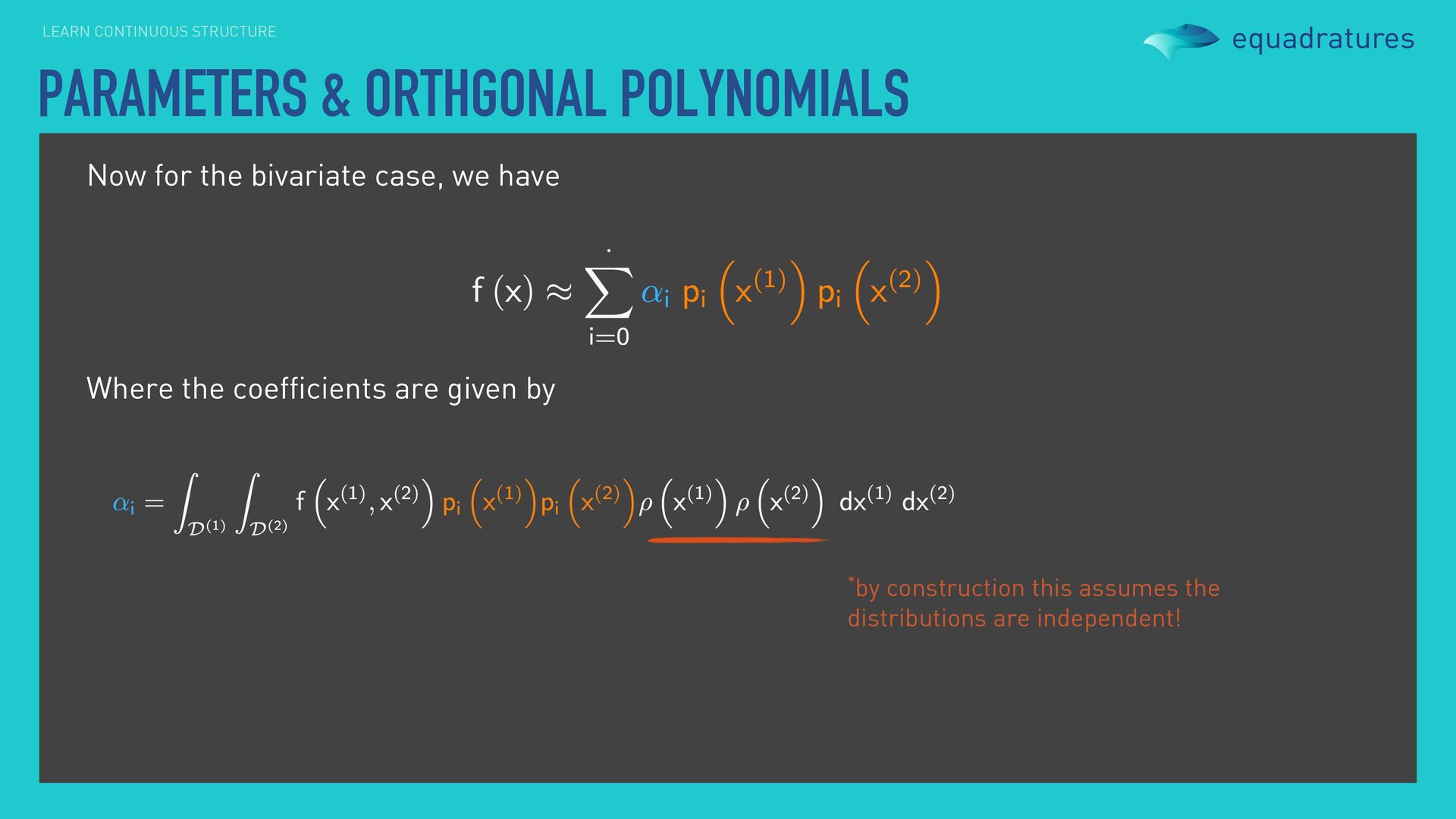
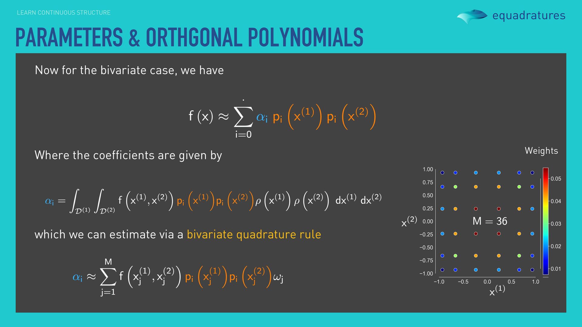
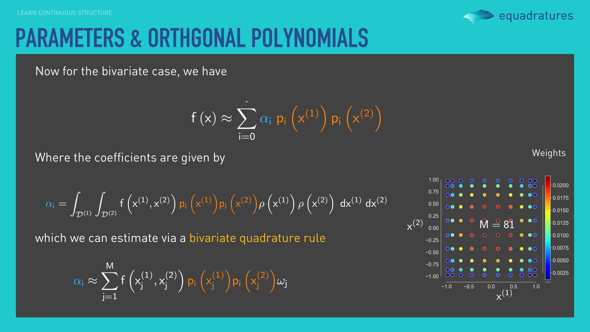
we opt for orthogonal polynomials. where and The function sits inside the integral. 1 The basis terms are orthogonal. 2 Computing the basis terms requires integration. 3
of orthogonal polynomials, we need to integrate to estimate its coefficients. Moreover, we need to ascertain the level of truncation required. ORTHOGONAL POLYNOMIALS
of orthogonal polynomials, we need to integrate to estimate its coefficients. Moreover, we need to ascertain the level of truncation required. But, before we move forward, we need to understand these polynomials more intimately. ORTHOGONAL POLYNOMIALS
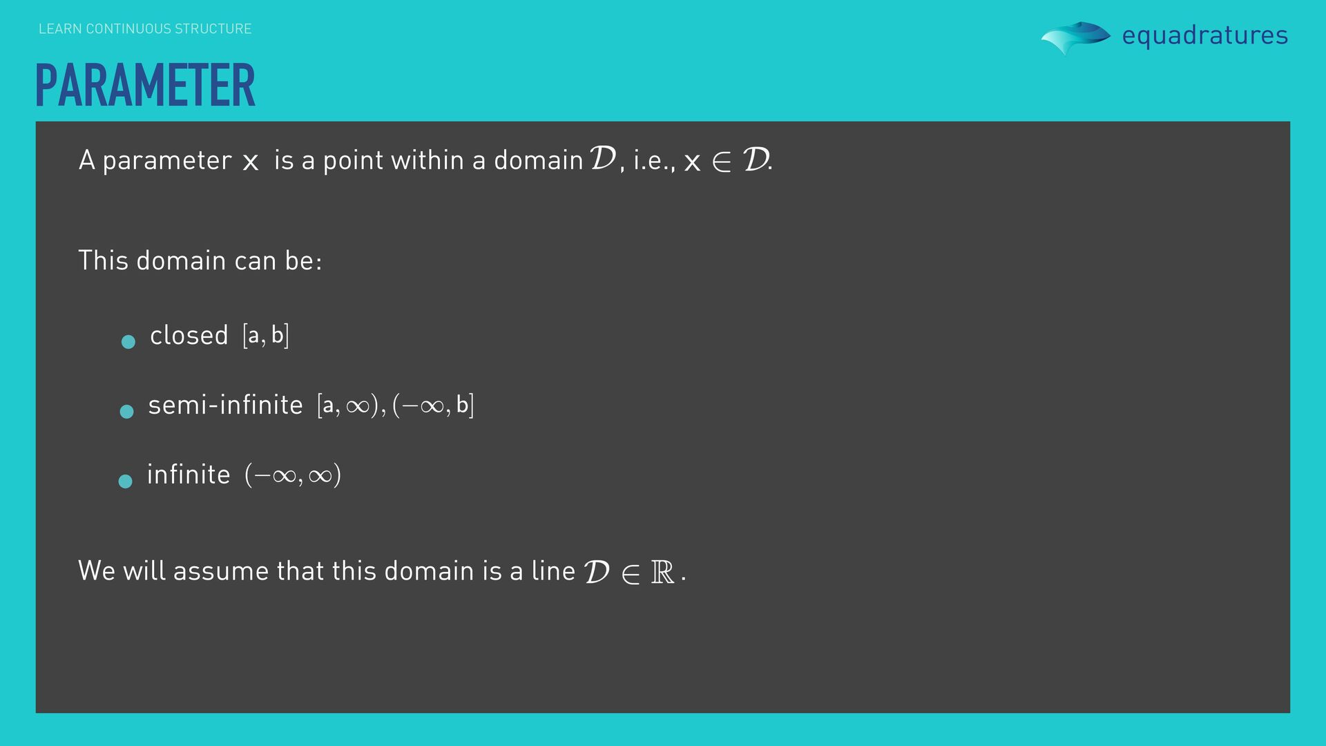
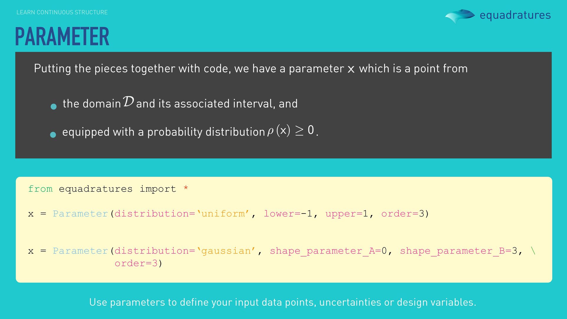
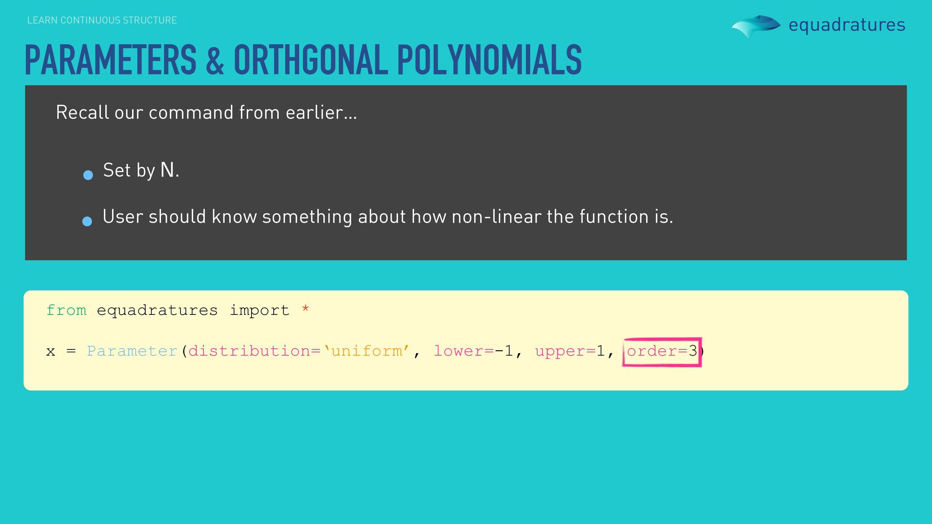
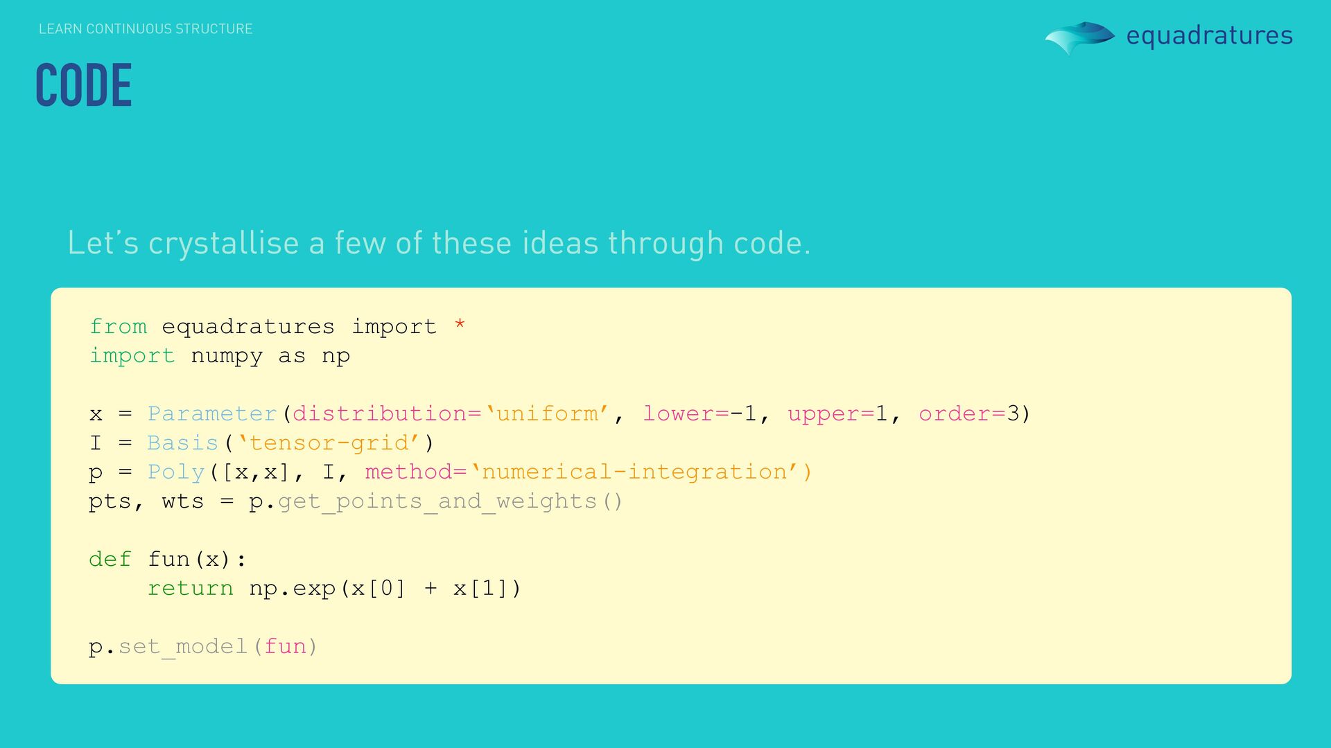
we have a parameter which is a point from the domain and its associated interval, and equipped with a probability distribution . from equadratures import * x = Parameter(distribution=‘uniform’, lower=-1, upper=1, order=3) x = Parameter(distribution=‘gaussian’, shape_parameter_A=0, shape_parameter_B=3, \ order=3) Use parameters to define your input data points, uncertainties or design variables.
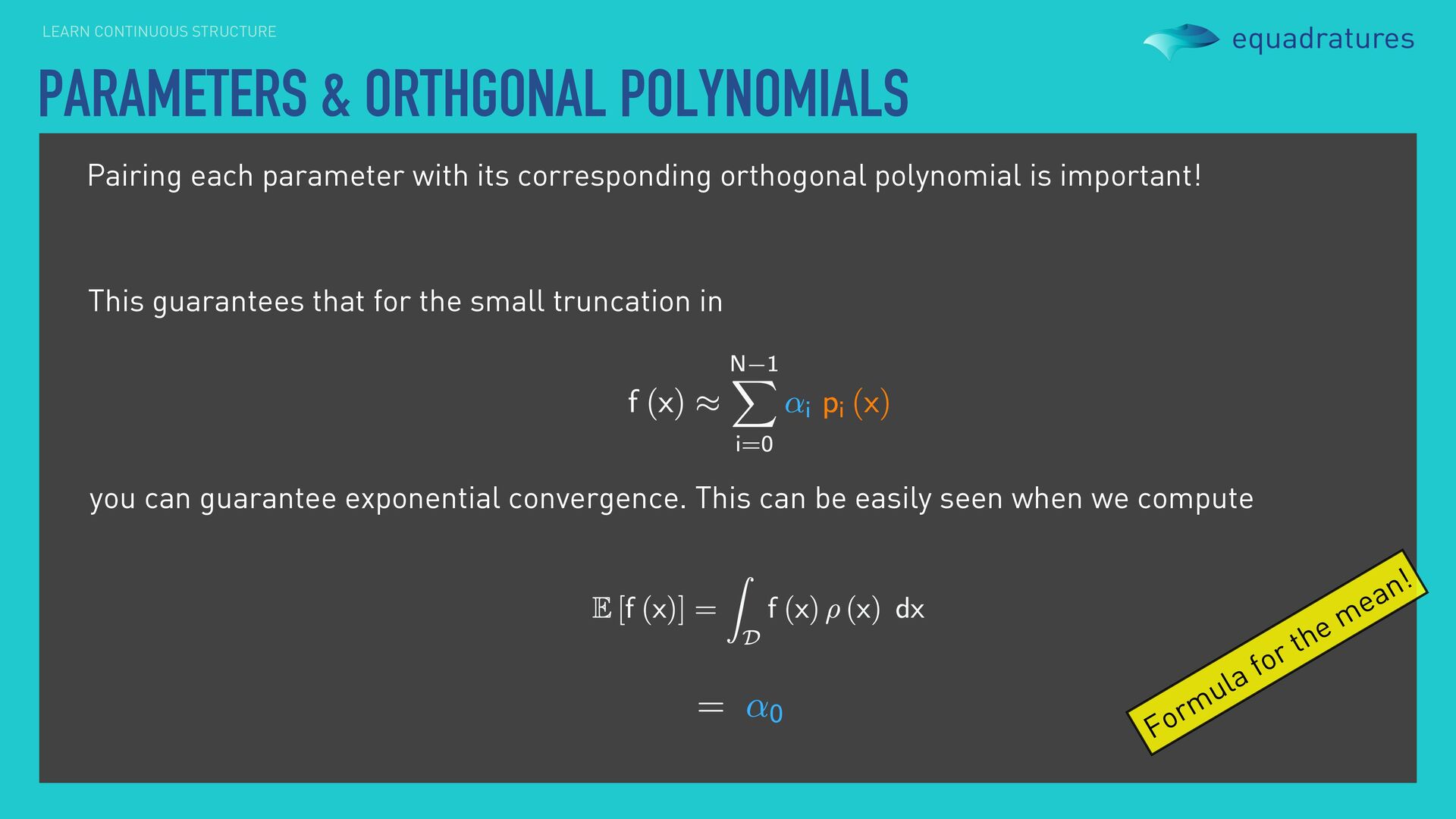
with its corresponding orthogonal polynomial is important! This guarantees that for the small truncation in you can guarantee exponential convergence. This can be easily seen when we compute Formula for the mean!
with its corresponding orthogonal polynomial is important! This guarantees that for the small truncation in you can guarantee exponential convergence. This can be easily seen when we compute Formula for the variance!
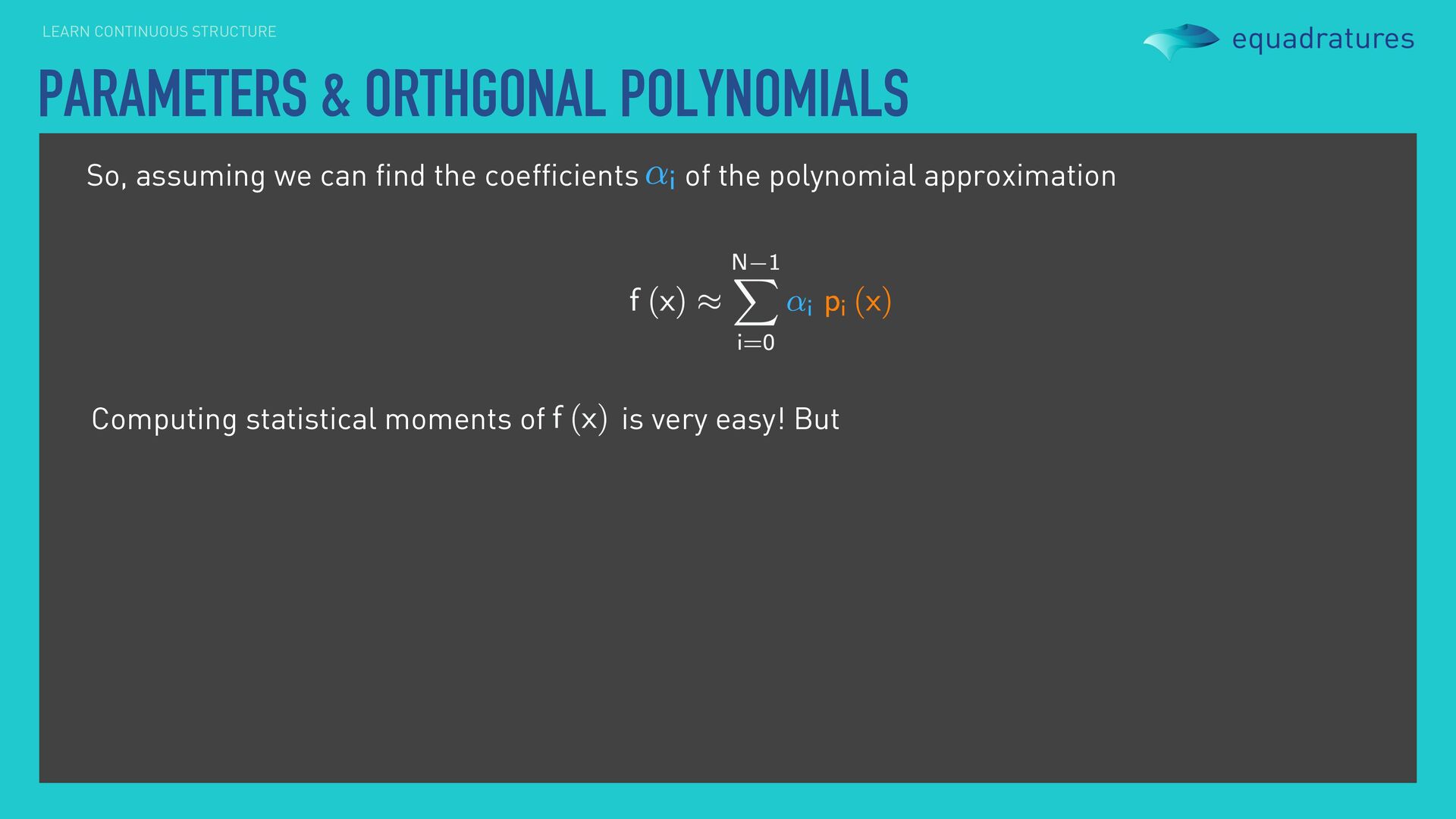
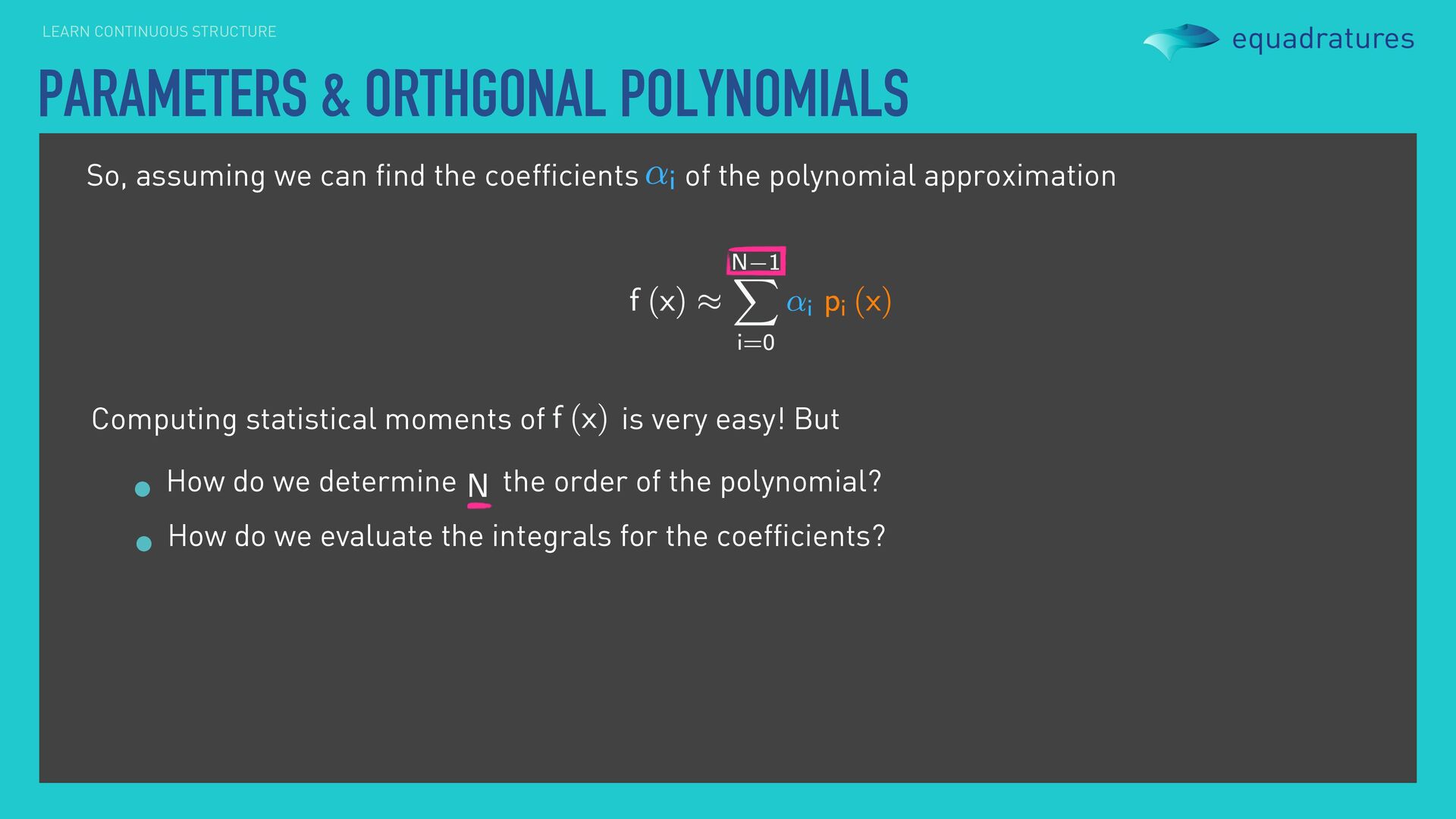
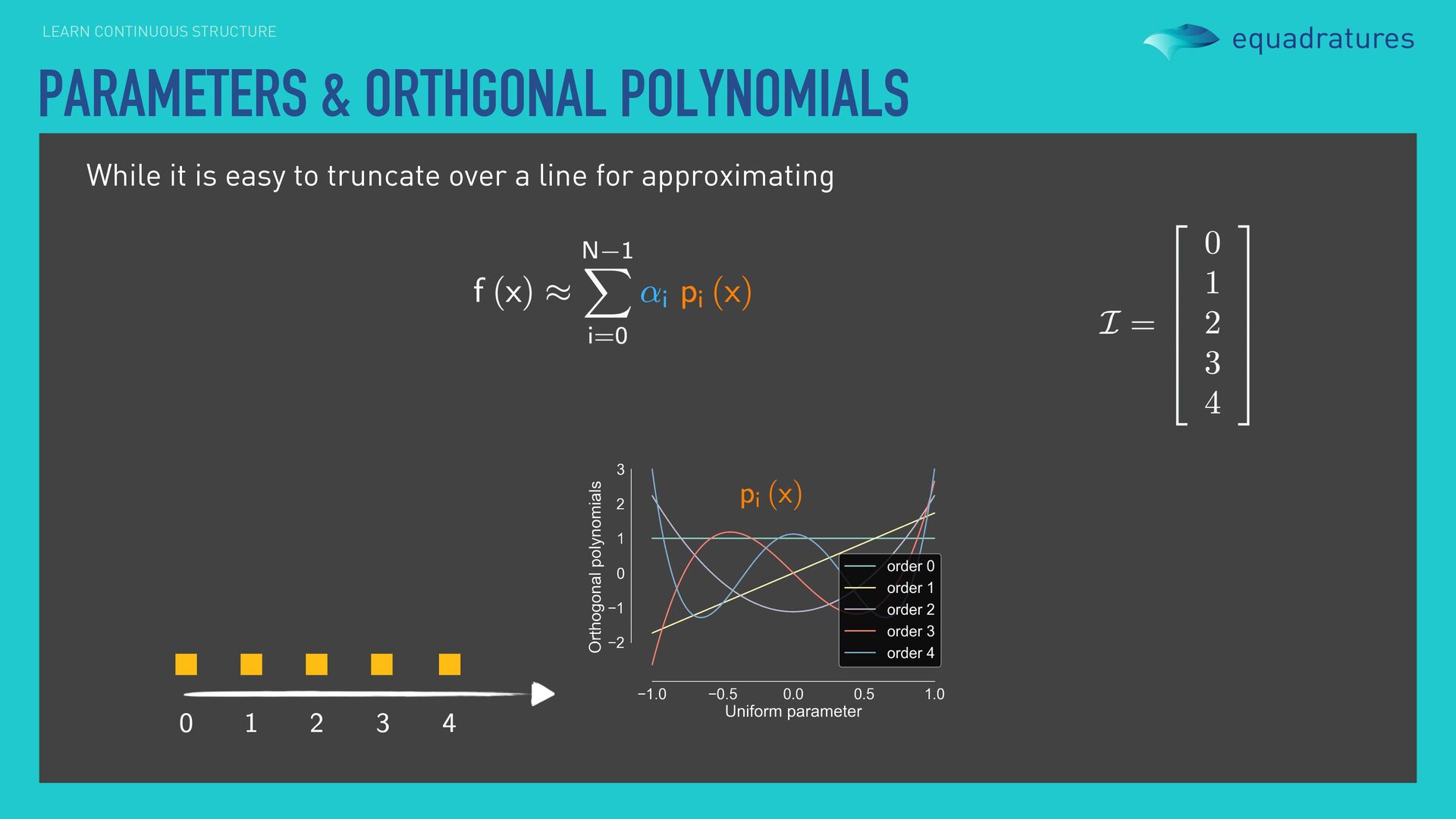
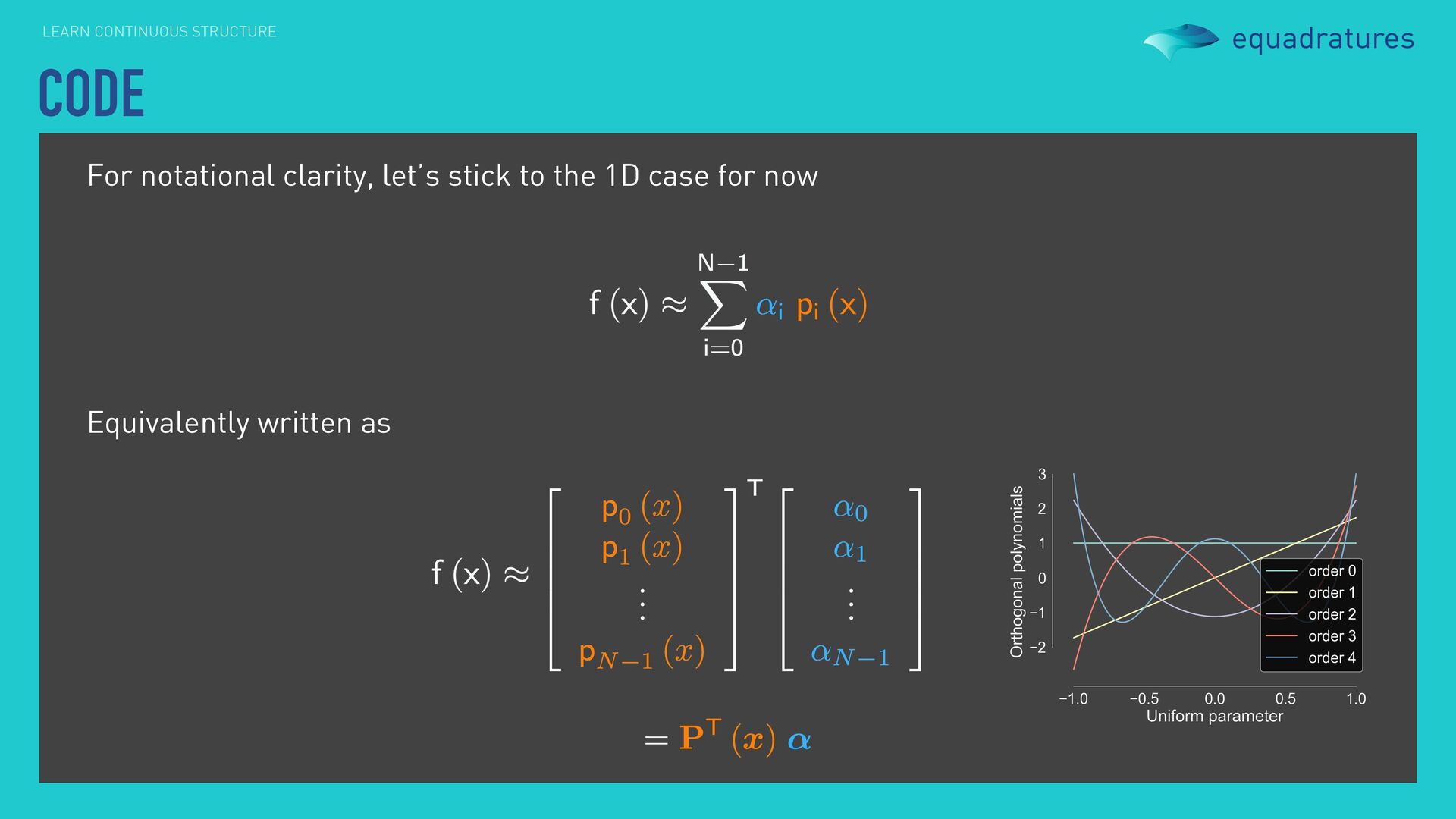
can find the coefficients of the polynomial approximation Computing statistical moments of is very easy! But How do we determine the order of the polynomial? How do we evaluate the integrals for the coefficients?
from earlier… Set by . User should know something about how non-linear the function is. from equadratures import * x = Parameter(distribution=‘uniform’, lower=-1, upper=1, order=3)
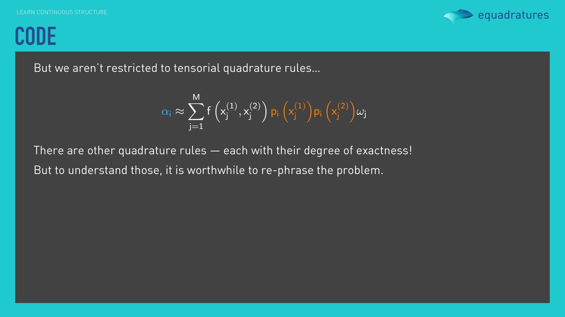
quadrature rules… There are other quadrature rules — each with their degree of exactness! But to understand those, it is worthwhile to re-phrase the problem.
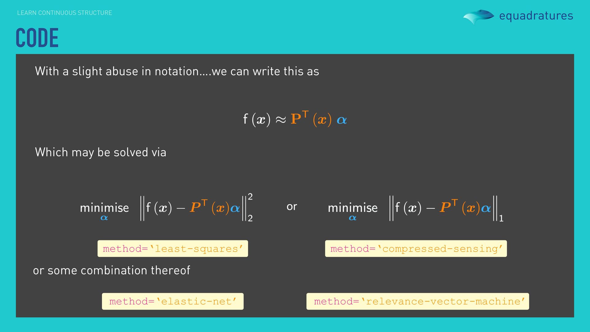
can write this as Which may be solved via or or some combination thereof method=‘least-squares’ method=‘compressed-sensing’ method=‘elastic-net’ method=‘relevance-vector-machine’
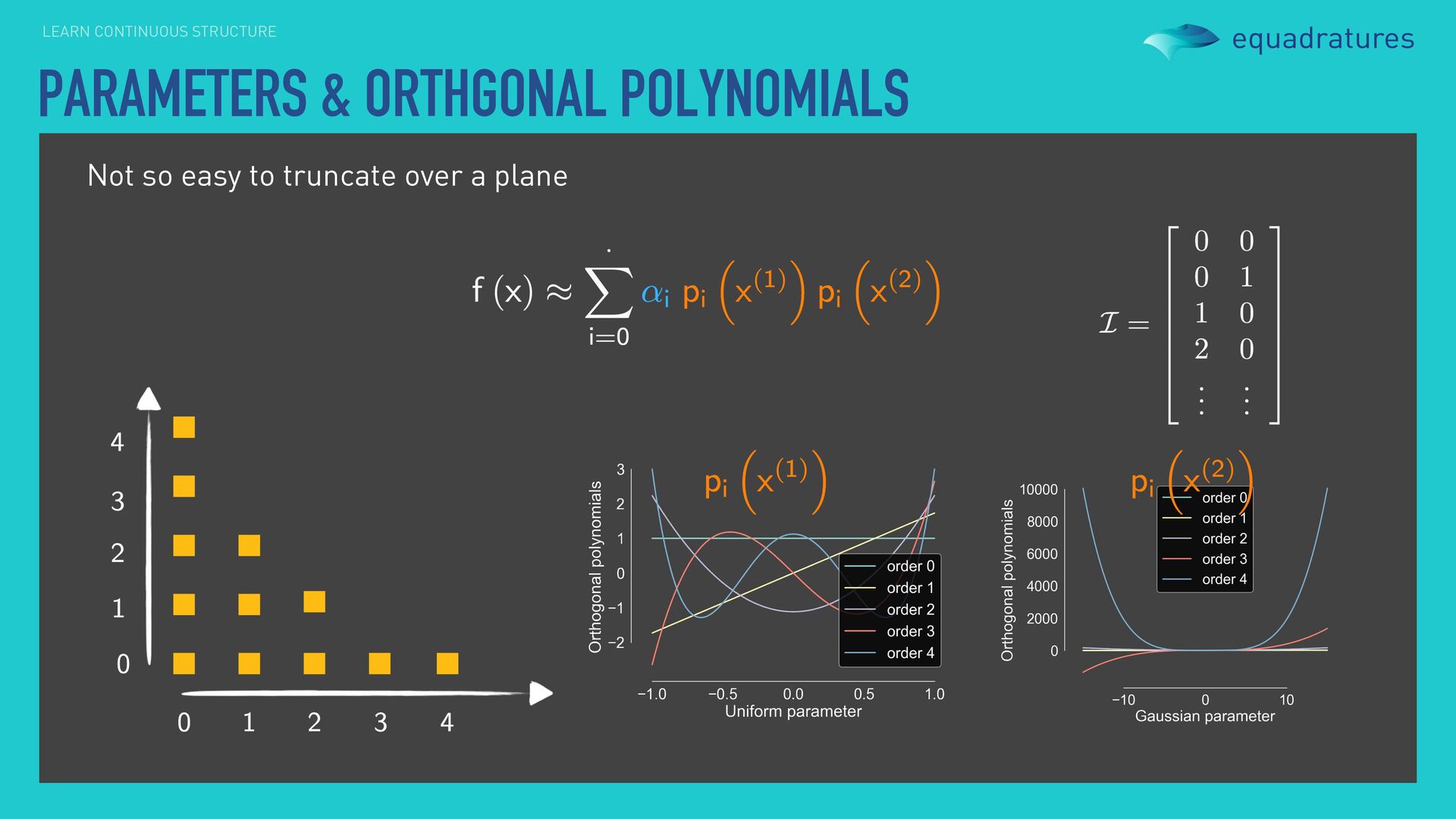
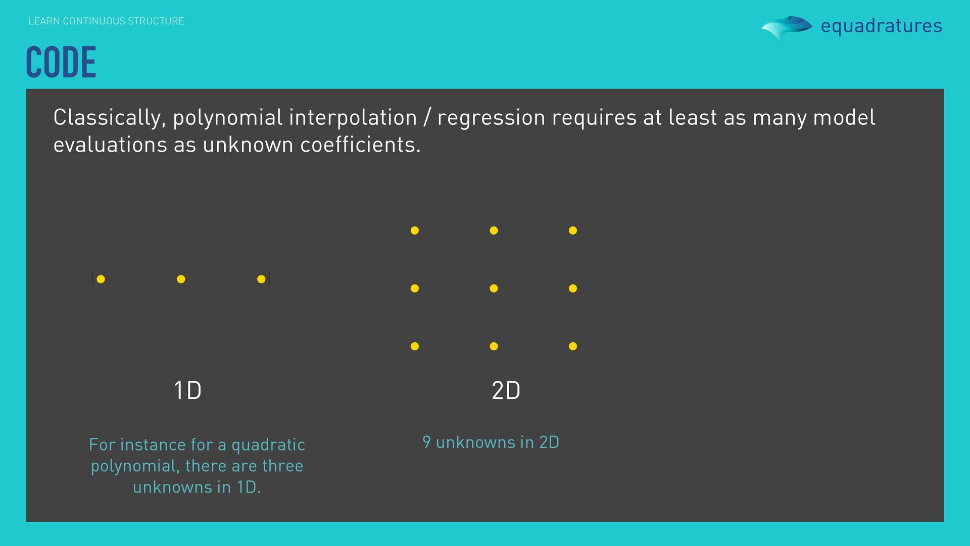
at least as many model evaluations as unknown coefficients. 1D 2D For instance for a quadratic polynomial, there are three unknowns in 1D. 9 unknowns in 2D
at least as many model evaluations as unknown coefficients. 1D 2D For instance for a quadratic polynomial, there are three unknowns in 1D. 9 unknowns in 2D 3D 27 unknowns in 3D
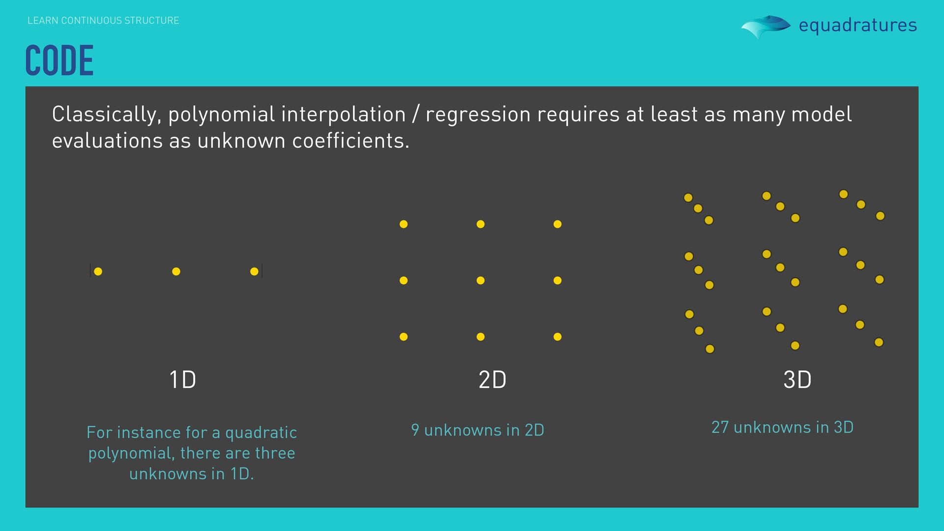
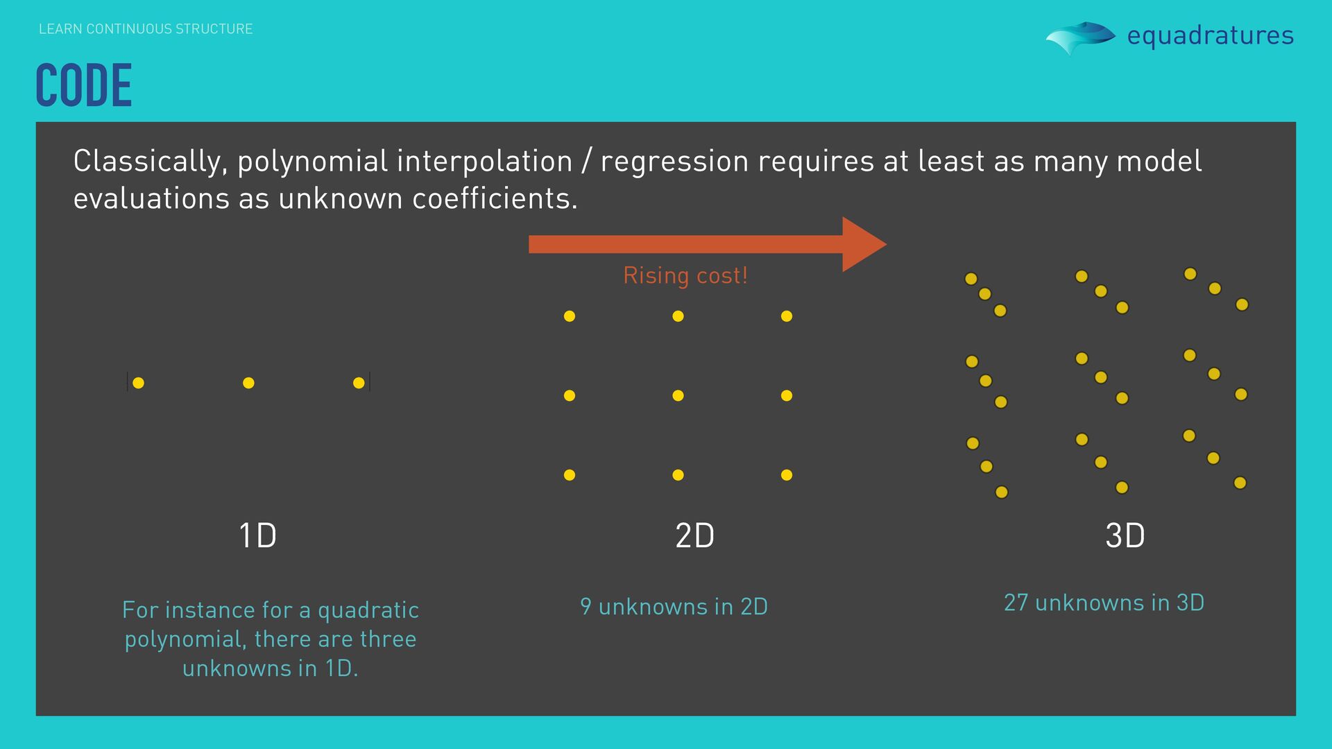
at least as many model evaluations as unknown coefficients. 1D 2D For instance for a quadratic polynomial, there are three unknowns in 1D. 9 unknowns in 2D 3D 27 unknowns in 3D Rising cost!