Data-Driven Dimension Reduction

An introduction to PCA, active subspaces, and ridge approximations

Transcript

1. DATA-DRIVEN DIMENSION REDUCTION Pranay Seshadri Associate Professor in Aerospace Engineering Georgia Institute of Technology
2. DATA-DRIVEN DIMENSION REDUCTION ACKNOWLEDGEMENTS Much of the code was written by Henry Yuchi, Chun Yui Wong, with further edits made by Ashley Scillitoe. We are grateful to Paul Constantine — for without him, this deck wouldn’t exist. FOLKS WHO HAVE CONTRIBUTED
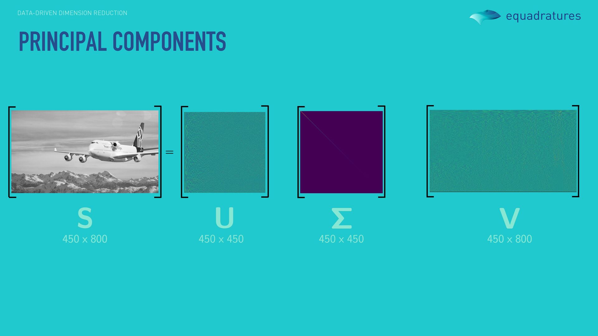
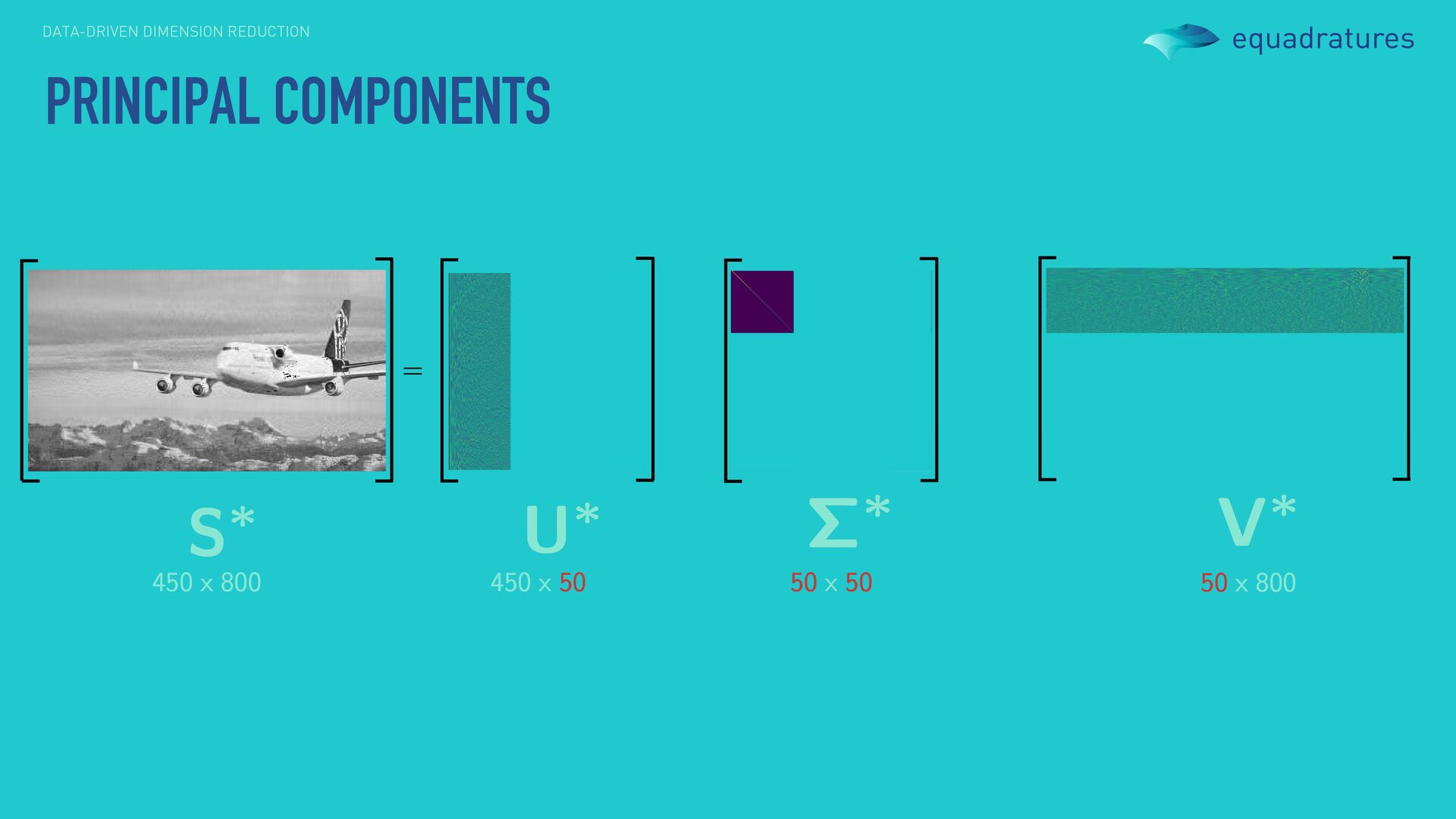
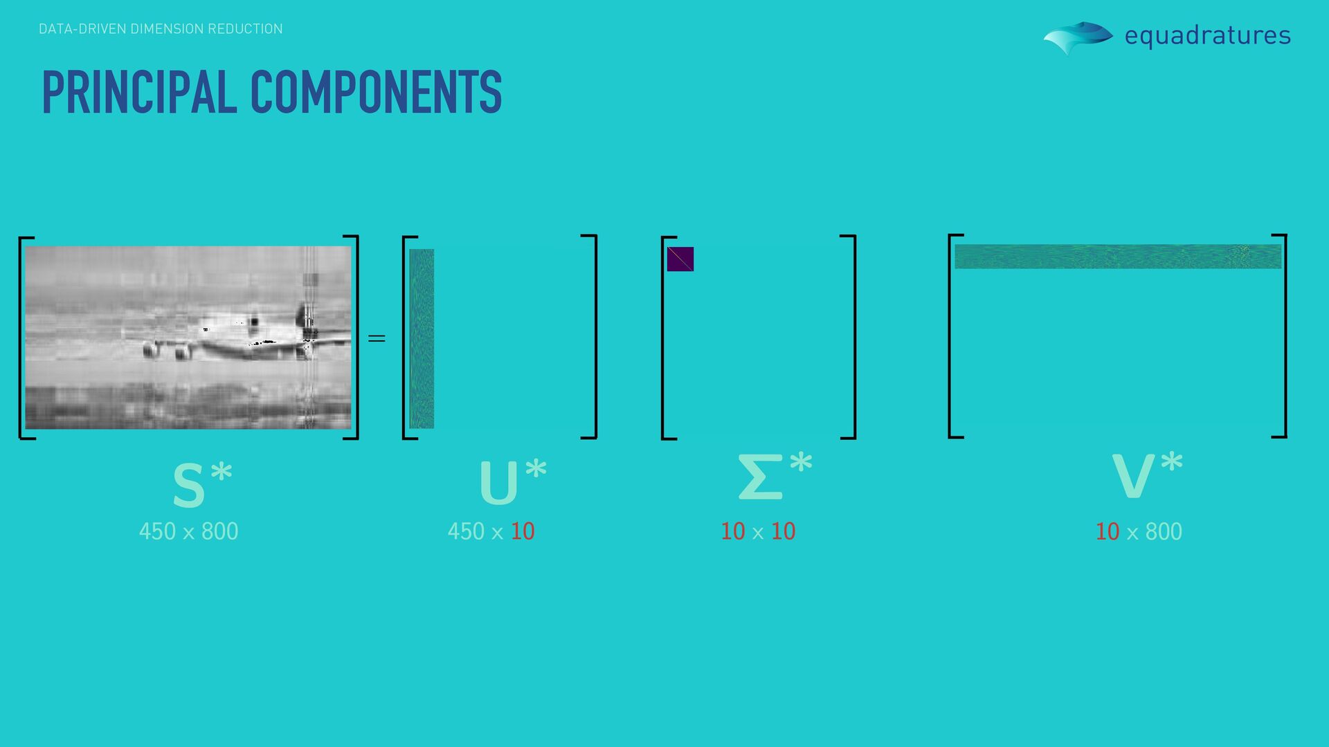
3. DATA-DRIVEN DIMENSION REDUCTION INTRODUCTION The trouble is that high-dimensional problems are inevitable and unavoidable. Thankfully, equadratures has a few utilities that may be useful. But before delving into them, it will be useful to talk about ideas like principal components analysis (PCA) and more generally the singular value decomposition. A FEW WORDS
4. DATA-DRIVEN DIMENSION REDUCTION OVERVIEW 1. PRINCIPAL COMPONENTS 2. A SIMPLE EXPERIMENT 3. PROJECTIONS & ZONOTOPES 4. ACTIVE SUBSPACES 5. RIDGE APPROXIMATIONS
5. DATA-DRIVEN DIMENSION REDUCTION Image source: Rolls-Royce Flickr
6. DATA-DRIVEN DIMENSION REDUCTION PRINCIPAL COMPONENTS
7. DATA-DRIVEN DIMENSION REDUCTION diagonal matrix of singular values Number of rows Singular values PRINCIPAL COMPONENTS
8. DATA-DRIVEN DIMENSION REDUCTION PRINCIPAL COMPONENTS
9. DATA-DRIVEN DIMENSION REDUCTION PRINCIPAL COMPONENTS
10. DATA-DRIVEN DIMENSION REDUCTION PRINCIPAL COMPONENTS
11. DATA-DRIVEN DIMENSION REDUCTION PRINCIPAL COMPONENTS
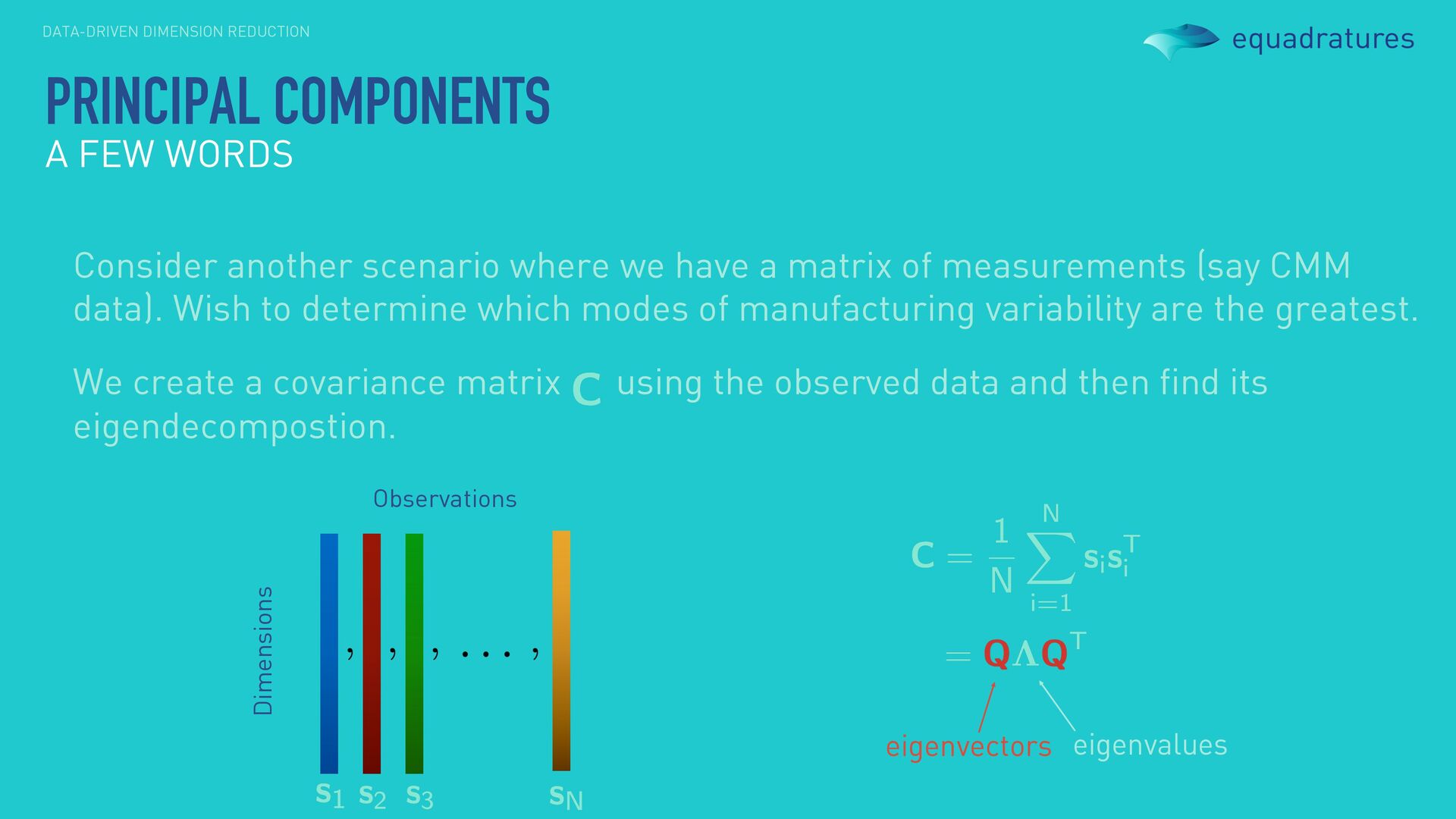
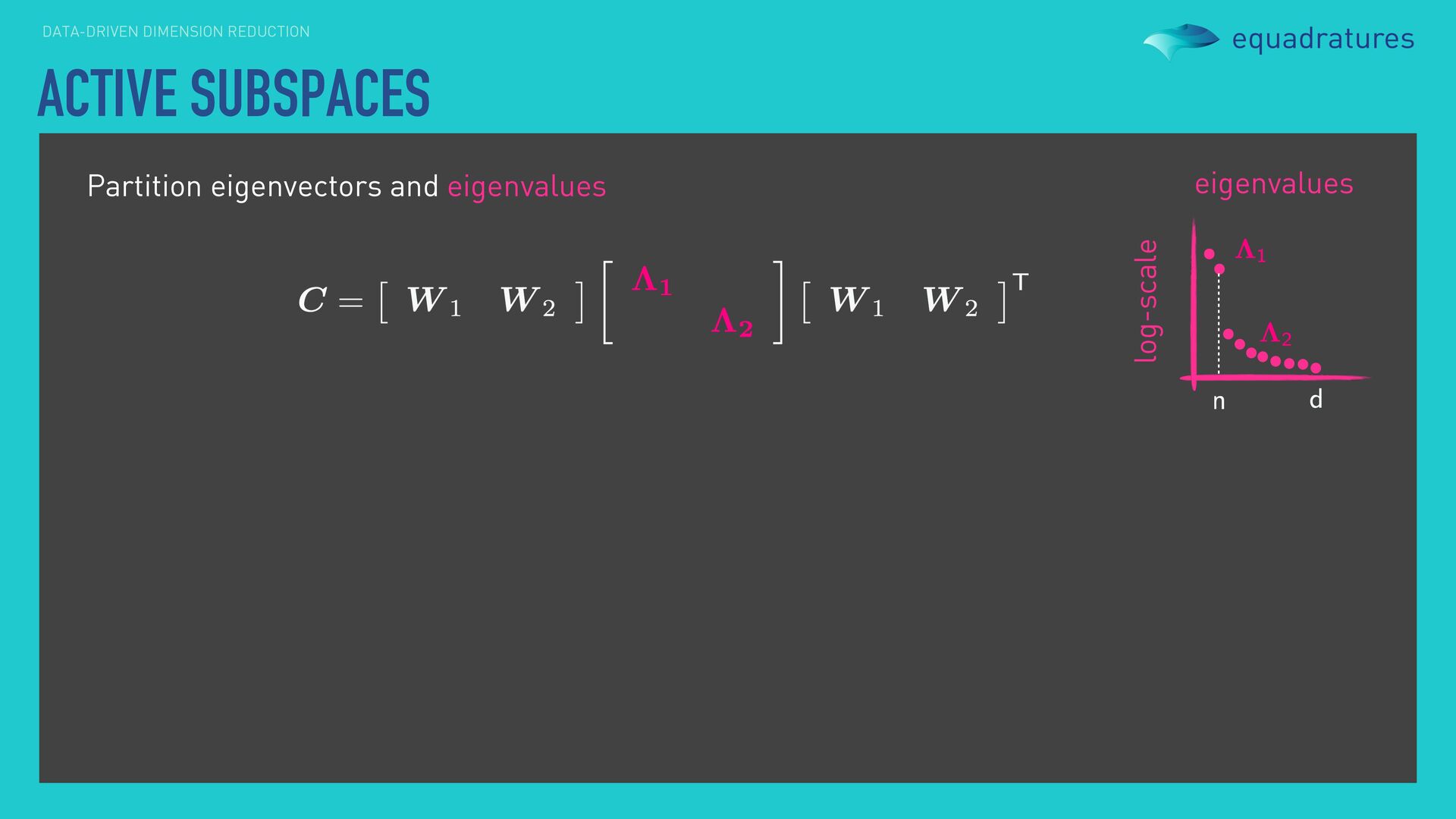
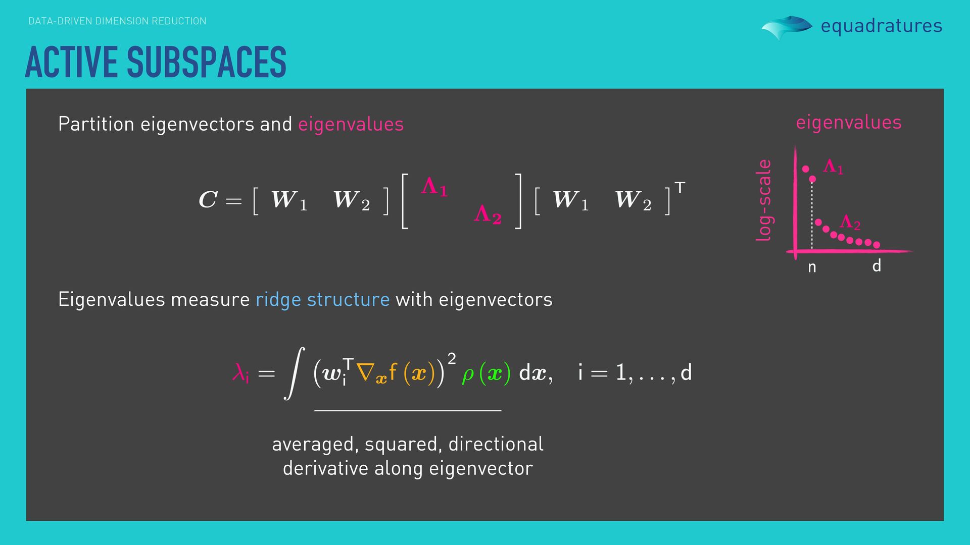
12. DATA-DRIVEN DIMENSION REDUCTION PRINCIPAL COMPONENTS Consider another scenario where we have a matrix of measurements (say CMM data). Wish to determine which modes of manufacturing variability are the greatest. We create a covariance matrix using the observed data and then find its eigendecompostion. A FEW WORDS eigenvectors eigenvalues Observations Dimensions
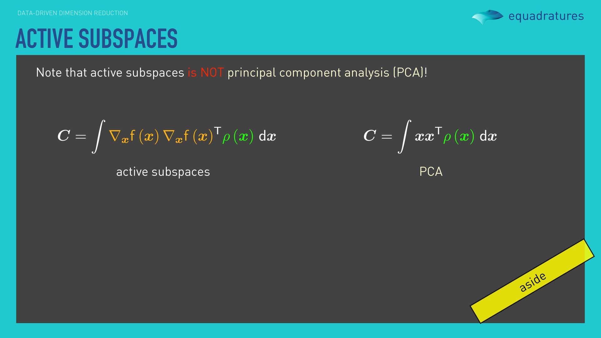
13. DATA-DRIVEN DIMENSION REDUCTION PRINCIPAL COMPONENTS SUMMARISING THOUGHTS *Candés, Li, Ma, Wright (2011) Robust principal component analysis? J. ACM. *Schölkopf, Smola, Müller (1997) Kernel principal component analysis. Springer. Rather than apply principal components to a single image, we can apply it to numerous images to find dominant linear directions across all the images. Utility is not restricted to images and videos, but to any matrix / vector database. More robust and nonlinear variants also exist. However, we can’t really use this if we are interested in input-output pairs. For instance, computer experiments are usually carried out via a uniform design of experiment. Naïvely applying PCA to the inputs does not facilitate output-driven dimension reduction.
14. DATA-DRIVEN DIMENSION REDUCTION OVERVIEW 1. PRINCIPAL COMPONENTS 2. A SIMPLE EXPERIMENT 3. PROJECTIONS & ZONOTOPES 4. ACTIVE SUBSPACES 5. RIDGE APPROXIMATIONS
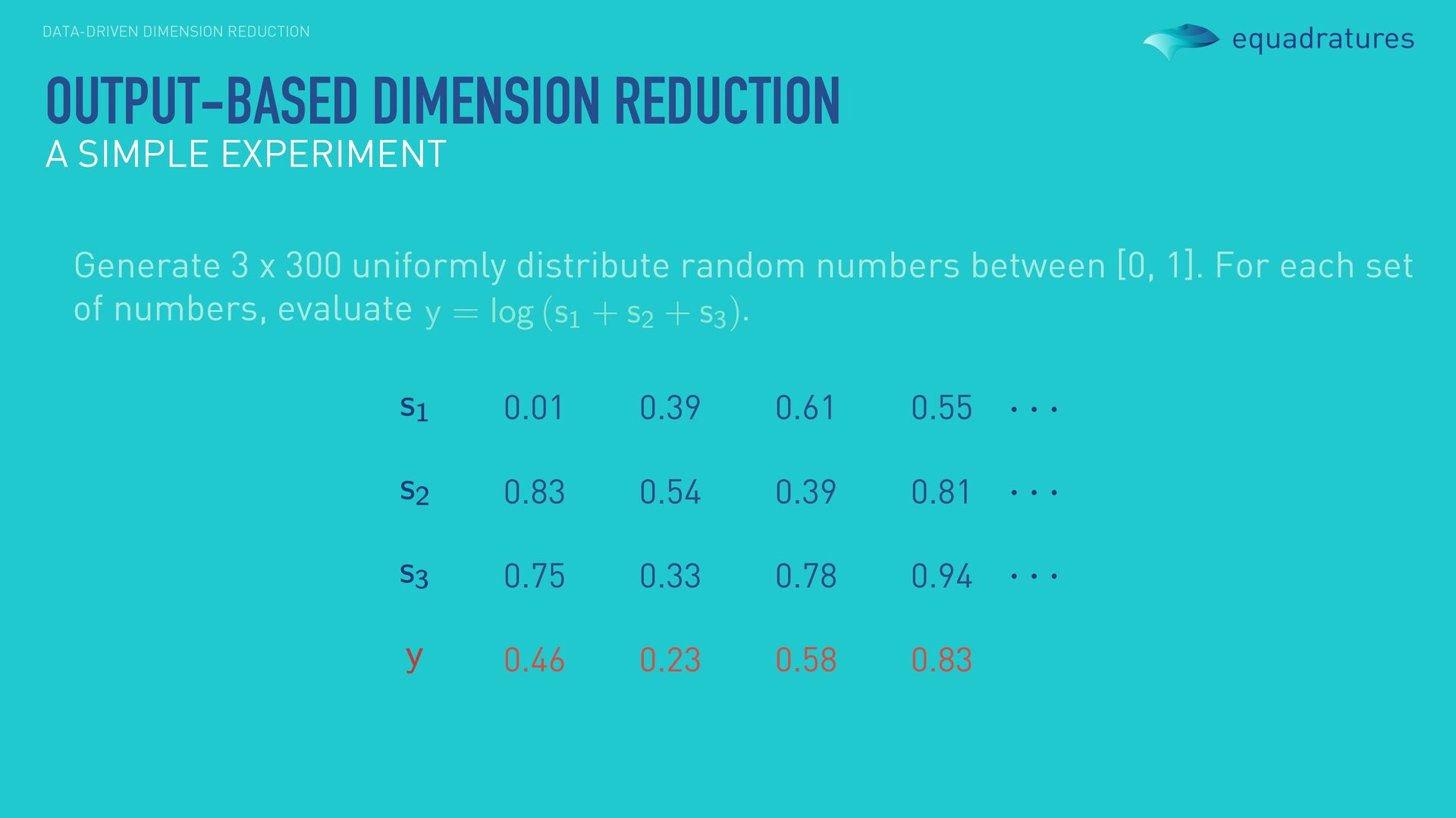
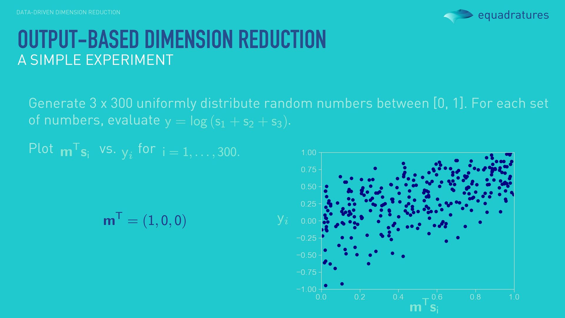
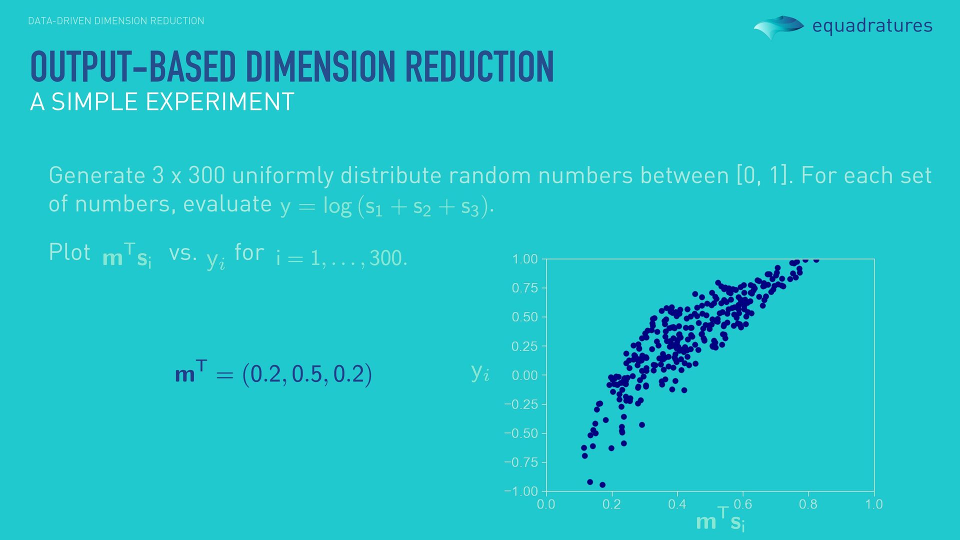
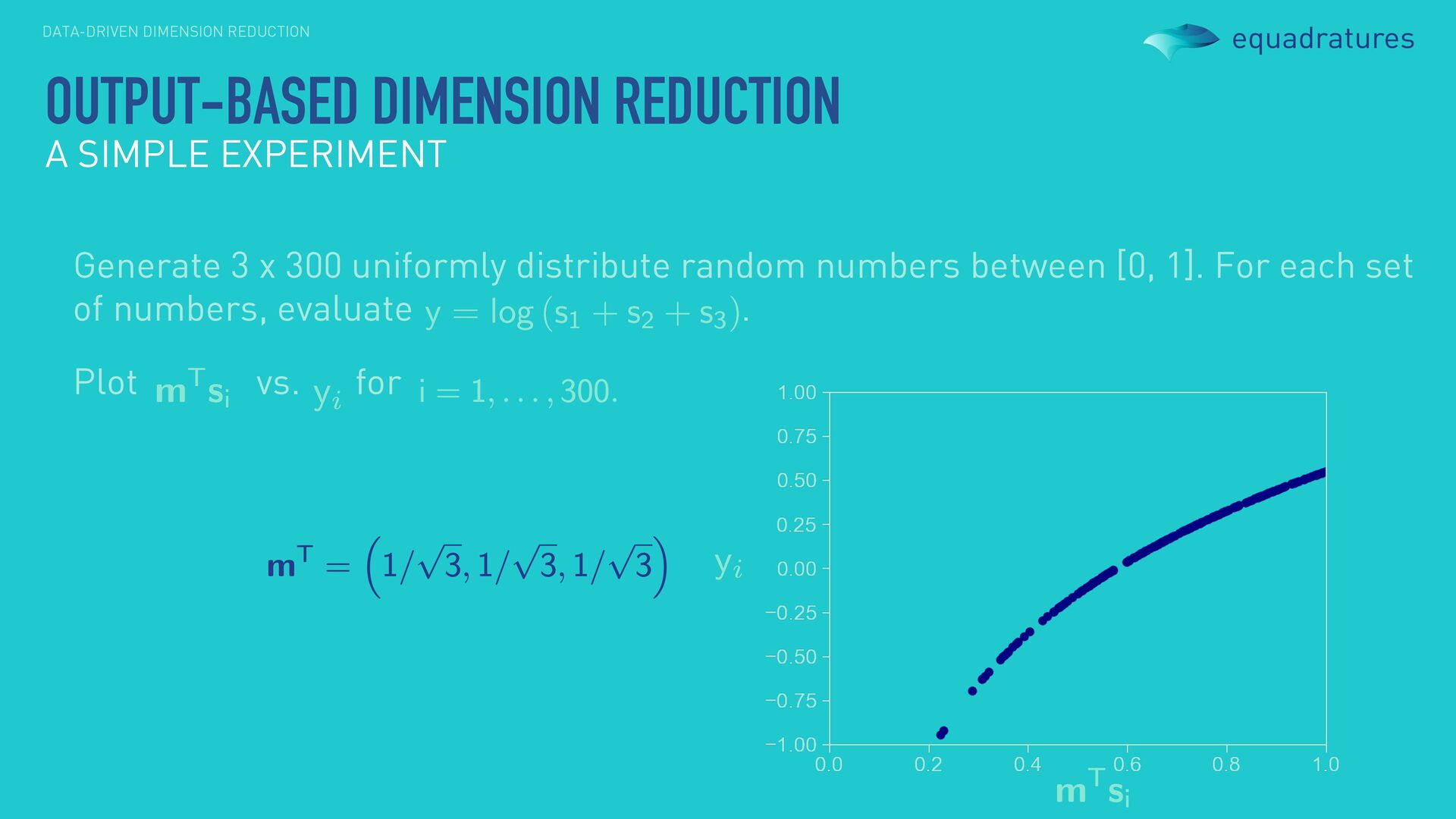
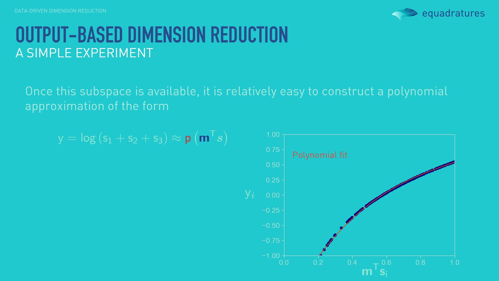
15. DATA-DRIVEN DIMENSION REDUCTION 0.01 0.39 0.61 0.55 0.83 0.54 0.39 0.81 0.75 0.33 0.78 0.94 0.46 0.23 0.58 0.83 Generate 3 x 300 uniformly distribute random numbers between [0, 1]. For each set of numbers, evaluate . OUTPUT-BASED DIMENSION REDUCTION A SIMPLE EXPERIMENT
16. DATA-DRIVEN DIMENSION REDUCTION Generate 3 x 300 uniformly distribute random numbers between [0, 1]. For each set of numbers, evaluate . Plot vs. for OUTPUT-BASED DIMENSION REDUCTION A SIMPLE EXPERIMENT
17. DATA-DRIVEN DIMENSION REDUCTION Generate 3 x 300 uniformly distribute random numbers between [0, 1]. For each set of numbers, evaluate . Plot vs. for OUTPUT-BASED DIMENSION REDUCTION A SIMPLE EXPERIMENT
18. DATA-DRIVEN DIMENSION REDUCTION Generate 3 x 300 uniformly distribute random numbers between [0, 1]. For each set of numbers, evaluate . Plot vs. for OUTPUT-BASED DIMENSION REDUCTION A SIMPLE EXPERIMENT
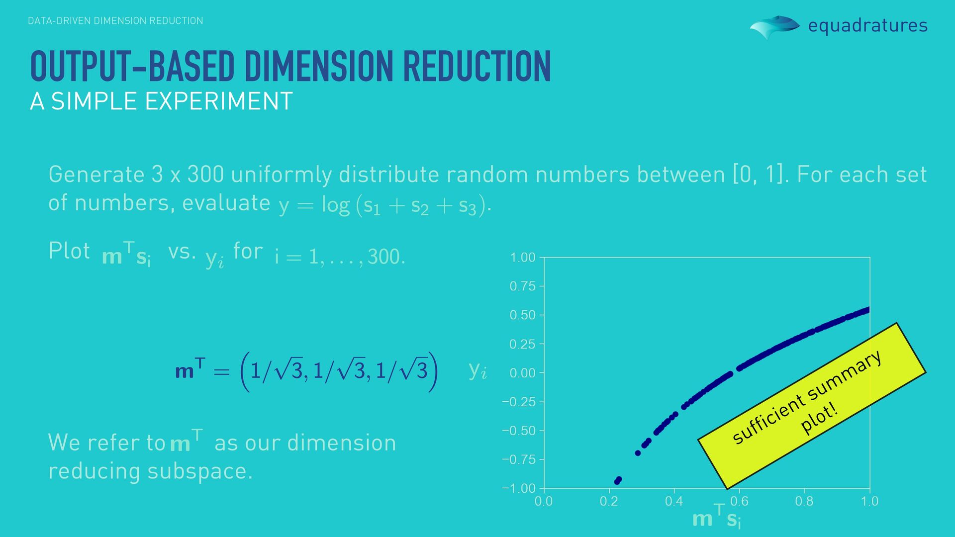
19. DATA-DRIVEN DIMENSION REDUCTION Generate 3 x 300 uniformly distribute random numbers between [0, 1]. For each set of numbers, evaluate . Plot vs. for OUTPUT-BASED DIMENSION REDUCTION A SIMPLE EXPERIMENT We refer to as our dimension reducing subspace. sufficient summary plot!
20. DATA-DRIVEN DIMENSION REDUCTION Once this subspace is available, it is relatively easy to construct a polynomial approximation of the form OUTPUT-BASED DIMENSION REDUCTION A SIMPLE EXPERIMENT Polynomial fit
21. DATA-DRIVEN DIMENSION REDUCTION OUTPUT-BASED DIMENSION REDUCTION ANALOGOUS TO A SINGLE LAYER NEURAL NETWORK Hidden layer Inputs Output
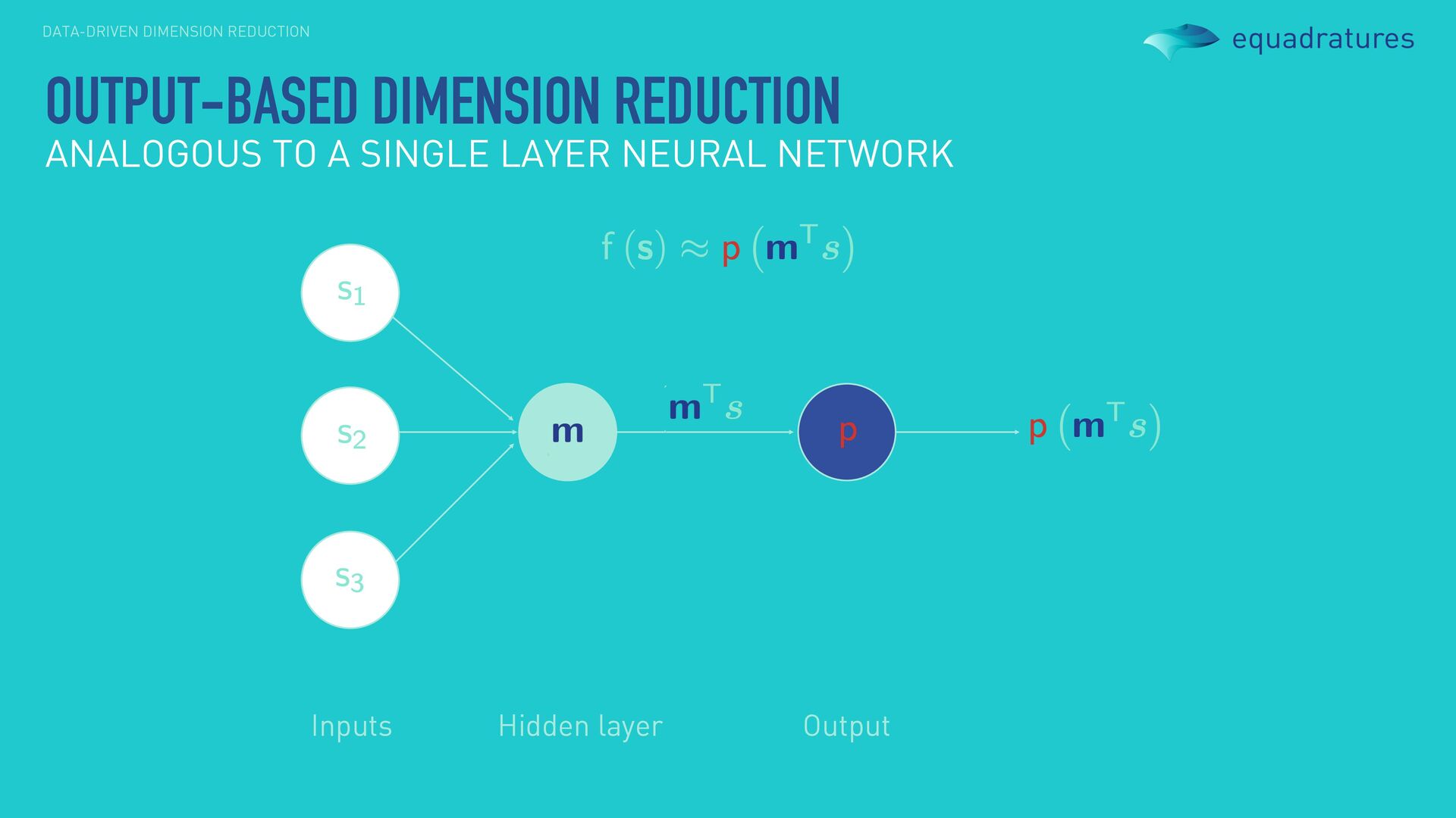
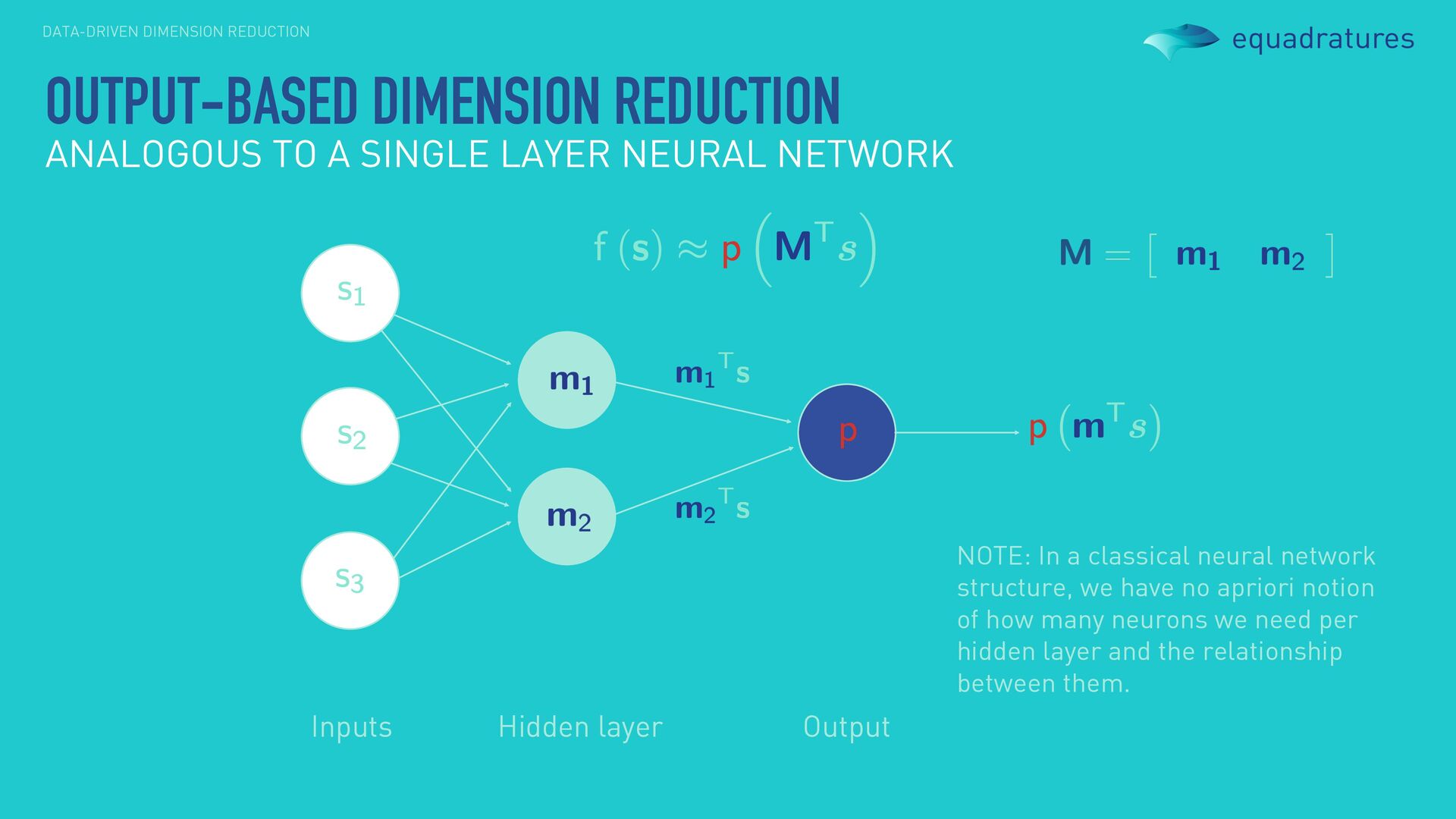
22. DATA-DRIVEN DIMENSION REDUCTION OUTPUT-BASED DIMENSION REDUCTION ANALOGOUS TO A SINGLE LAYER NEURAL NETWORK Hidden layer Inputs Output NOTE: In a classical neural network structure, we have no apriori notion of how many neurons we need per hidden layer and the relationship between them.
23. DATA-DRIVEN DIMENSION REDUCTION OVERVIEW 1. PRINCIPAL COMPONENTS 2. A SIMPLE EXPERIMENT 3. PROJECTIONS & ZONOTOPES 4. ACTIVE SUBSPACES 5. RIDGE APPROXIMATIONS
24. DATA-DRIVEN DIMENSION REDUCTION PROJECTIONS & ZONOTOPES SUBSPACE-BASED [LINEAR] PROJECTIONS Consider the d-dimensional input observations to some computational model, i.e., .
25. DATA-DRIVEN DIMENSION REDUCTION PROJECTIONS & ZONOTOPES SUBSPACE-BASED [LINEAR] PROJECTIONS Human A 3D object. Shadow A 2D projection of a 3D object. Be aware: understanding high- dimensional spaces is very important!
26. DATA-DRIVEN DIMENSION REDUCTION PROJECTIONS & ZONOTOPES SUBSPACE-BASED [LINEAR] PROJECTIONS Human A 3D object. Shadow A 2D projection of a 3D object. Consider the projection of a cube on a plane, it can either be a square or hexagon. Be aware: understanding high- dimensional spaces is very important!
27. DATA-DRIVEN DIMENSION REDUCTION PROJECTIONS & ZONOTOPES SUBSPACE-BASED [LINEAR] PROJECTIONS Generate random samples within a 𝖽 = 𝟥 dimensional cube and project using a random orthogonal projection. “Zonotope” Projection of hypercube on a plane
28. DATA-DRIVEN DIMENSION REDUCTION PROJECTIONS & ZONOTOPES SUBSPACE-BASED [LINEAR] PROJECTIONS Generate random samples within a 𝖽 = 𝟣𝟢 dimensional cube and project using a random orthogonal projection. “Zonotope” Projection of hypercube on a plane
29. DATA-DRIVEN DIMENSION REDUCTION PROJECTIONS & ZONOTOPES SUBSPACE-BASED [LINEAR] PROJECTIONS Generate random samples within a 𝖽 = 𝟧𝟢 dimensional cube and project using a random orthogonal projection. “Zonotope” Projection of hypercube on a plane
30. DATA-DRIVEN DIMENSION REDUCTION PROJECTIONS & ZONOTOPES SUBSPACE-BASED [LINEAR] PROJECTIONS Generate random samples within a 𝖽 = 𝟥𝟢𝟢 dimensional cube and project using a random orthogonal projection. “Zonotope” Projection of hypercube on a plane
31. DATA-DRIVEN DIMENSION REDUCTION OVERVIEW 1. PRINCIPAL COMPONENTS 2. A SIMPLE EXPERIMENT 3. PROJECTIONS & ZONOTOPES 4. ACTIVE SUBSPACES 5. RIDGE APPROXIMATIONS
32. By Serouj Ourishian - Own work, CC BY-SA 4.0, https://commons.wikimedia.org/w/index.php?curid=54972346 ACTIVE SUBSPACES A VISUALIZATION
33. By Serouj Ourishian - Own work, CC BY-SA 4.0, https://commons.wikimedia.org/w/index.php?curid=54972346 ACTIVE SUBSPACES A VISUALIZATION
34. DATA-DRIVEN DIMENSION REDUCTION ACTIVE SUBSPACES Given a function, its gradient vector, and a weight function
35. DATA-DRIVEN DIMENSION REDUCTION ACTIVE SUBSPACES Given a function, its gradient vector, and a weight function The average outer product of the gradient & its eigendecomposition is diagonal matrix of eigenvalues
36. DATA-DRIVEN DIMENSION REDUCTION ACTIVE SUBSPACES Partition eigenvectors and eigenvalues eigenvalues log-scale
37. DATA-DRIVEN DIMENSION REDUCTION ACTIVE SUBSPACES Partition eigenvectors and eigenvalues Eigenvalues measure ridge structure with eigenvectors averaged, squared, directional derivative along eigenvector eigenvalues log-scale
38. DATA-DRIVEN DIMENSION REDUCTION ACTIVE SUBSPACES Non-dominant eigenvalues measure the approximation error active subspace
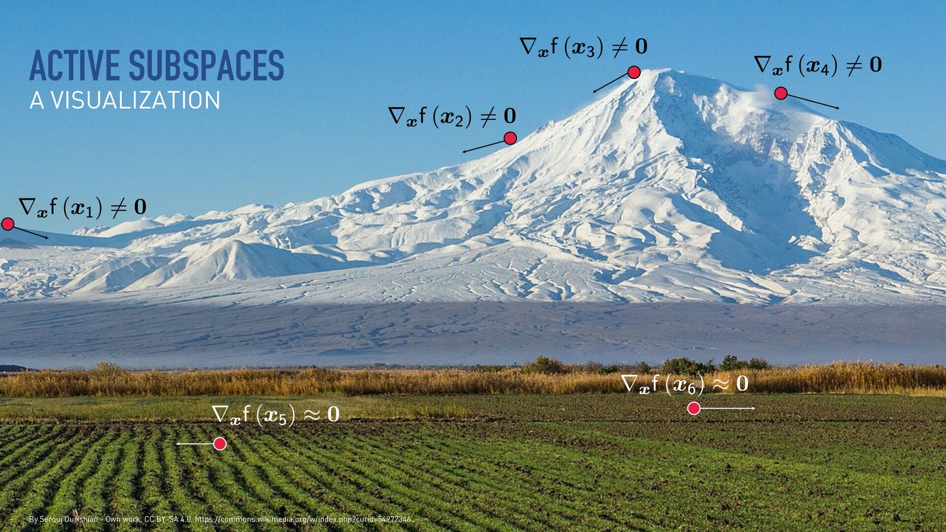
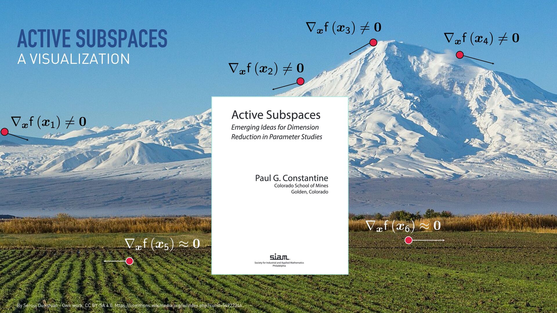
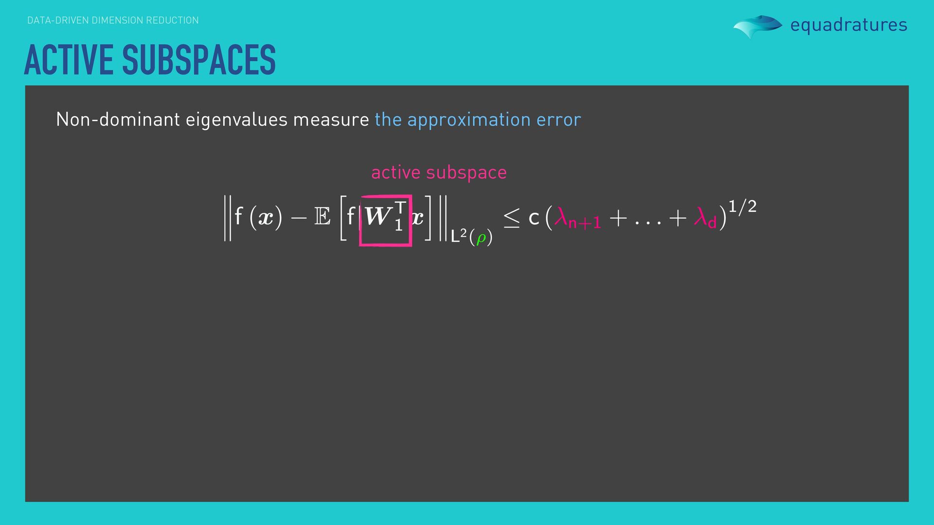
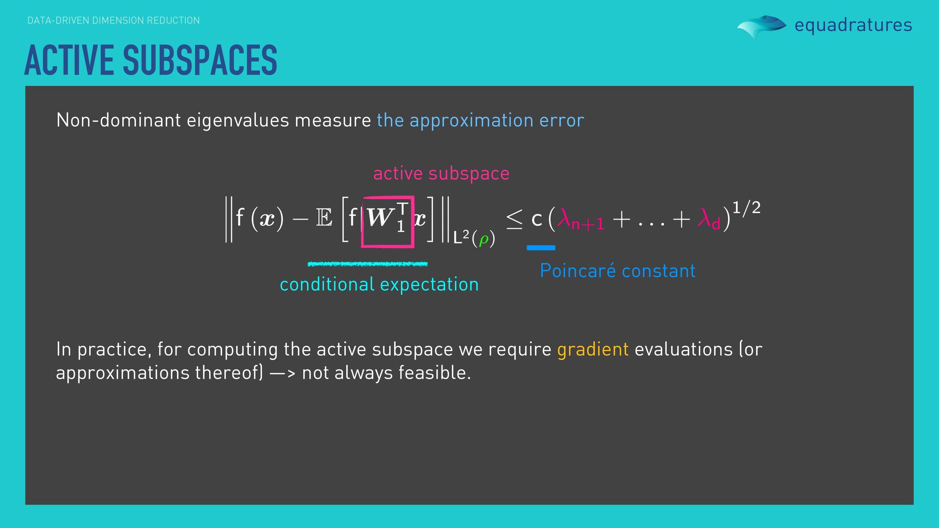
39. DATA-DRIVEN DIMENSION REDUCTION ACTIVE SUBSPACES Non-dominant eigenvalues measure the approximation error conditional expectation active subspace Poincaré constant In practice, for computing the active subspace we require gradient evaluations (or approximations thereof) —> not always feasible.
40. DATA-DRIVEN DIMENSION REDUCTION ACTIVE SUBSPACES Note that active subspaces is NOT principal component analysis (PCA)! aside active subspaces PCA
41. DATA-DRIVEN DIMENSION REDUCTION ACTIVE SUBSPACES This identification of the subspace is important! Consider the following split
42. DATA-DRIVEN DIMENSION REDUCTION ACTIVE SUBSPACES This identification of the subspace is important! Consider the following split
43. DATA-DRIVEN DIMENSION REDUCTION ACTIVE SUBSPACES This identification of the subspace is important! Consider the following split active subpace inactive subpace
44. DATA-DRIVEN DIMENSION REDUCTION ACTIVE SUBSPACES Constructs a quadratic global polynomial model to estimate gradients. from equadratures import * space = Subspaces(method=‘active-subspace’, sample_points=X, sample_outputs=y) CODE
45. DATA-DRIVEN DIMENSION REDUCTION OVERVIEW 1. PRINCIPAL COMPONENTS 2. A SIMPLE EXPERIMENT 3. PROJECTIONS & ZONOTOPES 4. ACTIVE SUBSPACES 5. RIDGE APPROXIMATIONS
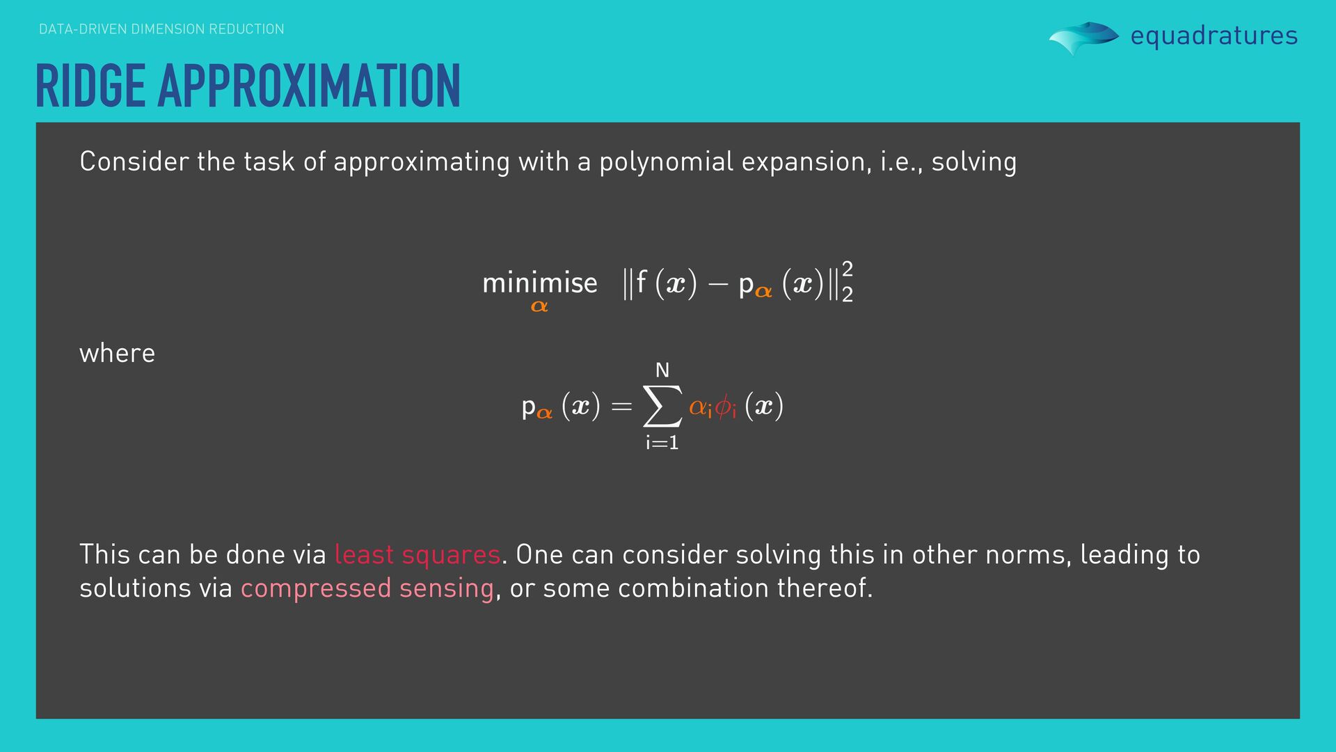
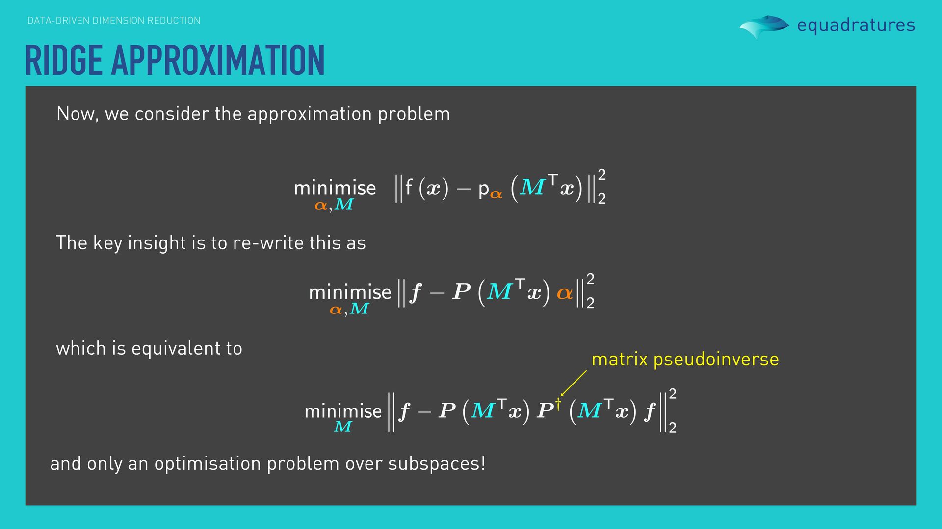
46. DATA-DRIVEN DIMENSION REDUCTION RIDGE APPROXIMATION Consider the task of approximating with a polynomial expansion, i.e., solving This can be done via least squares. One can consider solving this in other norms, leading to solutions via compressed sensing, or some combination thereof. where
47. DATA-DRIVEN DIMENSION REDUCTION RIDGE APPROXIMATION Now, we consider the approximation problem Hokanson & Constantine (2018). SIAM Journal on Scientific Computing. Golub & Pereyra (2003). Inverse Problems.
48. DATA-DRIVEN DIMENSION REDUCTION RIDGE APPROXIMATION Now, we consider the approximation problem The key insight is to re-write this as
49. DATA-DRIVEN DIMENSION REDUCTION RIDGE APPROXIMATION Now, we consider the approximation problem The key insight is to re-write this as which is equivalent to and only an optimisation problem over subspaces! matrix pseudoinverse
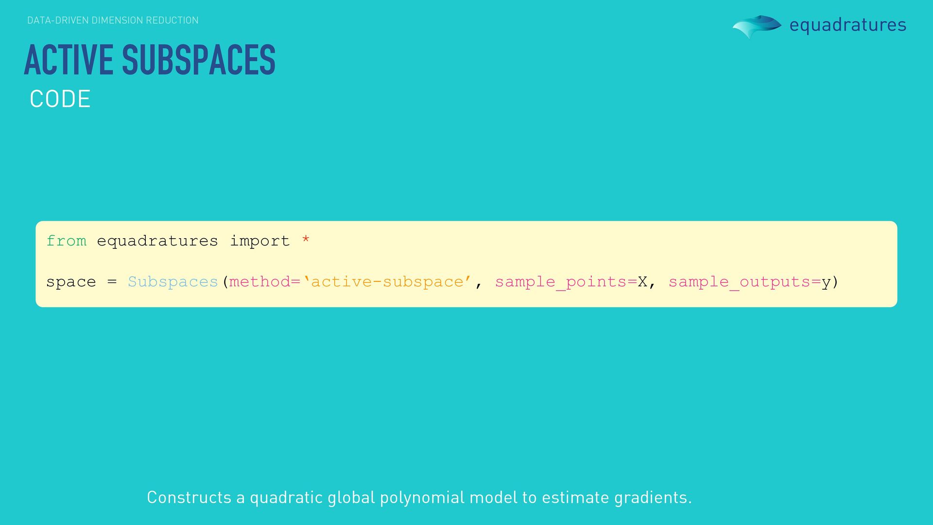
50. DATA-DRIVEN DIMENSION REDUCTION RIDGE APPROXIMATION ridge approximations •Require gradients or gradient estimates (e.g., adjoints). •May require many model evaluations. •The “reduced” dimension is easy to gauge based on eigenvalue decay. active subspaces •Does not require gradients or gradient estimates (e.g., adjoints). •Requires # of model evaluations based on “reduced” dimension. •The “reduced” dimension may need to be estimated.
51. DATA-DRIVEN DIMENSION REDUCTION RIDGE APPROXIMATIONS CODE from equadratures import * space = Subspaces(method=‘variable-projection’, sample_points=X, sample_outputs=y) M = space.get_subspace() subspace_poly = space.get_subspace_polynomial() sobol_indices = subspace_poly().get_sobol_indices() moments = subspace_poly().get_mean_and_variance() space.plot_2D_contour_zonotope()
52. LEARN CONTINUOUS STRUCTURE THANK YOU made by the equadratures team, with ❤