Parametrized Model Checking of Fault Tolerant Distributed Algorithms by Abstraction (part 2)

Igor Konnov, Vienna University of Technology

Transcript

1. Model Checking of Fault-Tolerant Distributed Algorithms Part IV: On the Completeness of Bounded Model Checking: Reachability Igor Konnov Helmut Veith Josef Widder TMPA 2014, Kostroma, Russia
2. Fault-tolerant distributed algorithms n n processes communicate by messages Igor Konnov 2/72
3. Fault-tolerant distributed algorithms n ? ? ? t n processes communicate by messages all processes know that at most t of them might be faulty Igor Konnov 3/72
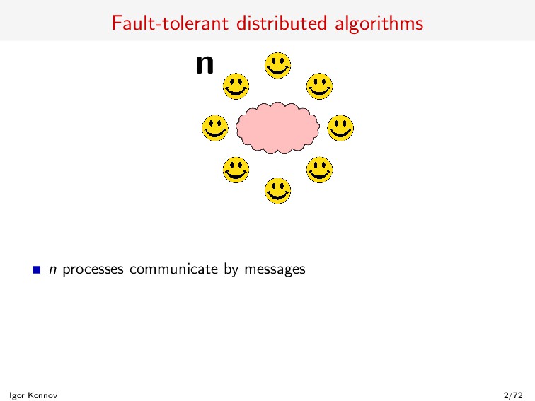
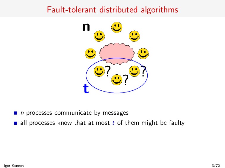
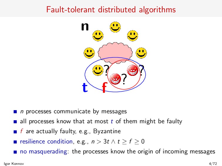
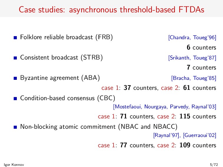
4. Fault-tolerant distributed algorithms n ? ? ? t f n processes communicate by messages all processes know that at most t of them might be faulty f are actually faulty, e.g., Byzantine resilience condition, e.g., n > 3t ∧ t ≥ f ≥ 0 no masquerading: the processes know the origin of incoming messages Igor Konnov 4/72
5. Case studies: asynchronous threshold-based FTDAs Folklore reliable broadcast (FRB) [Chandra, Toueg’96] 6 counters Consistent broadcast (STRB) [Srikanth, Toueg’87] 7 counters Byzantine agreement (ABA) [Bracha, Toueg’85] case 1: 37 counters, case 2: 61 counters Condition-based consensus (CBC) [Mostefaoui, Nourgaya, Parvedy, Raynal’03] case 1: 71 counters, case 2: 115 counters Non-blocking atomic commitment (NBAC and NBACC) [Raynal’97], [Guerraoui’02] case 1: 77 counters, case 2: 109 counters Igor Konnov 5/72
6. Part IV: Outline 1 Yet another abstract model: threshold automata 2 Counter systems with acceleration 3 Parameterized reachability 4 Bounded model checking and its completeness 5 Parameterized bounded model checking and its completeness 6 Main result: diameter of accelerated counter systems (of threshold automata) Igor Konnov 6/72
7. Threshold automata and parameterized reachability Igor Konnov 7/72
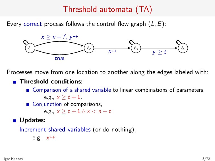
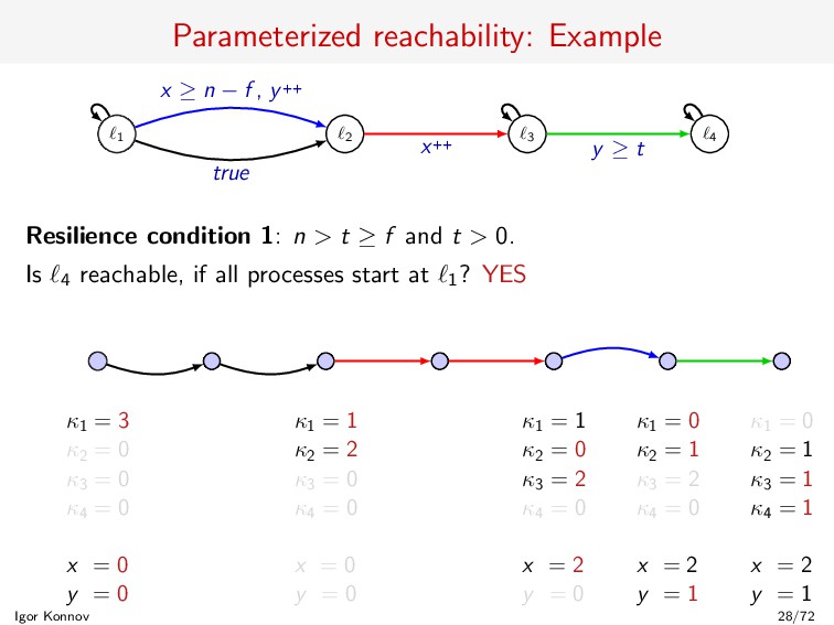
8. Threshold automata (TA) Every correct process follows the control flow graph (L, E): 1 2 3 4 true x ≥ n − f , y++ x++ y ≥ t Processes move from one location to another along the edges labeled with: Threshold conditions: Comparison of a shared variable to linear combinations of parameters, e.g., x ≥ t + 1. Conjunction of comparisons, e.g., x ≥ t + 1 ∧ x < n − t. Updates: Increment shared variables (or do nothing), e.g., x++. Igor Konnov 8/72
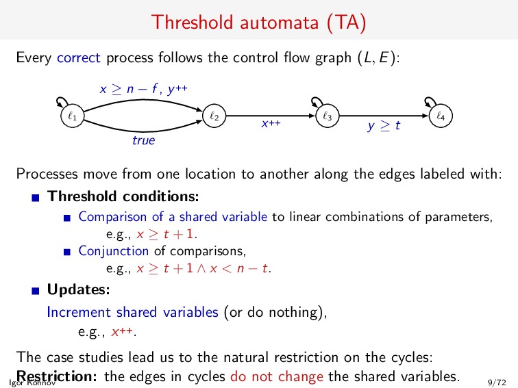
9. Threshold automata (TA) Every correct process follows the control flow graph (L, E): 1 2 3 4 true x ≥ n − f , y++ x++ y ≥ t Processes move from one location to another along the edges labeled with: Threshold conditions: Comparison of a shared variable to linear combinations of parameters, e.g., x ≥ t + 1. Conjunction of comparisons, e.g., x ≥ t + 1 ∧ x < n − t. Updates: Increment shared variables (or do nothing), e.g., x++. The case studies lead us to the natural restriction on the cycles: Restriction: the edges in cycles do not change the shared variables. Igor Konnov 9/72
10. Intuition: threshold automata and threshold-based DAs? 1 2 3 4 true x ≥ n − f , y++ x++ y ≥ t send <x> to all if received <y> from at least t distinct processes Igor Konnov 10/72
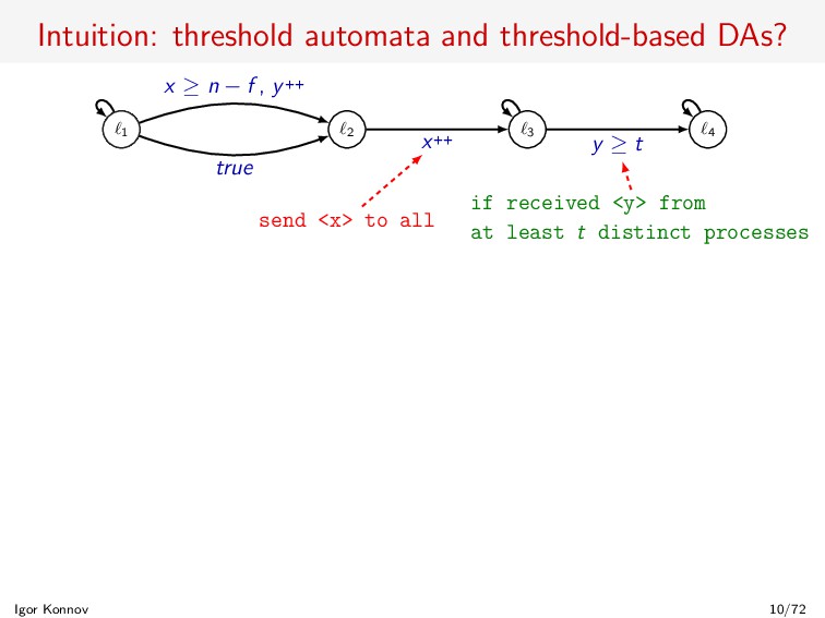
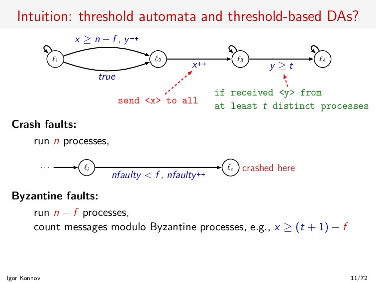
11. Intuition: threshold automata and threshold-based DAs? 1 2 3 4 true x ≥ n − f , y++ x++ y ≥ t send <x> to all if received <y> from at least t distinct processes Crash faults: run n processes, . . . i c crashed here nfaulty < f , nfaulty++ Byzantine faults: run n − f processes, count messages modulo Byzantine processes, e.g., x ≥ (t + 1) − f Igor Konnov 11/72
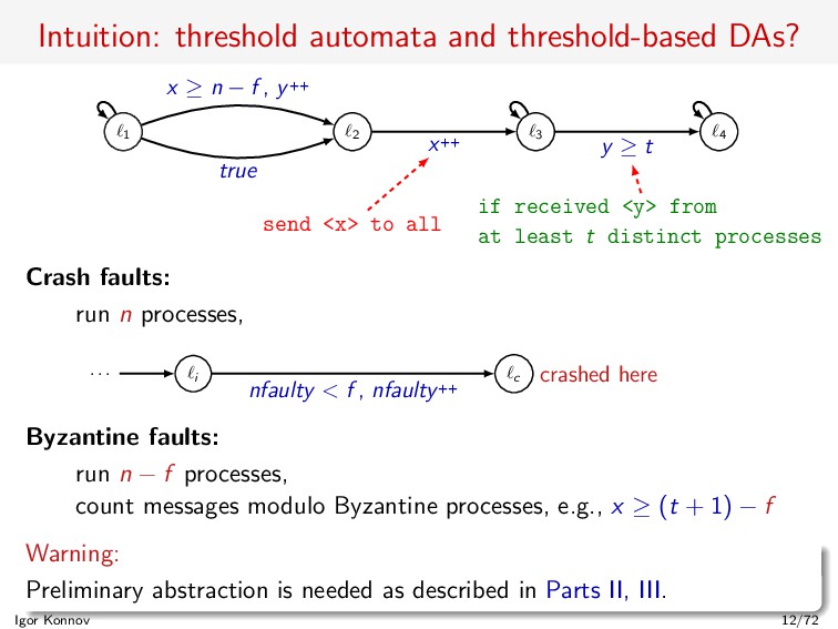
12. Intuition: threshold automata and threshold-based DAs? 1 2 3 4 true x ≥ n − f , y++ x++ y ≥ t send <x> to all if received <y> from at least t distinct processes Crash faults: run n processes, . . . i c crashed here nfaulty < f , nfaulty++ Byzantine faults: run n − f processes, count messages modulo Byzantine processes, e.g., x ≥ (t + 1) − f Warning: Preliminary abstraction is needed as described in Parts II, III. Igor Konnov 12/72
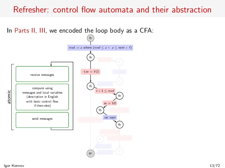
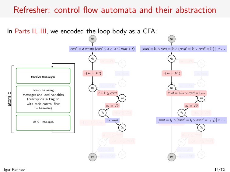
13. Refresher: control flow automata and their abstraction In Parts II, III, we encoded the loop body as a CFA: receive messages compute using messages and local variables (description in English with basic control flow if-then-else) send messages atomic qI q0 q1 q2 q3 sv = V1 ¬(sv = V1) inc nsnt sv := SE q4 q5 q6 q7 q8 qF rcvd := z where (rcvd ≤ z ∧ z ≤ nsnt + f ) ¬(t + 1 ≤ rcvd) t + 1 ≤ rcvd sv = V0 ¬(sv = V0) inc nsnt n − t ≤ rcvd ¬(n − t ≤ rcvd) sv := SE sv := AC Igor Konnov 13/72
14. Refresher: control flow automata and their abstraction In Parts II, III, we encoded the loop body as a CFA: receive messages compute using messages and local variables (description in English with basic control flow if-then-else) send messages atomic qI q0 q1 q2 q3 sv = V1 ¬(sv = V1) inc nsnt sv := SE q4 q5 q6 q7 q8 qF rcvd := z where (rcvd ≤ z ∧ z ≤ nsnt + f ) ¬(t + 1 ≤ rcvd) t + 1 ≤ rcvd sv = V0 ¬(sv = V0) inc nsnt n − t ≤ rcvd ¬(n − t ≤ rcvd) sv := SE sv := AC qI q0 q1 q2 q3 sv = V1 ¬(sv = V1) inc nsnt sv := SE q4 q5 q6 q7 q8 qF rcvd = I0 ∧ nsnt = I0 ∧ (rcvd = I0 ∨ rcvd = I1 ) ∨ . . . ¬(t + 1 ≤ rcvd) rcvd = It+1 ∨ rcvd = In−t sv = V0 ¬(sv = V0) nsnt = I1 ∧ (nsnt = I1 ∨ nsnt = It+1 ) ∨ . . . n − t ≤ rcvd ¬(n − t ≤ rcvd) sv := SE sv := AC Igor Konnov 14/72
15. Intuition: from CFA to TA How to construct TA from CFA? Apply parametric interval abstraction only to the local variables, e.g., rcvd Shared variables, e.g., nsnt, are still unbounded Igor Konnov 15/72
16. Intuition: from CFA to TA How to construct TA from CFA? Apply parametric interval abstraction only to the local variables, e.g., rcvd Shared variables, e.g., nsnt, are still unbounded qI q0 q1 q2 q8 q3 sv = V1 sv = V1 nsnt = nsnt + 1 sv := SE q4 q5 q6 q7 qF nsnt + f ≥ t + 1 ∧ rcvd = In−t ∨ . . . rcvd = I0 ∨ rcvd = I1 rcvd = It+1 ∨ rcvd = In−t sv = V0 nsnt = nsnt + 1 rcvd = In−t sv = AC rcvd = In−t sv = SE sv = V0 Igor Konnov 16/72
17. Intuition: from CFA to TA How to construct TA from CFA? Apply parametric interval abstraction only to the local variables, e.g., rcvd Shared variables, e.g., nsnt, are still unbounded Enumerate all symbolic paths in CFA qI q0 q1 q2 q8 q3 sv = V1 sv = V1 nsnt = nsnt + 1 sv := SE q4 q5 q6 q7 qF nsnt + f ≥ t + 1 ∧ rcvd = In−t ∨ . . . rcvd = I0 ∨ rcvd = I1 rcvd = It+1 ∨ rcvd = In−t sv = V0 nsnt = nsnt + 1 rcvd = In−t sv = AC rcvd = In−t sv = SE sv = V0 Igor Konnov 17/72
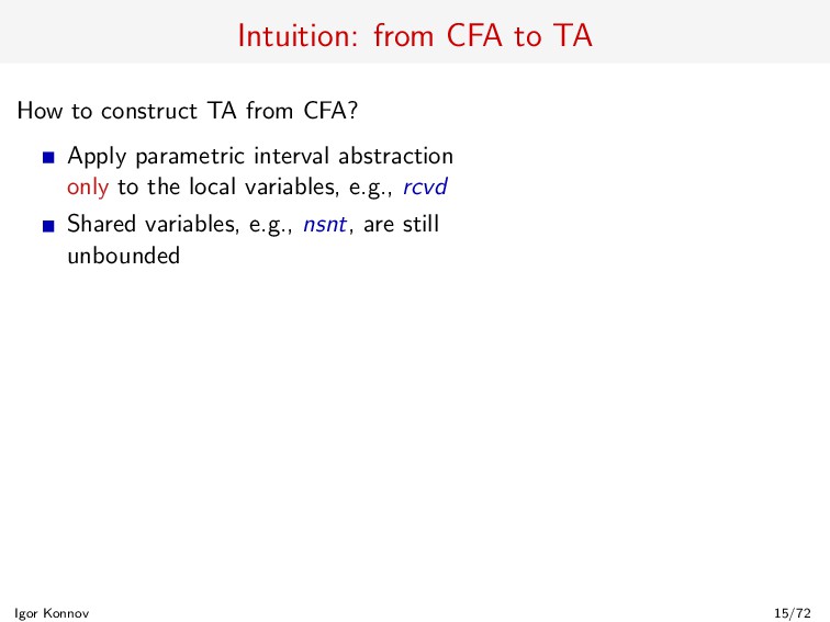
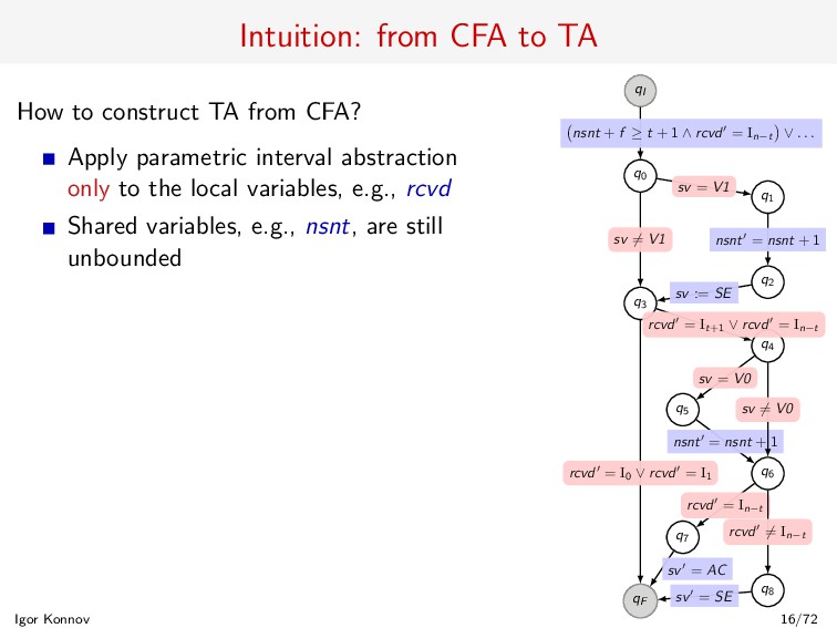
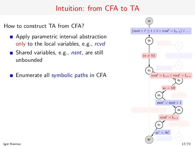
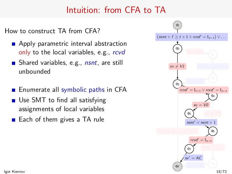
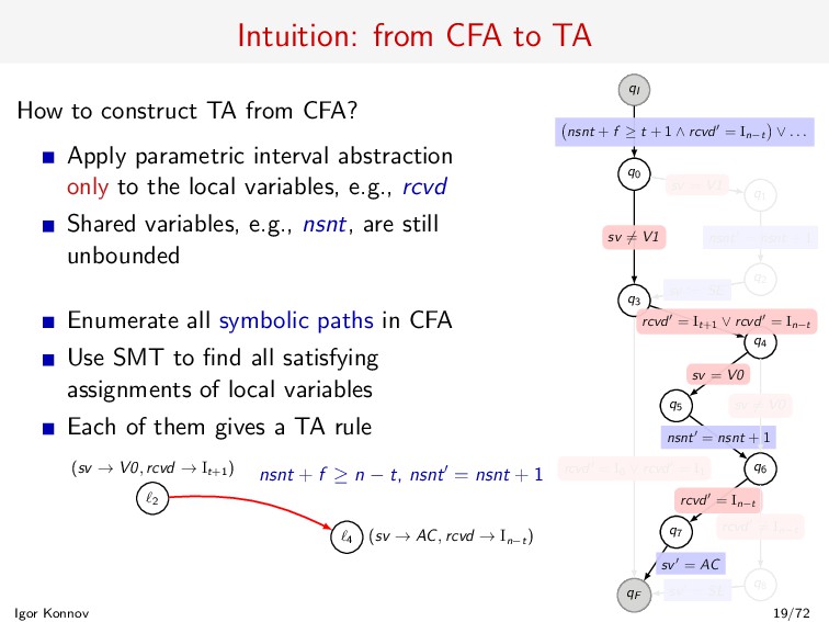
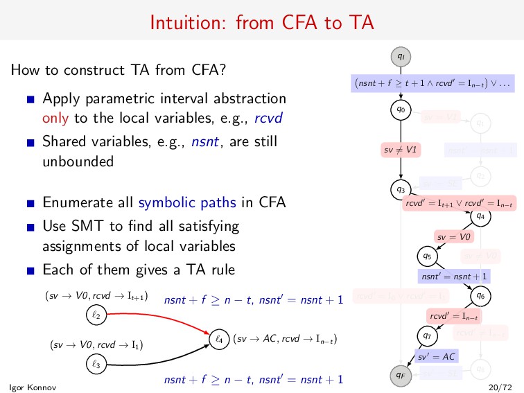
18. Intuition: from CFA to TA How to construct TA from CFA? Apply parametric interval abstraction only to the local variables, e.g., rcvd Shared variables, e.g., nsnt, are still unbounded Enumerate all symbolic paths in CFA Use SMT to find all satisfying assignments of local variables Each of them gives a TA rule qI q0 q1 q2 q8 q3 sv = V1 sv = V1 nsnt = nsnt + 1 sv := SE q4 q5 q6 q7 qF nsnt + f ≥ t + 1 ∧ rcvd = In−t ∨ . . . rcvd = I0 ∨ rcvd = I1 rcvd = It+1 ∨ rcvd = In−t sv = V0 nsnt = nsnt + 1 rcvd = In−t sv = AC rcvd = In−t sv = SE sv = V0 Igor Konnov 18/72
19. Intuition: from CFA to TA How to construct TA from CFA? Apply parametric interval abstraction only to the local variables, e.g., rcvd Shared variables, e.g., nsnt, are still unbounded Enumerate all symbolic paths in CFA Use SMT to find all satisfying assignments of local variables Each of them gives a TA rule 2 (sv → V0, rcvd → It+1 ) 4 (sv → AC, rcvd → In−t ) nsnt + f ≥ n − t, nsnt = nsnt + 1 qI q0 q1 q2 q8 q3 sv = V1 sv = V1 nsnt = nsnt + 1 sv := SE q4 q5 q6 q7 qF nsnt + f ≥ t + 1 ∧ rcvd = In−t ∨ . . . rcvd = I0 ∨ rcvd = I1 rcvd = It+1 ∨ rcvd = In−t sv = V0 nsnt = nsnt + 1 rcvd = In−t sv = AC rcvd = In−t sv = SE sv = V0 Igor Konnov 19/72
20. Intuition: from CFA to TA How to construct TA from CFA? Apply parametric interval abstraction only to the local variables, e.g., rcvd Shared variables, e.g., nsnt, are still unbounded Enumerate all symbolic paths in CFA Use SMT to find all satisfying assignments of local variables Each of them gives a TA rule 2 (sv → V0, rcvd → It+1 ) 4 (sv → AC, rcvd → In−t ) nsnt + f ≥ n − t, nsnt = nsnt + 1 3 (sv → V0, rcvd → I1 ) nsnt + f ≥ n − t, nsnt = nsnt + 1 qI q0 q1 q2 q8 q3 sv = V1 sv = V1 nsnt = nsnt + 1 sv := SE q4 q5 q6 q7 qF nsnt + f ≥ t + 1 ∧ rcvd = In−t ∨ . . . rcvd = I0 ∨ rcvd = I1 rcvd = It+1 ∨ rcvd = In−t sv = V0 nsnt = nsnt + 1 rcvd = In−t sv = AC rcvd = In−t sv = SE sv = V0 Igor Konnov 20/72
21. Threshold Automaton of ST87 (after PIA data abstraction) We automatically summarize process code from Part III: 7 locations, 15 rules (+ self-loops) Guards: black edges: true blue edges: nsnt + f ≥ 1 green edges: nsnt + f ≥ t + 1 red edges: nsnt + f ≥ n − t Actions increment nsnt iff: sv ∈ {v0, v1} to sv ∈ {sent, accept} sv = sent nrcvd = I1 sv = v1 nrcvd = I0 sv = sent nrcvd = I0 sv = v0 nrcvd = I1 sv = sent nrcvd = I2 sv = v0 nrcvd = I0 sv = accept nrcvd = I3 Igor Konnov 21/72
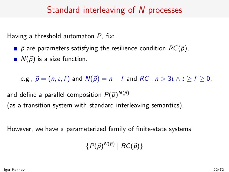
22. Standard interleaving of N processes Having a threshold automaton P, fix: p are parameters satisfying the resilience condition RC(p), N(p) is a size function. e.g., p = (n, t, f ) and N(p) = n − f and RC : n > 3t ∧ t ≥ f ≥ 0. and define a parallel composition P(p)N(p) (as a transition system with standard interleaving semantics). However, we have a parameterized family of finite-state systems: {P(p)N(p) | RC(p)} Igor Konnov 22/72
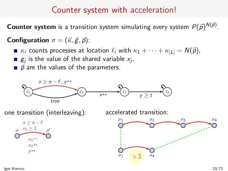
23. Counter system with acceleration! Counter system is a transition system simulating every system P(p)N(p). Configuration σ = (κ, g, p): κi counts processes at location i with κ1 + · · · + κ|L| = N(p), gj is the value of the shared variable xj , p are the values of the parameters. 1 2 3 4 x ≥ n − f , y++ true x++ y ≥ t one transition (interleaving): σ σ x ≥ n − f κ1 ≥ 1 κ1-- κ2++ y++ accelerated transition: σ1 σ2 σ3 σ4 σ1 σ4 ×3 Igor Konnov 23/72
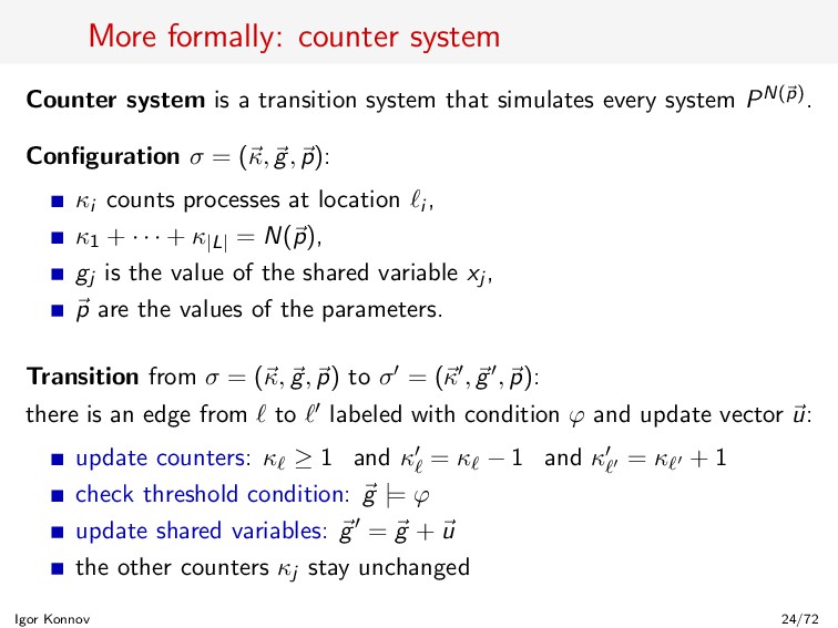
24. More formally: counter system Counter system is a transition system that simulates every system PN(p). Configuration σ = (κ, g, p): κi counts processes at location i , κ1 + · · · + κ|L| = N(p), gj is the value of the shared variable xj , p are the values of the parameters. Transition from σ = (κ, g, p) to σ = (κ , g , p): there is an edge from to labeled with condition ϕ and update vector u: update counters: κ ≥ 1 and κ = κ − 1 and κ = κ + 1 check threshold condition: g |= ϕ update shared variables: g = g + u the other counters κj stay unchanged Igor Konnov 24/72
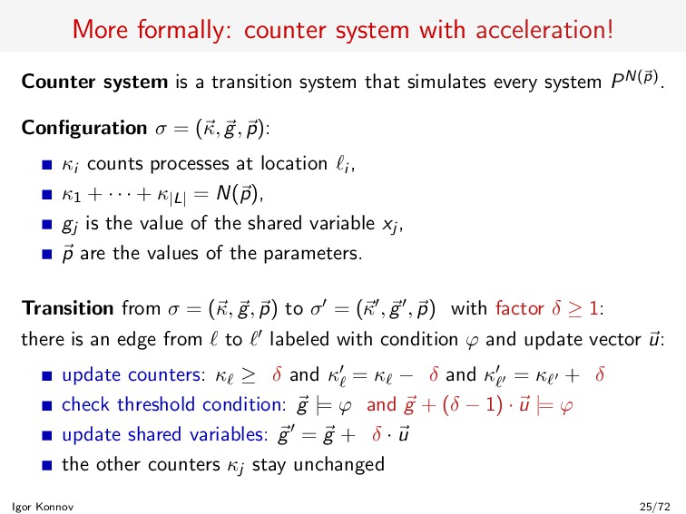
25. More formally: counter system with acceleration! Counter system is a transition system that simulates every system PN(p). Configuration σ = (κ, g, p): κi counts processes at location i , κ1 + · · · + κ|L| = N(p), gj is the value of the shared variable xj , p are the values of the parameters. Transition from σ = (κ, g, p) to σ = (κ , g , p) with factor δ ≥ 1: there is an edge from to labeled with condition ϕ and update vector u: update counters: κ ≥ δ and κ = κ − δ and κ = κ + δ check threshold condition: g |= ϕ and g + (δ − 1) · u |= ϕ update shared variables: g = g + δ · u the other counters κj stay unchanged Igor Konnov 25/72
26. Reachability and parameterized reachability Reachability (fixed parameters): Fix the parameters, e.g., n = 4, t = 1, f = 1, N = n − f = 3. Fix configurations σ and σ of PN. Question: is σ reachable from σ in PN? Igor Konnov 26/72
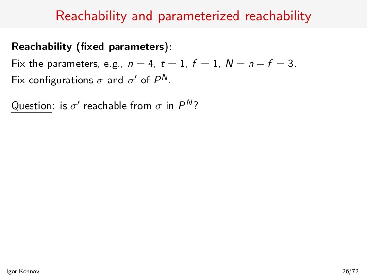
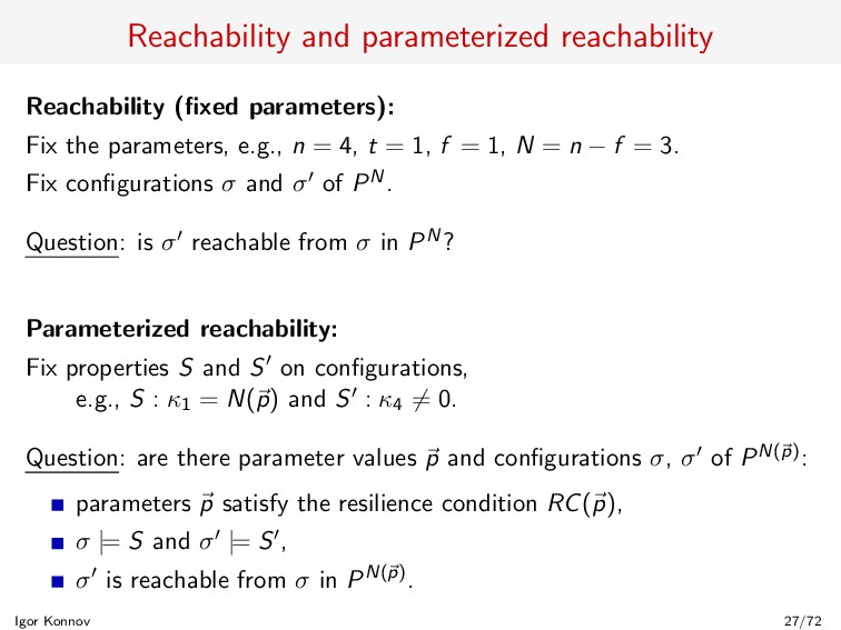
27. Reachability and parameterized reachability Reachability (fixed parameters): Fix the parameters, e.g., n = 4, t = 1, f = 1, N = n − f = 3. Fix configurations σ and σ of PN. Question: is σ reachable from σ in PN? Parameterized reachability: Fix properties S and S on configurations, e.g., S : κ1 = N(p) and S : κ4 = 0. Question: are there parameter values p and configurations σ, σ of PN(p): parameters p satisfy the resilience condition RC(p), σ |= S and σ |= S , σ is reachable from σ in PN(p). Igor Konnov 27/72
28. Parameterized reachability: Example 1 2 3 4 true x ≥ n − f , y++ x++ y ≥ t Resilience condition 1: n > t ≥ f and t > 0. Is 4 reachable, if all processes start at 1? YES κ1 = 3 κ2 = 0 κ3 = 0 κ4 = 0 x = 0 y = 0 κ1 = 1 κ2 = 2 κ3 = 0 κ4 = 0 x = 0 y = 0 κ1 = 1 κ2 = 0 κ3 = 2 κ4 = 0 x = 2 y = 0 κ1 = 0 κ2 = 1 κ3 = 2 κ4 = 0 x = 2 y = 1 κ1 = 0 κ2 = 1 κ3 = 1 κ4 = 1 x = 2 y = 1 Igor Konnov 28/72
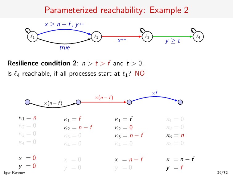
29. Parameterized reachability: Example 2 1 2 3 4 true x ≥ n − f , y++ x++ y ≥ t Resilience condition 2: n > t > f and t > 0. Is 4 reachable, if all processes start at 1? NO κ1 = n κ2 = 0 κ3 = 0 κ4 = 0 x = 0 y = 0 κ1 = f κ2 = n − f κ3 = 0 κ4 = 0 x = 0 y = 0 κ1 = f κ2 = 0 κ3 = n − f κ4 = 0 x = n − f y = 0 κ1 = 0 κ2 = 0 κ3 = n κ4 = 0 x = n − f y = f ×(n − f ) ×(n − f ) ×f Igor Konnov 29/72
30. Parameterized & bounded model checking Igor Konnov 30/72
31. Bounded Model Checking Model checking without BDDs [Biere, Cimatti, Clarke’99] Igor Konnov 31/72
32. Bounded Model Checking Model checking without BDDs [Biere, Cimatti, Clarke’99] Encode as a boolean formula: the transition relation T(x, x ), the set of initial states I(x), the set of bad states B(x). Given a bound k, construct a model checking problem for paths of length k: fk ≡ I(x0) ∧ T(x0, x1) ∧ T(x1, x2) ∧ · · · ∧ T(xk−1, xk) ∧ B(xk) Igor Konnov 32/72
33. Bounded Model Checking Model checking without BDDs [Biere, Cimatti, Clarke’99] Encode as a boolean formula: the transition relation T(x, x ), the set of initial states I(x), the set of bad states B(x). Given a bound k, construct a model checking problem for paths of length k: fk ≡ I(x0) ∧ T(x0, x1) ∧ T(x1, x2) ∧ · · · ∧ T(xk−1, xk) ∧ B(xk) Check fk with a SAT solver. Tools that implement BMC: NuSMV, CBMC, and many other. Igor Konnov 33/72
34. Diameter of a system Consider configurations σ and σ if σ is reachable from σ σ σ Igor Konnov 34/72
35. Diameter of a system Consider configurations σ and σ if σ is reachable from σ then distance dist(σ, σ ) is the length of the shortest path from σ to σ σ σ Igor Konnov 35/72
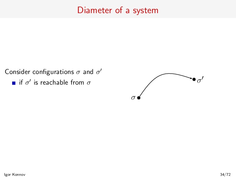
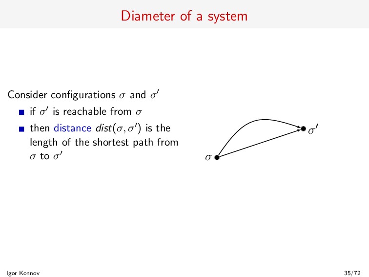
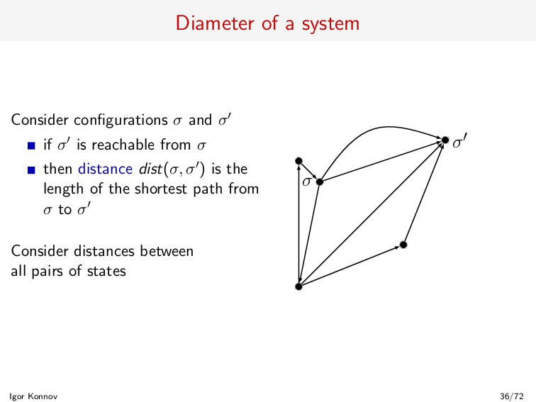
36. Diameter of a system Consider configurations σ and σ if σ is reachable from σ then distance dist(σ, σ ) is the length of the shortest path from σ to σ Consider distances between all pairs of states σ σ Igor Konnov 36/72
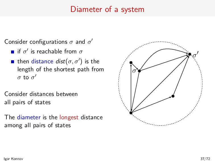
37. Diameter of a system Consider configurations σ and σ if σ is reachable from σ then distance dist(σ, σ ) is the length of the shortest path from σ to σ Consider distances between all pairs of states The diameter is the longest distance among all pairs of states σ σ Igor Konnov 37/72
38. Diameter of a fixed-size system Fix the parameters, e.g., n = 4, t = 1, f = 1. All variables are bounded, the state set is finite. The diameter is bounded by the number of states. n = 4 Igor Konnov 38/72
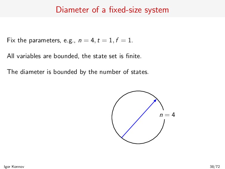
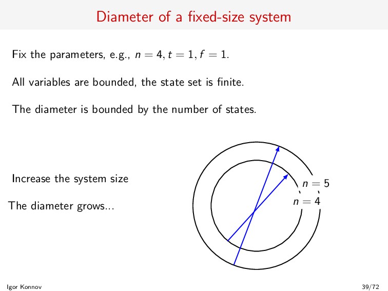
39. Diameter of a fixed-size system Fix the parameters, e.g., n = 4, t = 1, f = 1. All variables are bounded, the state set is finite. The diameter is bounded by the number of states. Increase the system size The diameter grows... n = 4 n = 5 Igor Konnov 39/72
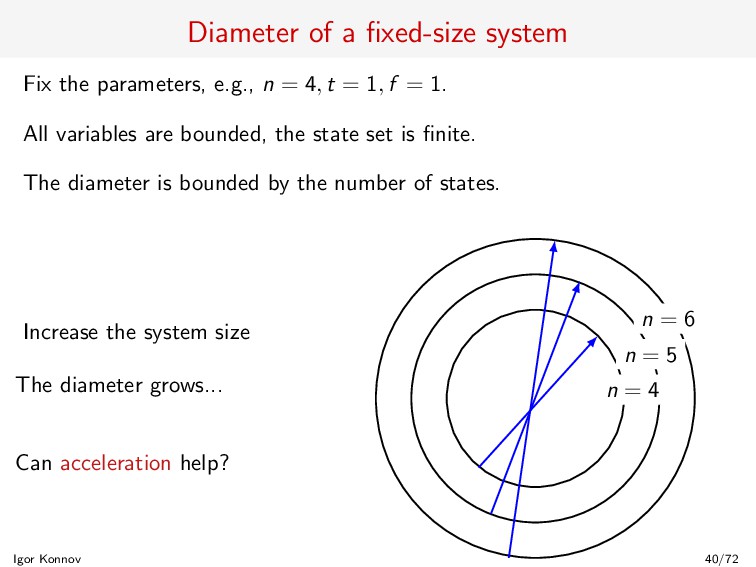
40. Diameter of a fixed-size system Fix the parameters, e.g., n = 4, t = 1, f = 1. All variables are bounded, the state set is finite. The diameter is bounded by the number of states. Increase the system size The diameter grows... Can acceleration help? n = 4 n = 5 n = 6 Igor Konnov 40/72
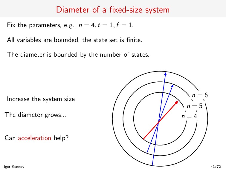
41. Diameter of a fixed-size system Fix the parameters, e.g., n = 4, t = 1, f = 1. All variables are bounded, the state set is finite. The diameter is bounded by the number of states. Increase the system size The diameter grows... Can acceleration help? n = 4 n = 5 n = 6 Igor Konnov 41/72
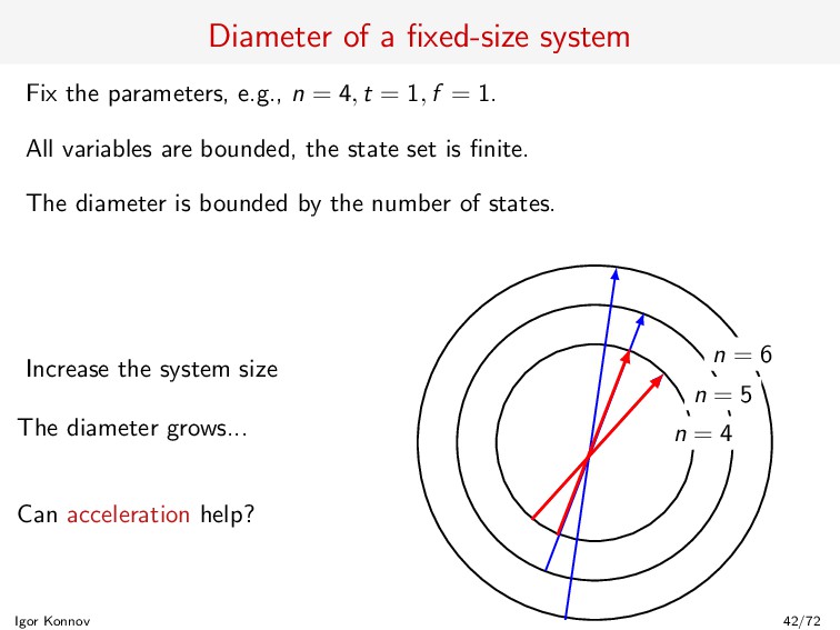
42. Diameter of a fixed-size system Fix the parameters, e.g., n = 4, t = 1, f = 1. All variables are bounded, the state set is finite. The diameter is bounded by the number of states. Increase the system size The diameter grows... Can acceleration help? n = 4 n = 5 n = 6 Igor Konnov 42/72
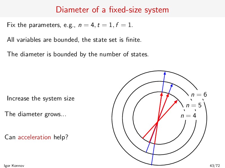
43. Diameter of a fixed-size system Fix the parameters, e.g., n = 4, t = 1, f = 1. All variables are bounded, the state set is finite. The diameter is bounded by the number of states. Increase the system size The diameter grows... Can acceleration help? n = 4 n = 5 n = 6 Igor Konnov 43/72
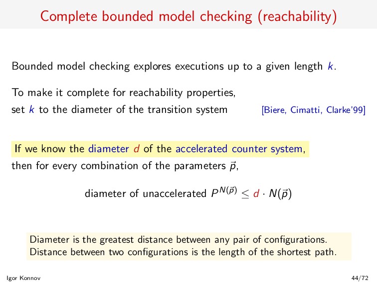
44. Complete bounded model checking (reachability) Bounded model checking explores executions up to a given length k. To make it complete for reachability properties, set k to the diameter of the transition system [Biere, Cimatti, Clarke’99] If we know the diameter d of the accelerated counter system, then for every combination of the parameters p, diameter of unaccelerated PN(p) ≤ d · N(p) Diameter is the greatest distance between any pair of configurations. Distance between two configurations is the length of the shortest path. Igor Konnov 44/72
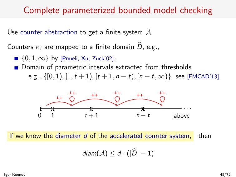
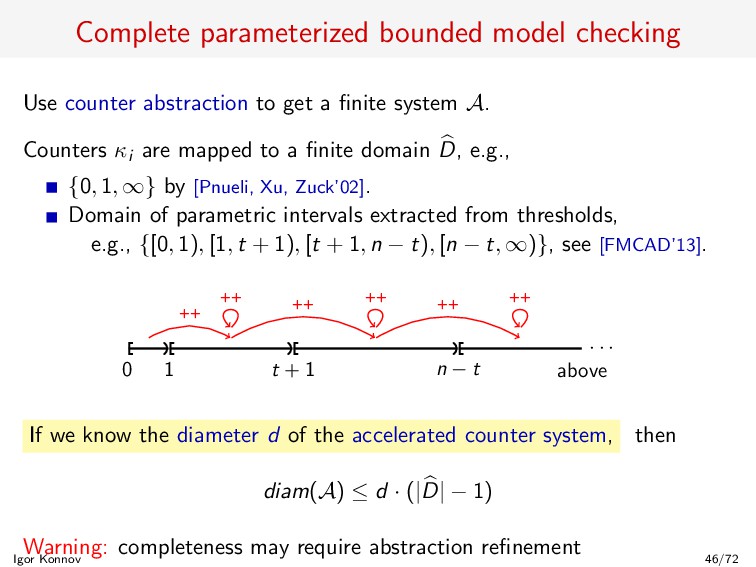
45. Complete parameterized bounded model checking Use counter abstraction to get a finite system A. Counters κi are mapped to a finite domain D, e.g., {0, 1, ∞} by [Pnueli, Xu, Zuck’02]. Domain of parametric intervals extracted from thresholds, e.g., {[0, 1), [1, t + 1), [t + 1, n − t), [n − t, ∞)}, see [FMCAD’13]. 0 1 t + 1 n − t above · · · ++ ++ ++ ++ ++ ++ If we know the diameter d of the accelerated counter system, then diam(A) ≤ d · (|D| − 1) Igor Konnov 45/72
46. Complete parameterized bounded model checking Use counter abstraction to get a finite system A. Counters κi are mapped to a finite domain D, e.g., {0, 1, ∞} by [Pnueli, Xu, Zuck’02]. Domain of parametric intervals extracted from thresholds, e.g., {[0, 1), [1, t + 1), [t + 1, n − t), [n − t, ∞)}, see [FMCAD’13]. 0 1 t + 1 n − t above · · · ++ ++ ++ ++ ++ ++ If we know the diameter d of the accelerated counter system, then diam(A) ≤ d · (|D| − 1) Warning: completeness may require abstraction refinement Igor Konnov 46/72
47. The diameter of the accelerated system? Igor Konnov 47/72
48. Partial orders on TA rules The control flow defines a partial order. Fix a total order lin P ⊆ E × E on the edges (rules): 1 2 3 4 true x ≥ n − f , y++ x++ y ≥ t Igor Konnov 48/72
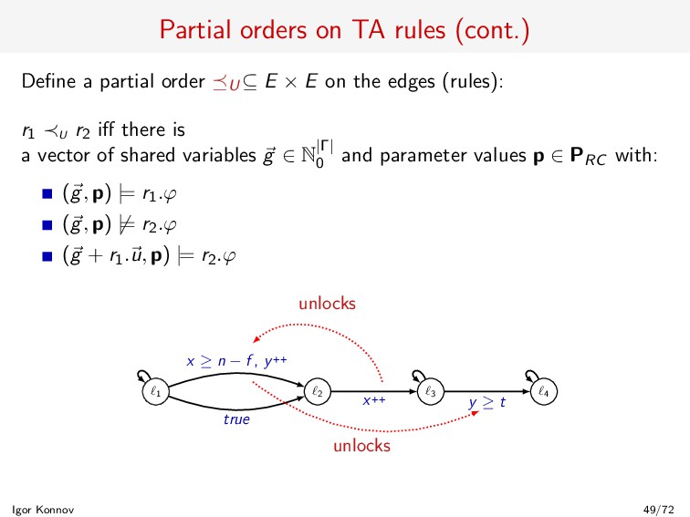
49. Partial orders on TA rules (cont.) Define a partial order U⊆ E × E on the edges (rules): r1 ≺U r2 iff there is a vector of shared variables g ∈ N |Γ| 0 and parameter values p ∈ PRC with: (g, p) |= r1.ϕ (g, p) |= r2.ϕ (g + r1.u, p) |= r2.ϕ 1 2 3 4 true x ≥ n − f , y++ x++ y ≥ t unlocks unlocks Igor Konnov 49/72
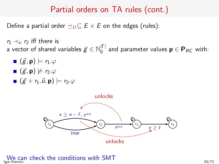
50. Partial orders on TA rules (cont.) Define a partial order U⊆ E × E on the edges (rules): r1 ≺U r2 iff there is a vector of shared variables g ∈ N |Γ| 0 and parameter values p ∈ PRC with: (g, p) |= r1.ϕ (g, p) |= r2.ϕ (g + r1.u, p) |= r2.ϕ 1 2 3 4 true x ≥ n − f , y++ x++ y ≥ t unlocks unlocks We can check the conditions with SMT Igor Konnov 50/72
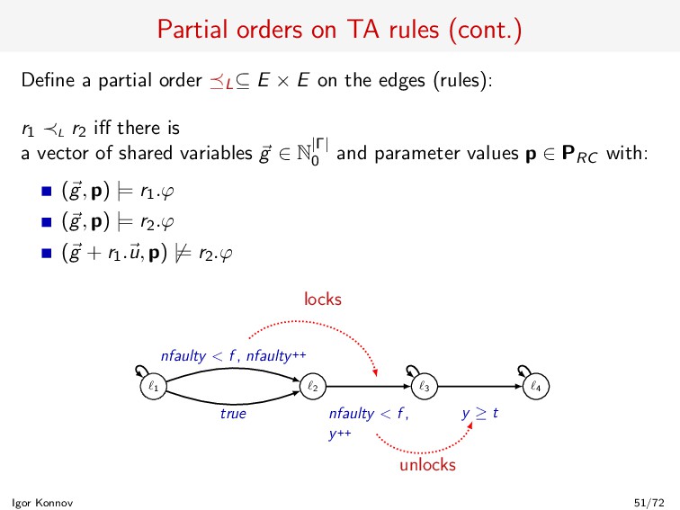
51. Partial orders on TA rules (cont.) Define a partial order L⊆ E × E on the edges (rules): r1 ≺L r2 iff there is a vector of shared variables g ∈ N |Γ| 0 and parameter values p ∈ PRC with: (g, p) |= r1.ϕ (g, p) |= r2.ϕ (g + r1.u, p) |= r2.ϕ 1 2 3 4 true nfaulty < f , nfaulty++ nfaulty < f , y++ y ≥ t locks unlocks Igor Konnov 51/72
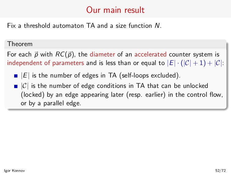
52. Our main result Fix a threshold automaton TA and a size function N. Theorem For each p with RC(p), the diameter of an accelerated counter system is independent of parameters and is less than or equal to |E| · (|C| + 1) + |C|: |E| is the number of edges in TA (self-loops excluded). |C| is the number of edge conditions in TA that can be unlocked (locked) by an edge appearing later (resp. earlier) in the control flow, or by a parallel edge. Igor Konnov 52/72
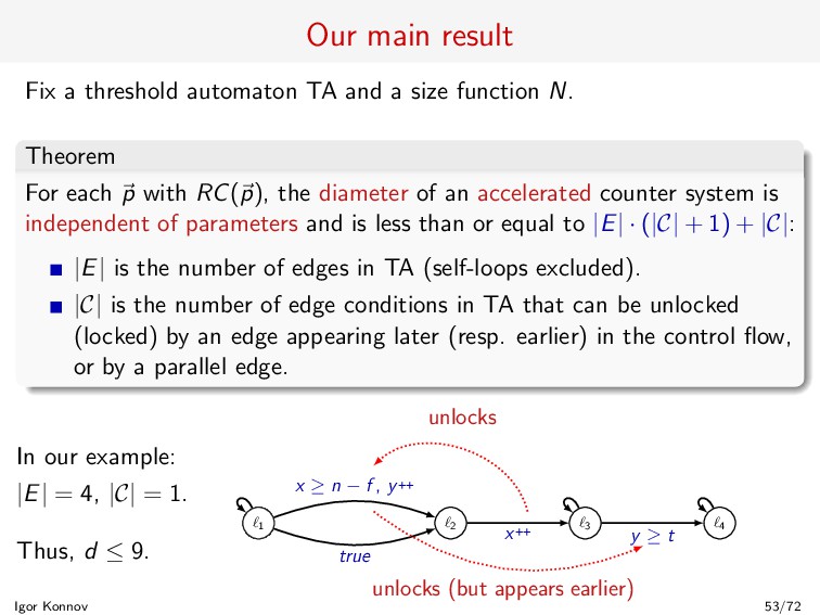
53. Our main result Fix a threshold automaton TA and a size function N. Theorem For each p with RC(p), the diameter of an accelerated counter system is independent of parameters and is less than or equal to |E| · (|C| + 1) + |C|: |E| is the number of edges in TA (self-loops excluded). |C| is the number of edge conditions in TA that can be unlocked (locked) by an edge appearing later (resp. earlier) in the control flow, or by a parallel edge. In our example: |E| = 4, |C| = 1. Thus, d ≤ 9. 1 2 3 4 true x ≥ n − f , y++ x++ y ≥ t unlocks unlocks (but appears earlier) Igor Konnov 53/72
54. Proof idea Igor Konnov 54/72
55. Central idea For each run that connects two configurations we construct a short run by: swapping transitions, and accelerating them Igor Konnov 55/72
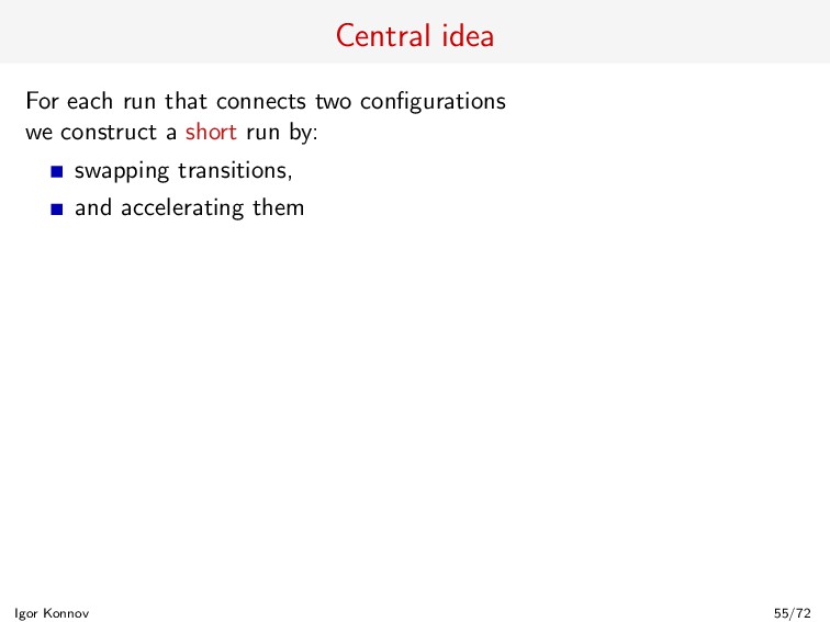
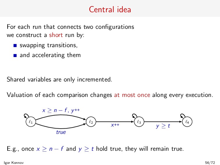
56. Central idea For each run that connects two configurations we construct a short run by: swapping transitions, and accelerating them Shared variables are only incremented. Valuation of each comparison changes at most once along every execution. 1 2 3 4 true x ≥ n − f , y++ x++ y ≥ t E.g., once x ≥ n − f and y ≥ t hold true, they will remain true. Igor Konnov 56/72
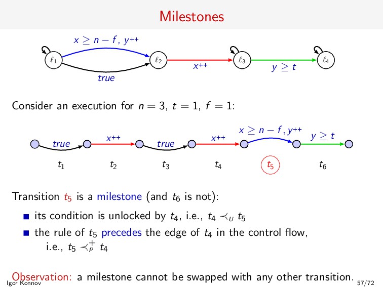
57. Milestones 1 2 3 4 true x ≥ n − f , y++ x++ y ≥ t Consider an execution for n = 3, t = 1, f = 1: true true x++ x++ x ≥ n − f , y++ y ≥ t t1 t2 t3 t4 t5 t6 Transition t5 is a milestone (and t6 is not): its condition is unlocked by t4, i.e., t4 ≺U t5 the rule of t5 precedes the edge of t4 in the control flow, i.e., t5 ≺+ P t4 Observation: a milestone cannot be swapped with any other transition. Igor Konnov 57/72
58. Sorting the transitions (with acyclic control flow) 1 2 3 4 true x ≥ n − f , y++ x++ y ≥ t Igor Konnov 58/72
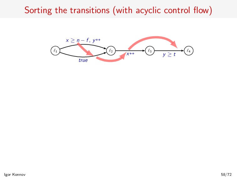
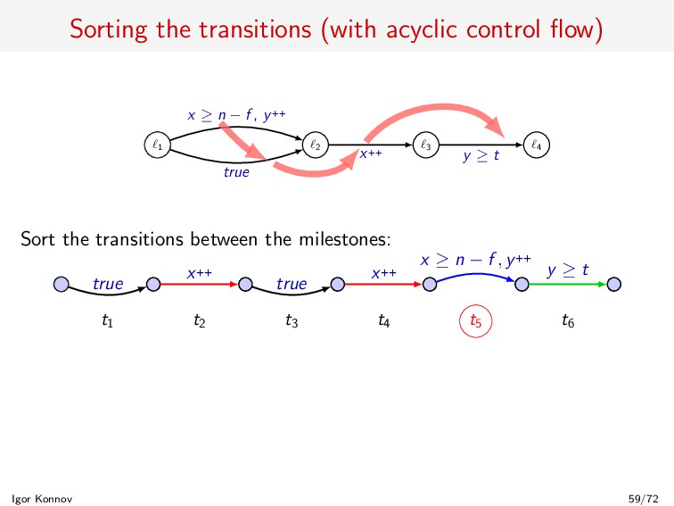
59. Sorting the transitions (with acyclic control flow) 1 2 3 4 true x ≥ n − f , y++ x++ y ≥ t Sort the transitions between the milestones: true true x++ x++ x ≥ n − f , y++ y ≥ t t1 t2 t3 t4 t5 t6 Igor Konnov 59/72
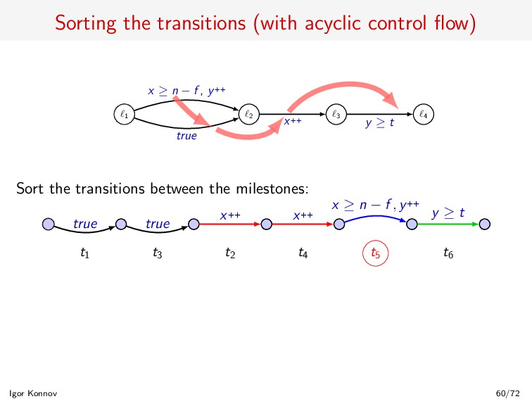
60. Sorting the transitions (with acyclic control flow) 1 2 3 4 true x ≥ n − f , y++ x++ y ≥ t Sort the transitions between the milestones: true true x++ x++ x ≥ n − f , y++ y ≥ t t1 t3 t2 t4 t5 t6 Igor Konnov 60/72
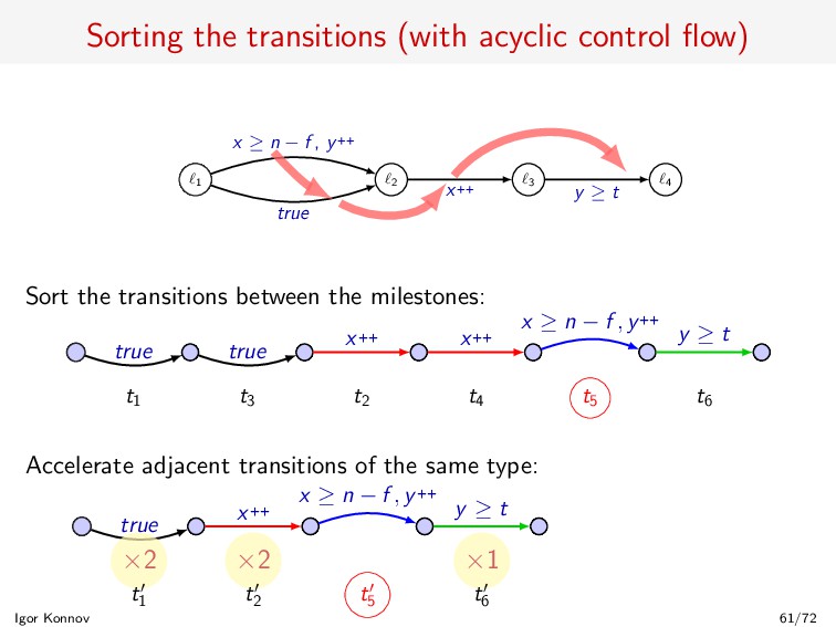
61. Sorting the transitions (with acyclic control flow) 1 2 3 4 true x ≥ n − f , y++ x++ y ≥ t Sort the transitions between the milestones: true true x++ x++ x ≥ n − f , y++ y ≥ t t1 t3 t2 t4 t5 t6 Accelerate adjacent transitions of the same type: true x++ x ≥ n − f , y++ y ≥ t ×2 ×2 ×1 t1 t2 t5 t6 Igor Konnov 61/72
62. How long is an accelerated execution? The number of milestones is bounded with |C|: the number of edge conditions that can be unlocked (locked) by an edge appearing later (resp. earlier) in the control flow, or by a parallel edge. The length of each segment (sorted and accelerated) is bounded with |E|: the number of edges in the threshold automaton The length of an accelerated execution is bounded with: |E| length of each segment × (|C| + 1) number of segments + |C| number of milestones So is the diameter of the accelerated counter system. Igor Konnov 62/72
63. Evaluation Igor Konnov 63/72
64. Case studies: asynchronous threshold-based FTDAs Toy example (Toy) [we made it up] 5 locations, 8 rules Folklore reliable broadcast (FRB) [Chandra, Toueg’96] 6 locations, 15 rules Consistent broadcast (STRB) [Srikanth, Toueg’87] 7 locations, 21 rule Byzantine agreement (ABA) [Bracha, Toueg’85] case 1: 37 counters, 202 rules; case 2: 61 locations, 425 rules Condition-based consensus (CBC) [Mostefaoui, Nourgaya, Parvedy, Raynal’03] case 1: 71 counter, 408 rules; case 2: 115 counters and 991 rule Non-blocking atomic commitment (NBAC and NBACC) [Raynal’97], [Guerraoui’02] case 1: 77 counters, 1356 rules; case 2: 109 counters, 1831 rule Igor Konnov 64/72
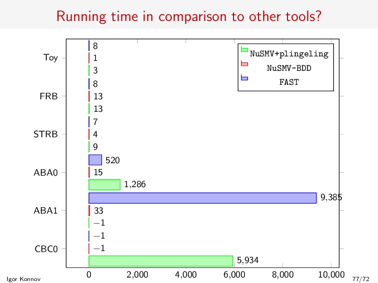
65. Implementation We encode the distributed algorithms in parameteric Promela Our tool ByMC implements counter abstraction/refinement loop NuSMV does bounded model checking of the counter abstraction: either with MiniSAT, or Plingeling (multicore SAT solver) Everything is available at: http://forsyte.at/software/bymc Igor Konnov 65/72
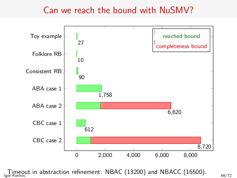
66. Can we reach the bound with NuSMV? 0 2,000 4,000 6,000 8,000 Toy example Folklore RB Consistent RB ABA case 1 ABA case 2 CBC case 1 CBC case 2 27 10 90 1,758 6,620 612 8,720 reached bound completeness bound Timeout in abstraction refinement: NBAC (13200) and NBACC (16500). Igor Konnov 66/72
67. Conclusions for Part IV Polynomial bound on the diameter of accelerated counter systems (for threshold automata) Our results allow us to use bounded model checking as a complete method for reachability in systems of threshold automata of: a fixed size, a parameterized size Igor Konnov 67/72
68. Conclusions for Part IV Polynomial bound on the diameter of accelerated counter systems (for threshold automata) Our results allow us to use bounded model checking as a complete method for reachability in systems of threshold automata of: a fixed size, a parameterized size Bounds for liveness properties? Better implementation? Igor Konnov 68/72
69. Our current work Discrete synchronous Discrete partially synchronous Discrete asynchronous Continuous synchronous Continuous partially synchronous One instance/ finite payload Many inst./ finite payload Many inst./ unbounded payload Messages with reals core of {ST87, BT87, CT96}, MA06 (common), MR04 (binary) one-shot broadcast, c.b.consensus Igor Konnov 69/72
70. Future work: threshold guards + orthogonal features Discrete synchronous Discrete partially synchronous Discrete asynchronous Continuous synchronous Continuous partially synchronous One instance/ finite payload Many inst./ finite payload Many inst./ unbounded payload Messages with reals core of {ST87, BT87, CT96}, MA06 (common), MR04 (binary) one-shot broadcast, c.b.consensus DHM12 ST87 AK00 CT96 (failure detector) DLS86, MA06, L98 (Paxos) ST87, BT87, CT96, DAs with failure-detectors DLPSW86 DFLPS13 WS07 ST87 (JACM) FSFK06 WS09 clock sync broadcast approx. agreement Igor Konnov 70/72
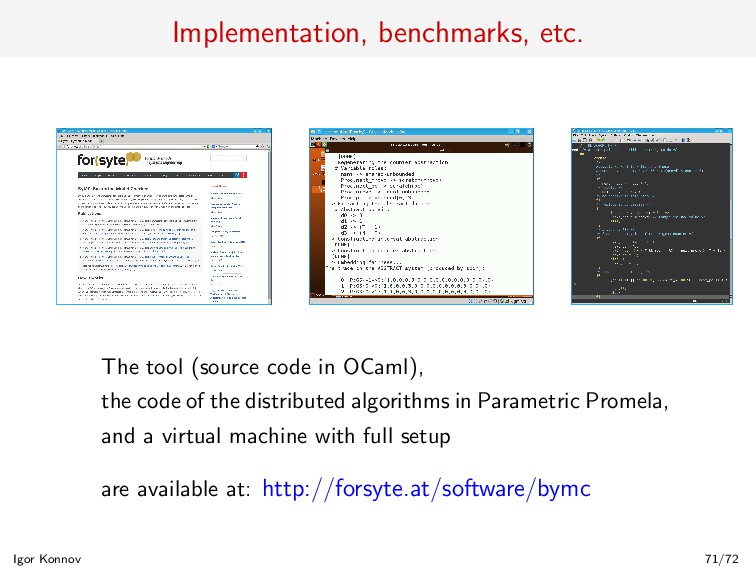
71. Implementation, benchmarks, etc. The tool (source code in OCaml), the code of the distributed algorithms in Parametric Promela, and a virtual machine with full setup are available at: http://forsyte.at/software/bymc Igor Konnov 71/72
72. Thank you! http://forsyte.at/software/bymc Doctoral College: Vienna, Graz, Linz http://logic-cs.at Igor Konnov 72/72
73. Dealing with cycles: the idea Recall that cycles do not update shared variables. Find strongly connected components in the control flow graph and define equivalence classes of edges. When sorting the segments, preserve the relative order of transitions within the equivalence classes. After sorting, remove the cycles. The length of an acyclic accelerated execution is bounded as before. Igor Konnov 73/72
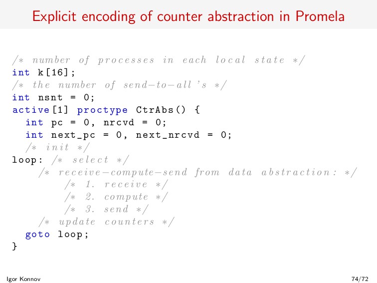
74. Explicit encoding of counter abstraction in Promela /∗ number of p r o c e s s e s in each l o c a l s t a t e ∗/ int k[16]; /∗ the number of send−to−a l l ’ s ∗/ int nsnt = 0; active [1] proctype CtrAbs () { int pc = 0, nrcvd = 0; int next_pc = 0, next_nrcvd = 0; /∗ i n i t ∗/ loop: /∗ s e l e c t ∗/ /∗ r e c e i v e −compute−send from data a b s t r a c t i o n : ∗/ /∗ 1. r e c e i v e ∗/ /∗ 2. compute ∗/ /∗ 3. send ∗/ /∗ update count e rs ∗/ goto loop; } Igor Konnov 74/72
75. Diameters of counter systems Our bound on the diameter of an (accelerated) counter system of a threshold automaton is |E| · (|C| + 1) + |C|, or O(|E|2). The number of conditions |C| is usually small, so we can bound the diameter with O(|E|). Igor Konnov 75/72
76. Forklore Reliable Broadcast crash faults, regular model checking for FTDA [Fisman, Kupferman, Lustig 2008], our technique also works with I0 = [0; 1) and I1 = [1; ∞). qI q1 q2 q3 q4 q5 qF rcvd ≤ rcvd ∧ rcvd ≤ nsnt + nsntf sv = V1 sv = V0 sv = AC sv = CR 1 > rcvd 1 ≤ rcvd sv = CR nsntf = nsntf + 1 sv = AC nsnt = nsnt + 1 Igor Konnov 76/72
77. Running time in comparison to other tools? 0 2,000 4,000 6,000 8,000 10,000 Toy FRB STRB ABA0 ABA1 CBC0 3 13 9 1,286 −1 5,934 1 13 4 15 33 −1 8 8 7 520 9,385 −1 NuSMV+plingeling NuSMV-BDD FAST Igor Konnov 77/72
78. The diameter and refinement The diameter does not grow up in the course of refinement! Igor Konnov 78/72
79. Petri nets? Igor Konnov 79/72