Upgrade to Pro — share decks privately, control downloads, hide ads and more …

Automated acquisition of explainable knowledge from unannotated histopathology images

harunashi
July 02, 2021

Automated acquisition of explainable knowledge from unannotated histopathology images

harunashi

July 02, 2021
Tweet

More Decks by harunashi

Other Decks in Science

Transcript

  1. Automated acquisition
    of explainable
    knowledge from
    unannotated
    histopathology images
    7/2 (⾦) MERC

    View Slide

  2. お品書き
    • Abstract
    • Introduction
    • Method
    • Result
    • おまけ:オートエンコーダーで教師なし分類実装

    View Slide

  3. Abstract
    • アノテーションなしの教師なし学習で前⽴腺癌の再発を予測
    • オートエンコーダーで特徴抽出してSVM
    • 5年後再発予測がAUC=0.84

    View Slide

  4. Introduction
    • 欧⽶⼈に多い、50歳以上男性に好発する
    • 病期、癌の悪性度(グリーソンスコア)、PSA値から治療⽅針を
    決定
    • 前⽴腺内にとどまるなら根治的前⽴腺摘除術で治療
    • 術後再発が問題になる(追加で薬剤を使うか??)
    前⽴腺癌 prostatic carcinoma

    View Slide

  5. Introduction
    • グリーソンスコア
    • 多くの⾯積を占める順に第⼀パターン、
    第⼆パターンを決定、その合計がスコア
    • 6以下で予後良好、8以上で不良
    • 予後とよく相関する
    病気がみえるvol.8 腎・泌尿器

    View Slide

  6. 補⾜
    • オートエンコーダー:⾃⼰符号器
    ⼊⼒
    出⼒
    ⼊⼒と同じ出⼒を⾏うニューラルネットワーク
    中間層が少なくなっている
    少ない情報から元の情報を復元する
    →中間層に特徴が抽出されていると考えられる

    View Slide

  7. Method
    • 根治的前⽴腺摘除術を受けた患者の1年以内、5年以内の再発
    を予測する
    • 再発=BCR(⽣化学的再発)
    PSA値が0.2ng/mL以上に上昇した場合、再発。
    • ⽇本医科⼤学付属病院のデータで訓練
    聖マリアンナ医科⼤学病院(SMH)と愛知医科⼤学病院
    (AMH)で外部検証

    View Slide

  8. Method
    • 予測の⽅法 ざっくり。

    View Slide

  9. Examples of compressed images.

    View Slide

  10. Method
    病理画像 100個の特徴量
    Lasso
    Ridge
    SVM
    病理画像 グリソンスコア
    オートエンコーダー
    k-means
    専⾨医

    View Slide

  11. Data
    Data
    • 訓練データ
    ⽇本医科⼤学付属病院(NMSH)
    842例の病理画像セット
    • 外部検証
    聖マリアンナ医科⼤学病院(SMH)と愛知医科⼤学病院(AMH)
    95例の病理画像セット

    View Slide

  12. Data
    Data
    • 訓練データ
    100⼈×100枚の病理画像→オートエンコーダーの訓練
    残りの742⼈→抽出した特徴量を使って予測の訓練
    • ひとつの画像の画素数は平均1億4千万
    →モデルの学習には約960億枚に相当

    View Slide

  13. Key feature generation method
    • でっかいサイズの病理画像を100個の特徴量まで圧縮したい
    • STEP1 弱拡⼤の画像に対して
    • STEP2 強拡⼤の画像に対して
    • STEP3 STEP1で得た結果をSTEP2の結果と⽐較して補完
    →100個の特徴量を得る

    View Slide

  14. Key feature generation method

    View Slide

  15. Key feature generation method

    View Slide

  16. Key feature generation method
    ui,j,k
    Si,j
    のk番⽬の特徴に対するスコア
    di,j.k
    Si,j
    のk番⽬のセントロイドとの距離
    ⼩画像ごとに2048個の特徴データが得られる

    View Slide

  17. Key feature generation method

    View Slide

  18. Key feature generation method
    score 100 clusters using the ratio of the number of positive/negative images
    based on the similarity to each cluster.
    k番⽬のクラスタが再発に働くのか⾮再発に働くのか
    の程度のスコアを付ける。

    View Slide

  19. Key feature generation method
    • 100種類ある特徴にはそれぞれ再発に働く度合いが
    スコアとして与えられている。
    ex. 特徴28はスコア0.76→再発に働く
    特徴60はスコア0.47→⾮再発に働く
    • ⼩画像 Si,j
    に対して100個ある特徴のうち1つが与えられる
    • 画像Si
    は100個の特徴を持つ

    View Slide

  20. Key feature generation method

    View Slide

  21. View Slide

  22. Key feature generation method
    STEP2はSTEP1の結果を補完する

    View Slide

  23. Key feature generation method
    ←The 1568 intermediate-layer features were
    given scores uʼi,j,jʼ,kʼ
    based on the intensity values
    vʼi,j,jʼ
    of each node. Again, we used the following
    simple scoring method:

    View Slide

  24. Key feature generation method
    • STEP3
    • 各⼩画像は
    STEP1の特徴kについてのIi,j

    STEP2の特徴kʼについての Iʼi,j
    を持つ。
    • Ii,j
    , Iʼi,j
    を0.5を閾値としてposi,negaとし、⼀致しない場合は
    解析に使わない
    • STEP1で得た特徴量の数を合計して予測に⽤いた。

    View Slide

  25. Result
    Data
    • 訓練データ
    ⽇本医科⼤学付属病院(NMSH)
    842例の病理画像セット
    • 外部検証
    聖マリアンナ医科⼤学病院(SMH)と愛知医科⼤学病院(AMH)
    95例の病理画像セット

    View Slide

  26. Result
    Data
    • 訓練データ
    100⼈×100枚の病理画像→オートエンコーダーの訓練
    残りの742⼈→抽出した特徴量を使って予測の訓練
    • ひとつの画像の画素数は平均1億4千万
    →モデルの学習には約960億枚に相当

    View Slide

  27. Result
    1年以内再発予測
    SVMで0.82
    SVM+Gleasonで0.84

    View Slide

  28. Result
    1年以内再発予測

    View Slide

  29. Result
    5年以内再発予測

    View Slide

  30. Result
    外部検証

    View Slide

  31. Explainable features from
    histopathology images
    • k-meansで得られる100個のセントロイド
    →100個の特徴、
    セントロイドに最も近い画像が特徴を代表する画像
    • 各特徴(セントロイド)が悪性なのか、良性なのかは再発データ
    に基づいてスコアがつけられている
    • 代表する画像を病理医が⾒て意味を解釈する

    View Slide

  32. Explainable features from
    histopathology images
    • a-j 異常な構造
    • c 
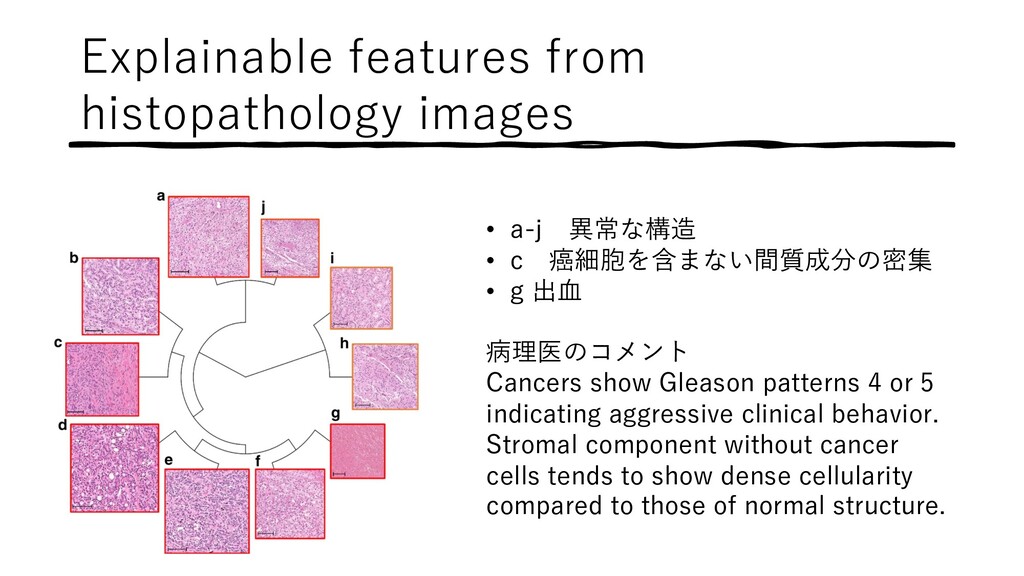
癌細胞を含まない間質成分の密集
    • g 出⾎
    病理医のコメント
    Cancers show Gleason patterns 4 or 5
    indicating aggressive clinical behavior.
    Stromal component without cancer
    cells tends to show dense cellularity
    compared to those of normal structure.

    View Slide

  33. Explainable features from
    histopathology images
    • p グリソンスコア3に相当
    • k-o, 
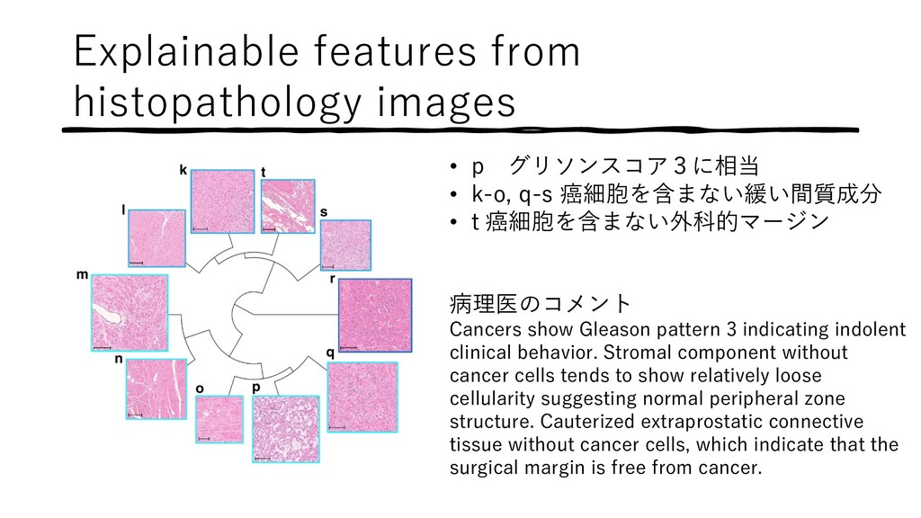
q-s 癌細胞を含まない緩い間質成分
    • t 癌細胞を含まない外科的マージン
    病理医のコメント
    Cancers show Gleason pattern 3 indicating indolent
    clinical behavior. Stromal component without
    cancer cells tends to show relatively loose
    cellularity suggesting normal peripheral zone
    structure. Cauterized extraprostatic connective
    tissue without cancer cells, which indicate that the
    surgical margin is free from cancer.

    View Slide

  34. Discussion
    • The Gleason score is a unique pathological grading system,
    purely based on architectural disorders, without
    considering cytological atypia. In this study, none of the
    cancer cells in the images identified by the deep neural
    networks as representative of high-grade cancer showed
    severe nuclear atypia or prominent nucleoli. Our results
    indicate that the central ideas behind Gleasonʼs grading
    system are sound.

    View Slide

  35. Discussion
    • Interestingly, representative images of the features
    nominated by the deep neural networks comprised of not
    only human-established findings but also previously
    unspotlighted or neglected features of stroma at the
    noncancerous area.

    View Slide

  36. おまけ
    教師なしで画像を分類してみたい。
    1. オートエンコーダーを作る
    2. 中間層の出⼒を取り出す
    3. 出⼒をもとにしてSVMで分類をする
    4. 中間層の出⼒を次元圧縮して分布を⾒る(特徴抽出できてい
    るか?)

    View Slide

  37. おまけ
    • データはMNISTの「1」と「8」だけ、28*28
    • 畳み込みではなく全結合
    • ホントはk-meansのセントロイドとの距離を特徴量にして
    次元削減してからSVMしたかったけどめんどくさいので断念

    View Slide

  38. おまけ
    • オートエンコーダー
    28×28→36次元、⼀層の単純なニューラルネットワーク

    View Slide

  39. おまけ
    • オートエンコーダー出⼒を⾒る
    若⼲滲むが良い感じ。

    View Slide

  40. おまけ
    • 中間層の出⼒を得る
    出⼒層を削除してエンコーダーとして保存
    中間層の出⼒を並べてみる

    View Slide

  41. おまけ
    • 得た中間層の出⼒は36次元
    PCAで2次元に圧縮して可視化してみる
    オートエンコーダーで特徴抽出できている

    View Slide