Multi-Depot Split-Delivery Vehicle Routing Problem

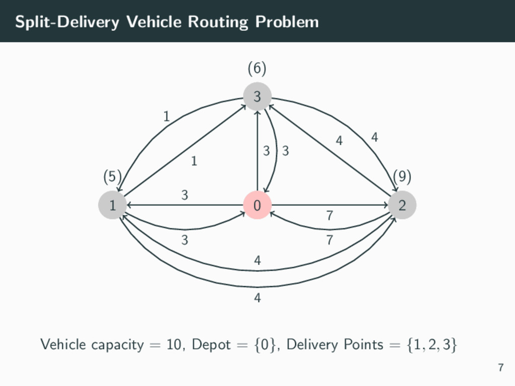
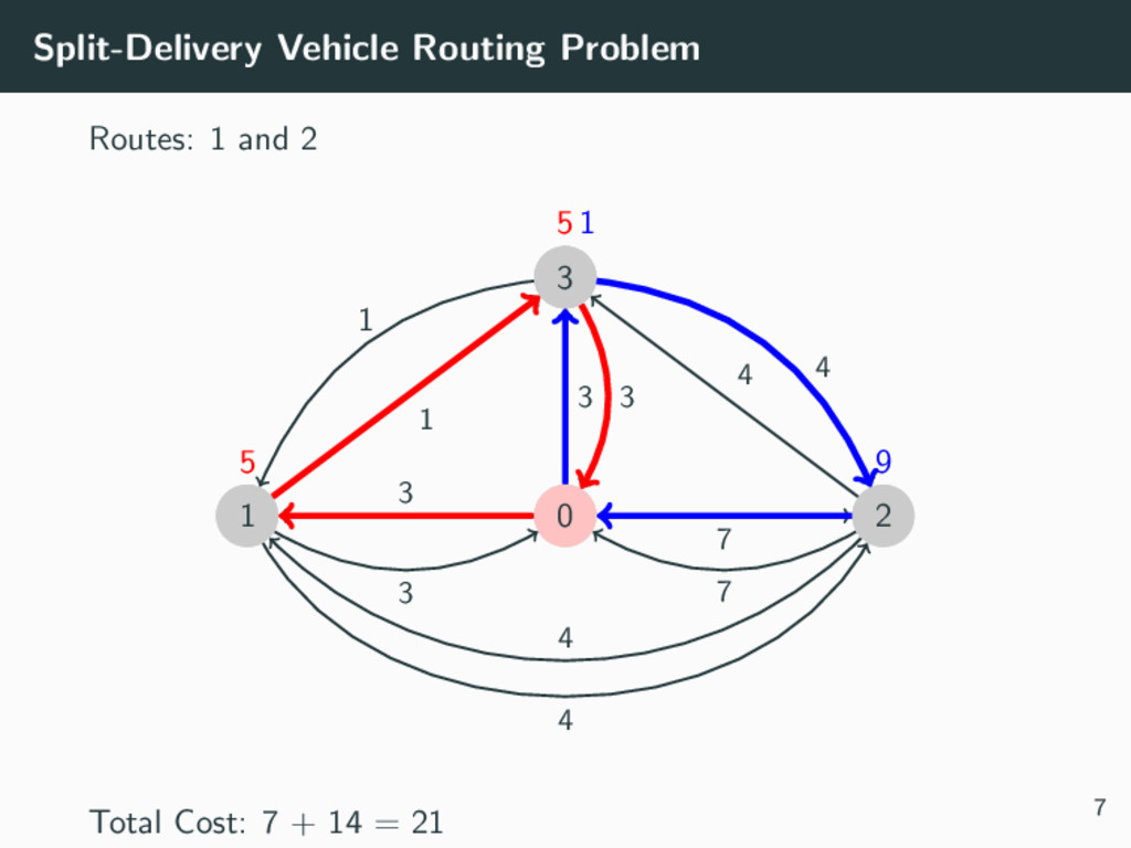
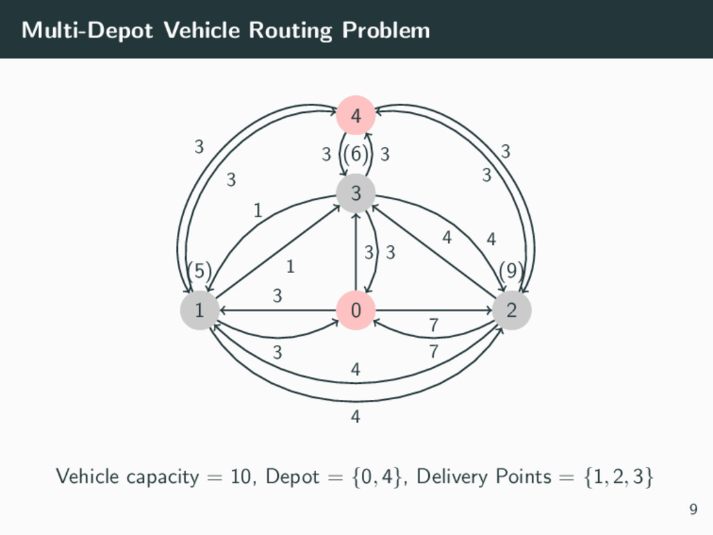
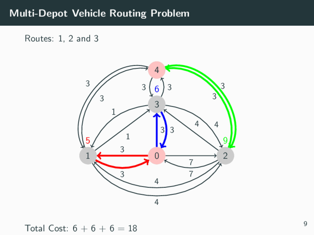
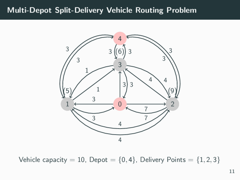
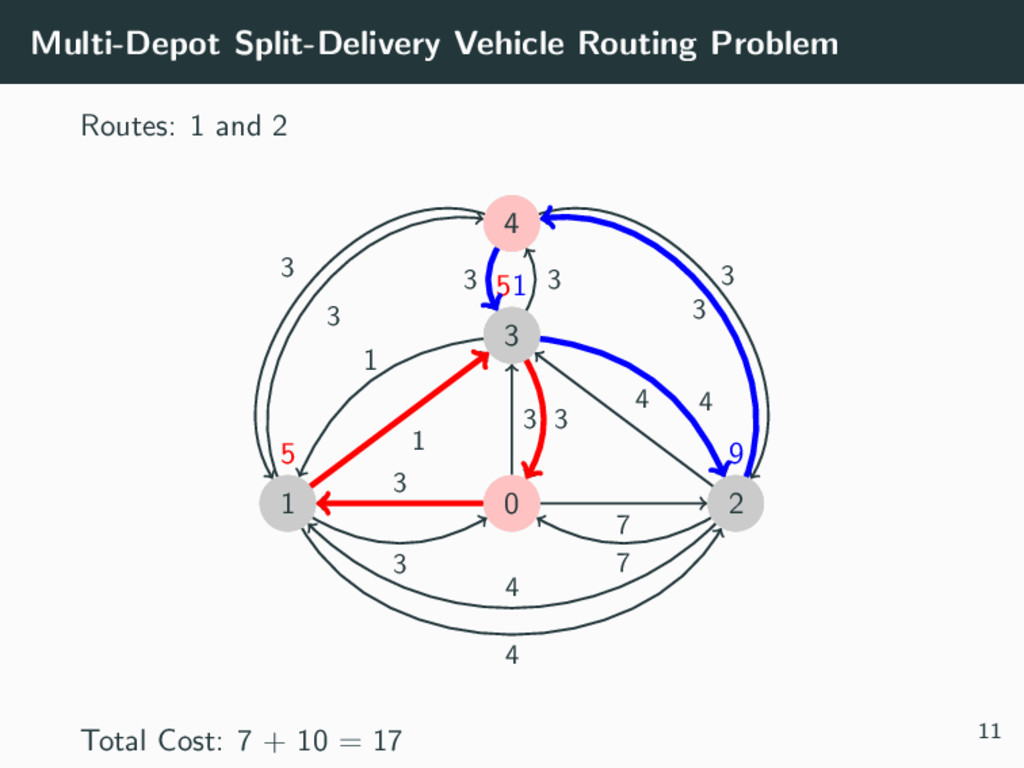
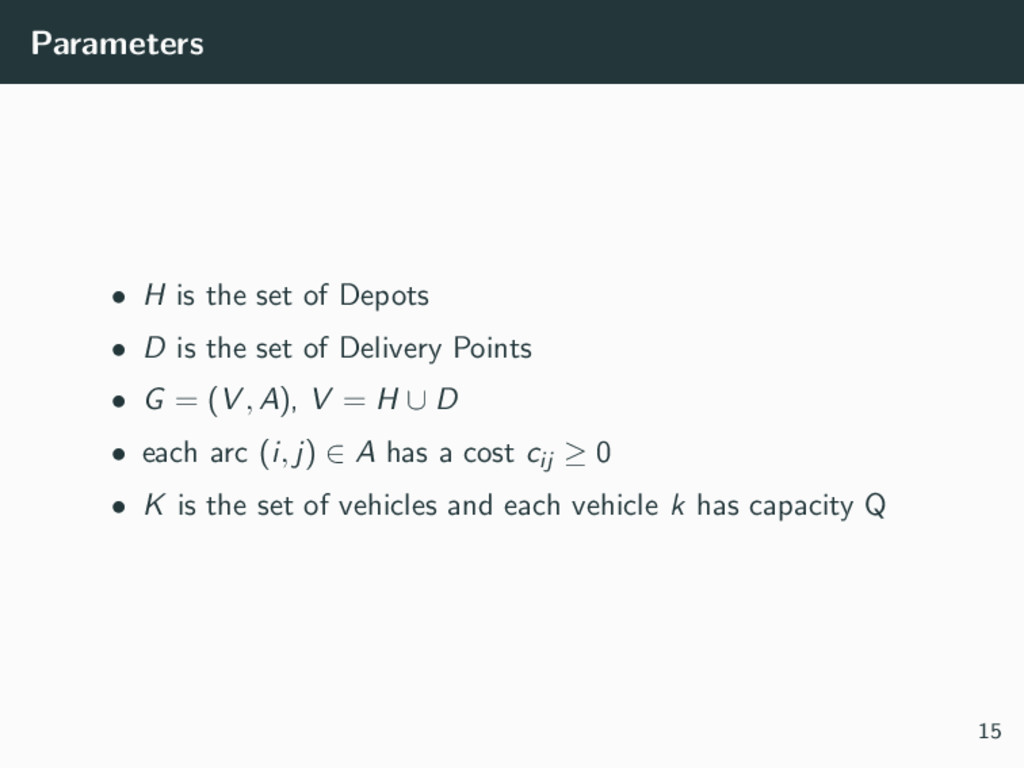
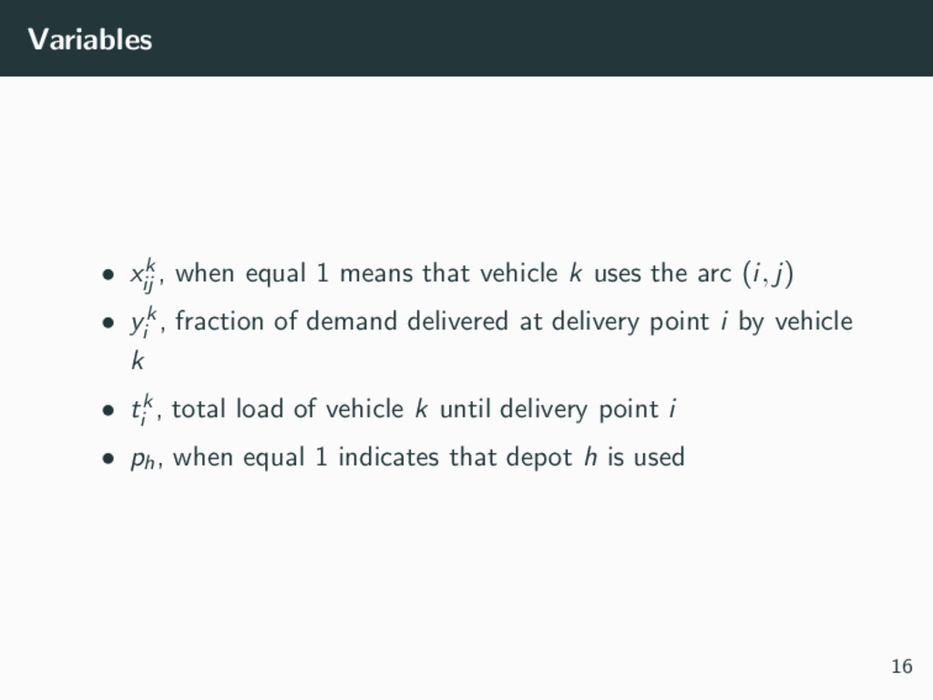
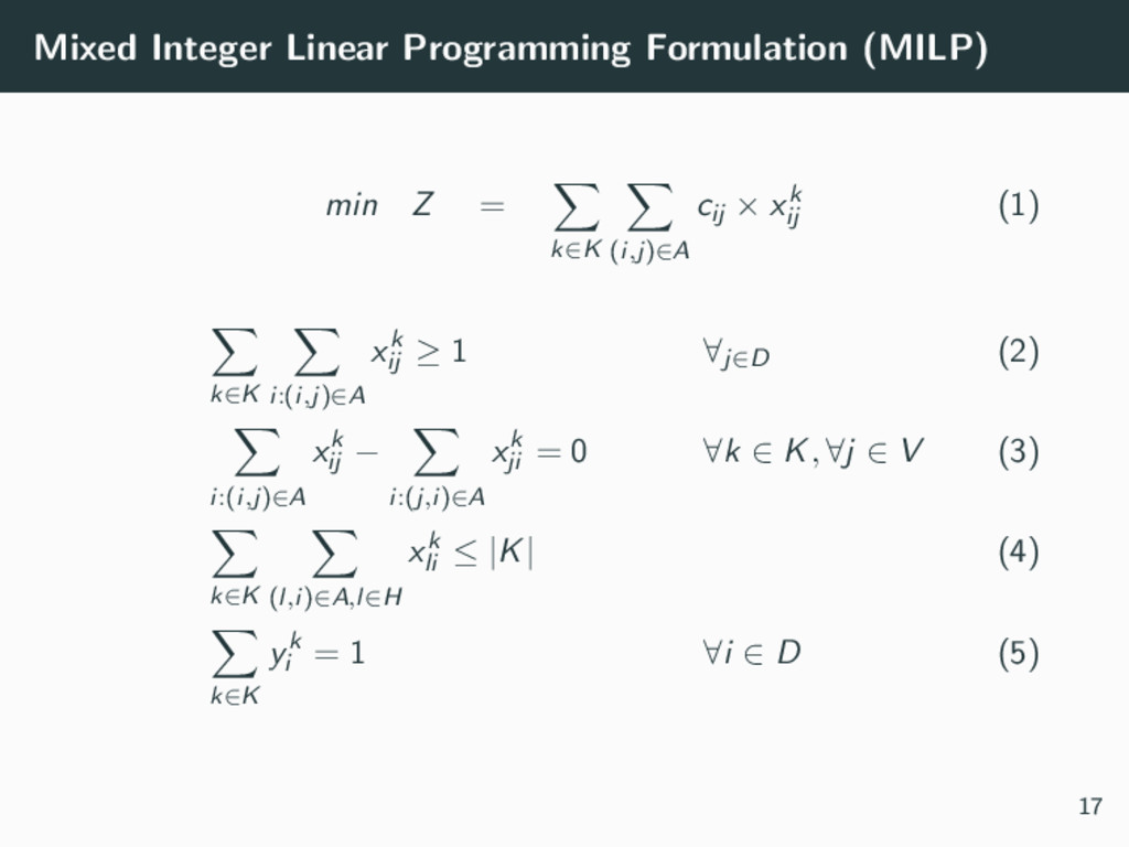
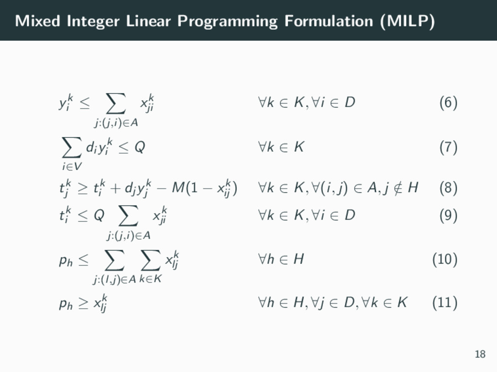
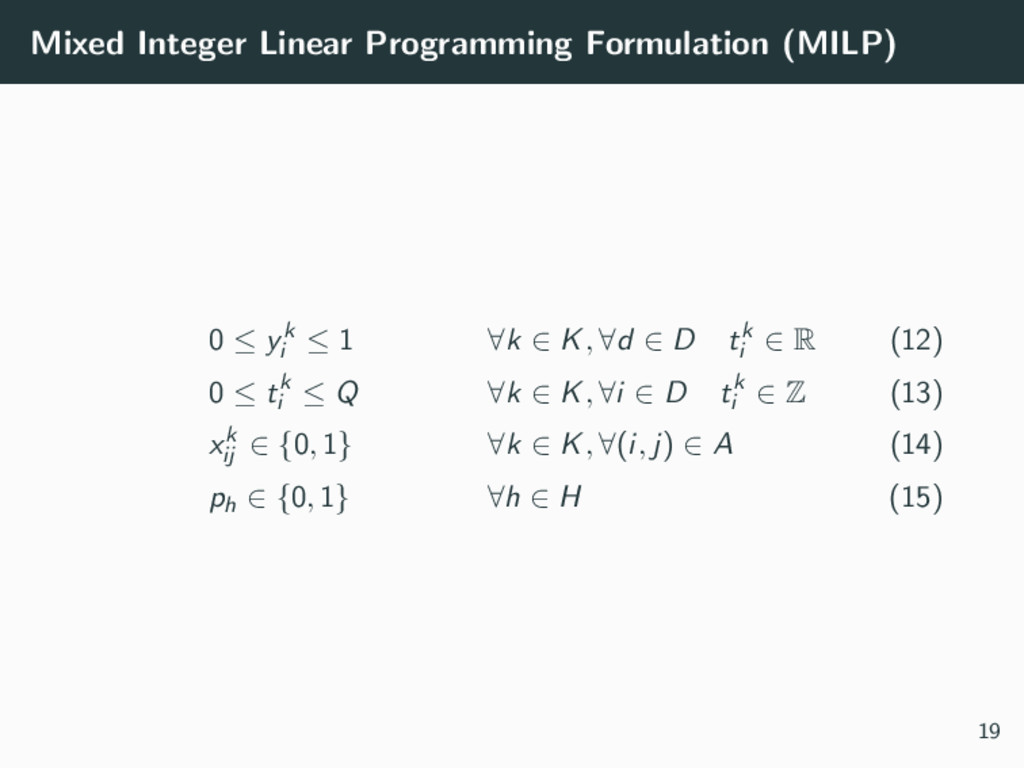
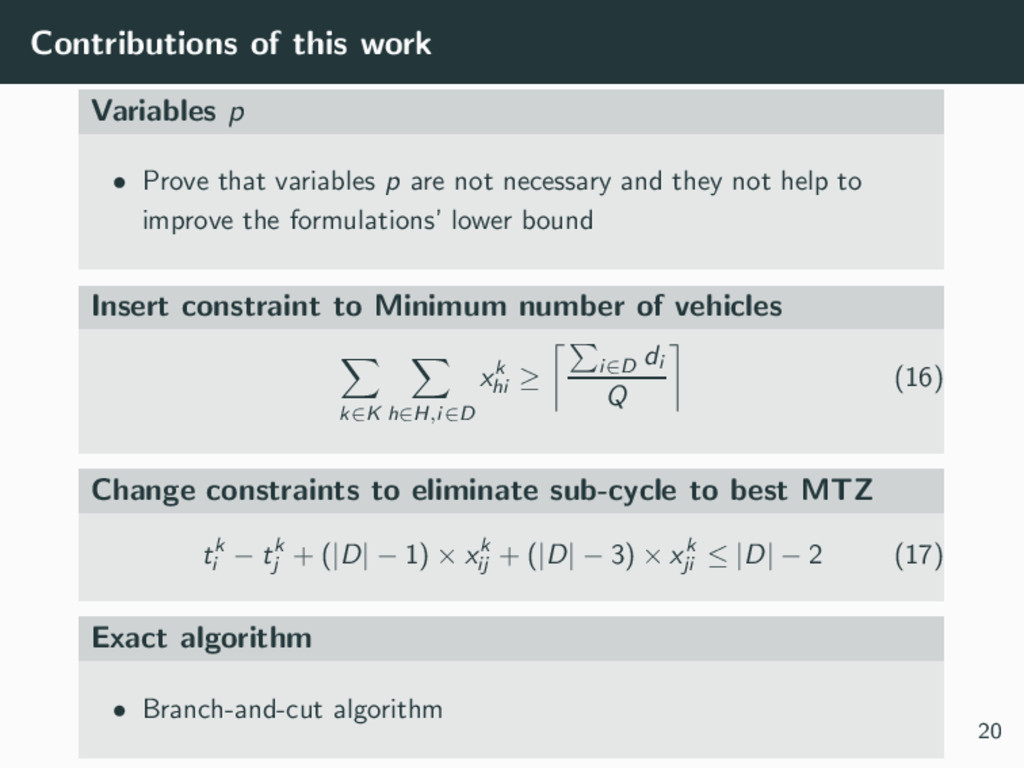
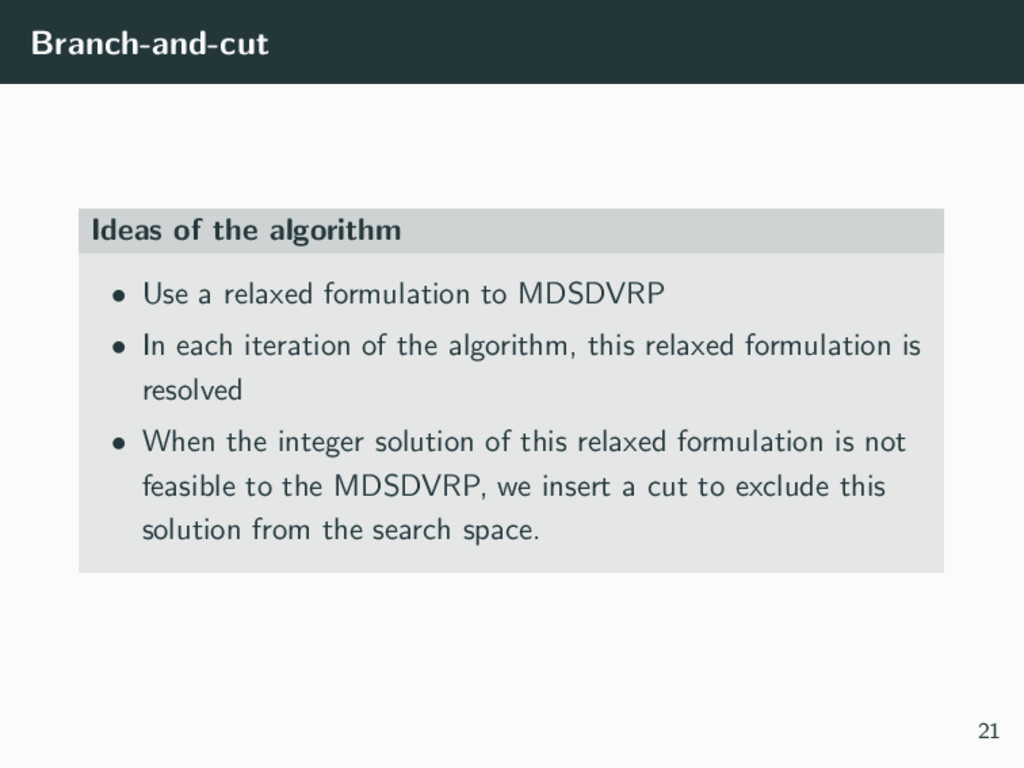
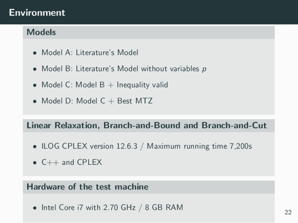
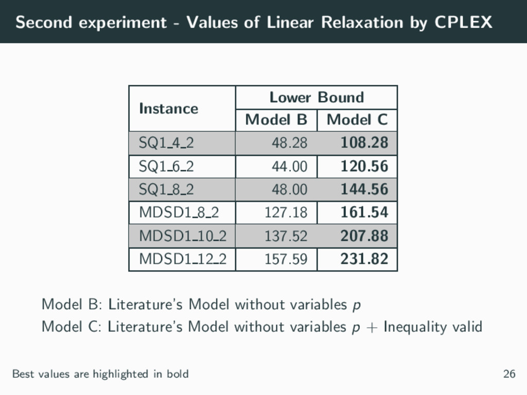
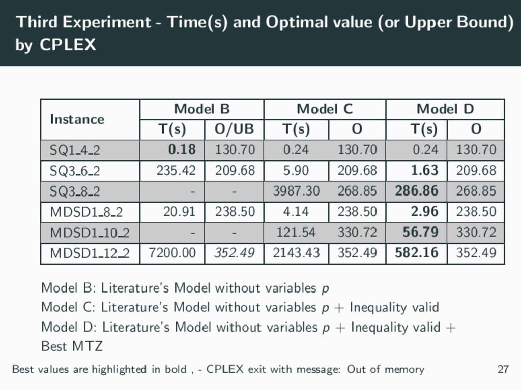
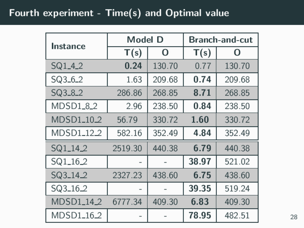
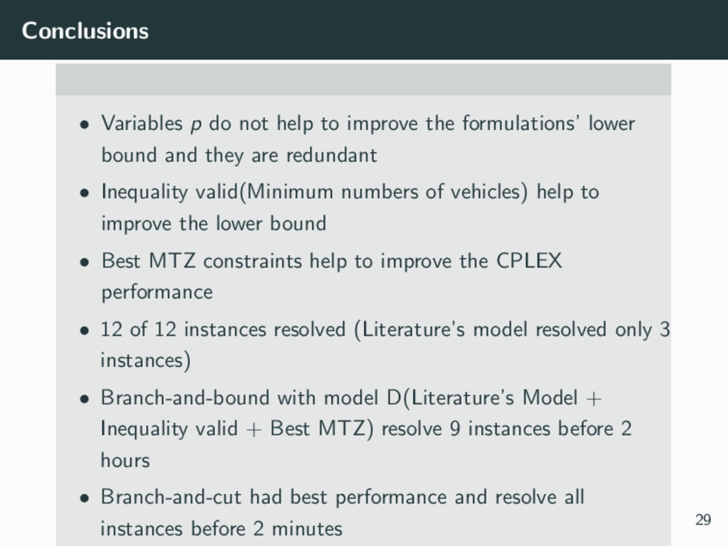
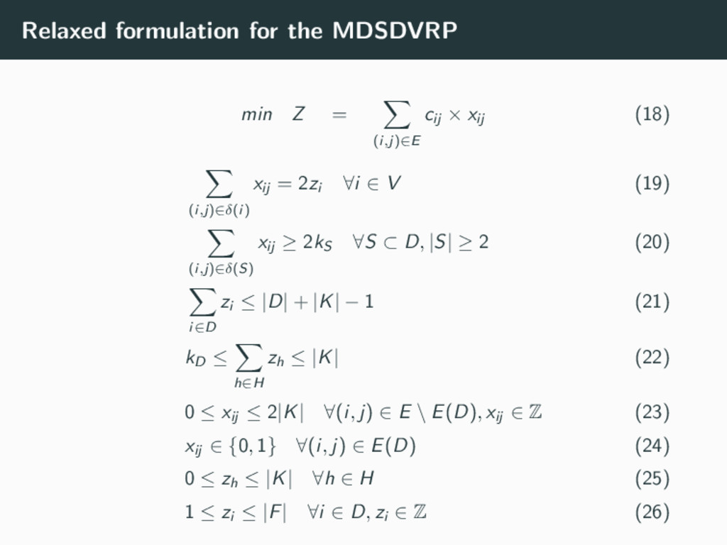
Presentation about the problem Multi-Depot Split-Delivery Vehicle Routing Problem at Université de Technologie de Troyes. In this presentation I showed that first 6 months of my work in this problem. I proposed a new branch and cut for this problem and improve the math model present in the literature.

Transcript

1. Innovative strategies to the shared transport of humanitarian aid and goods Multi-Depot Split-Delivery Vehicle Routing Problem Jo˜ ao Carlos Abreu joao carlos.abreu junior@utt.fr Advisors: Christian Prins and Andr´ ea Cynthia Santos June 2, 2017 Universit´ e de Technologie de Troyes
2. Overview Introduction Context Vehicle Routing Problems Literature Review MDSDVRP Formulation Contributions of this work Branch-and-cut Computational Experiments Conclusions Future Works 1
3. Introduction
4. Macro-Distribution in post-disaster relief Context • Disaster (earthquakes, floods, fires) • Transferring supplies (food, drugs, watter) • Big depots (airport, ports) to intermediate depots Modeled as • Multi-Depot Split-Delivery Vehicle Routing Problem • Big depots are represented by Depots • Intermediate depots are represented by Delivery Points 2
5. Vehicle Routing Problems (VRPs) Types of VRPs • Capacitated Vehicle Routing Problem (CVRP) • Split-Delivery Vehicle Routing Problem (SDVRP) • Multi-Depot Vehicle Routing Problem (MDVRP) • Multi-Depot Split-Delivery Vehicle Routing Problem (MDSDVRP) 3
6. Vehicle Routing Problems (VRPs) Capacitated Vehicle Routing Problem (CVRP) • One Depot • Without Split-Delivery 4
7. Capacitated Vehicle Routing Problem 0 1 2 3 1 (5) 2 (9) 3 (6) 3 7 1 4 3 1 3 7 3 4 4 4 0 Vehicle capacity = 10, Depot = {0}, Delivery Points = {1, 2, 3} 5
8. Capacitated Vehicle Routing Problem Routes: 1, 2 and 3 0 1 2 3 3 7 1 4 3 1 3 7 3 4 4 4 0 1 5 2 9 3 6 Total Cost: 6 + 14 + 6 = 26 5
9. Vehicle Routing Problems (VRPs) Capacitated Vehicle Routing Problem (CVRP) • One Depot • Without Split-Delivery Split-Delivery Vehicle Routing Problem (SDVRP) • One Depot • Split-Delivery 6
10. Split-Delivery Vehicle Routing Problem 0 1 2 3 1 (5) 2 (9) 3 (6) 3 7 1 4 3 1 3 7 3 4 4 4 0 Vehicle capacity = 10, Depot = {0}, Delivery Points = {1, 2, 3} 7
11. Split-Delivery Vehicle Routing Problem Routes: 1 and 2 0 1 2 3 3 7 1 4 3 1 3 7 3 4 4 4 0 1 5 3 5 3 1 2 9 Total Cost: 7 + 14 = 21 7
12. Vehicle Routing Problems (VRPs) Capacitated Vehicle Routing Problem (CVRP) • One Depot • Without Split-Delivery Split-Delivery Vehicle Routing Problem (SDVRP) • One Depot • Split-Delivery Multi-Depot Vehicle Routing Problem (MDVRP) • Multiple Depots • Without Split-Delivery 8
13. Multi-Depot Vehicle Routing Problem 0 1 2 3 4 1 (5) 2 (9) 3 (6) 3 7 1 4 3 1 3 7 3 4 4 4 3 3 3 3 3 3 0 4 Vehicle capacity = 10, Depot = {0, 4}, Delivery Points = {1, 2, 3} 9
14. Multi-Depot Vehicle Routing Problem Routes: 1, 2 and 3 0 1 2 3 4 3 7 1 4 3 1 3 7 3 4 4 4 3 3 3 3 3 3 0 4 1 5 3 6 2 9 Total Cost: 6 + 6 + 6 = 18 9
15. Vehicle Routing Problems (VRPs) Multi-Depot Split-Delivery Vehicle Routing Problem (MDSDVRP) • Compounded by MDVRP and SDVRP • Multiple Depots • Split-Delivery 10
16. Multi-Depot Split-Delivery Vehicle Routing Problem 0 1 2 3 4 1 (5) 2 (9) 3 (6) 3 7 1 4 3 1 3 7 3 4 4 4 3 3 3 3 3 3 0 4 Vehicle capacity = 10, Depot = {0, 4}, Delivery Points = {1, 2, 3} 11
17. Multi-Depot Split-Delivery Vehicle Routing Problem Routes: 1 and 2 0 1 2 3 4 3 7 1 4 3 1 3 7 3 4 4 4 3 3 3 3 3 3 0 4 1 5 3 5 2 9 3 1 Total Cost: 7 + 10 = 17 11
18. Literature Review Authors Article’s Name Year D. Gulczynski, B. Golden, E. Wasil The multi-depot split delivery vehicle routing problem: an integer programming-based heuristic, new test problems, and computational results 2011 A. Soeanu, et. al. A decentralized heuristic for multi-depot split-delivery vehicle routing problem 2011 S. Ray, et. al. Modeling multi-depot split-delivery vehicle routing problem 2012 S. Ray, et. al. The multi-depot split-delivery vehicle routing problem: Model and solution algorithm 2014 A. C. Santos Shared transportation for macro-distribution in post-disaster relief 2015 12
19. Literature Review Authors Article’s Name Year E H G. Laporte The Vehicle Routing Problem: An overview of exact and approximate algorithms 1992 * * C. Archetti, M. Speranza The split delivery vehicle routing problem: a survey 2008 * D. J. Gulczynski, B. Golden, E. Wasil Recent Developments in Modeling and Solving the Split Delivery Vehicle Routing Problem 2008 * * J. M. Belenguer, et. al. A Branch-and-cut method for the Capacitated Location-Routing Problem 2011 * T. Bektas, L. Gouveia Requiem for the Miller-Tucker-Zemlin subtour elimination constraints? 2014 E = Exact algorithms, H = Heuristics 13
20. Literature Review Authors Article’s Name Year E H I. Muter, J. F. Cordeau, G. Laporte A Branc-and-Price algorithm for the Multi-depot Vehicle Routing Problem with Interdepot Routes 2014 * C. Archetti, N. Bianchessi, M. G. Speranza Branch-and-Cut algorithms for the split delivery vehicle routing problem 2014 * J. R. Montoya-Torres, et. al. A literature review on the vehicle routing problems with multiple depots 2015 * * K. Braekers, et. al. The vehicle routing problem: State of the art classification and review 2016 * * E = Exact algorithms, H = Heuristics 14
21. MDSDVRP Formulation
22. Parameters • H is the set of Depots • D is the set of Delivery Points • G = (V , A), V = H ∪ D • each arc (i, j) ∈ A has a cost cij ≥ 0 • K is the set of vehicles and each vehicle k has capacity Q 15
23. Variables • xk ij , when equal 1 means that vehicle k uses the arc (i, j) • yk i , fraction of demand delivered at delivery point i by vehicle k • tk i , total load of vehicle k until delivery point i • ph, when equal 1 indicates that depot h is used 16
24. Mixed Integer Linear Programming Formulation (MILP) min Z = k∈K (i,j)∈A cij × xk ij (1) k∈K i:(i,j)∈A xk ij ≥ 1 ∀j∈D (2) i:(i,j)∈A xk ij − i:(j,i)∈A xk ji = 0 ∀k ∈ K, ∀j ∈ V (3) k∈K (l,i)∈A,l∈H xk li ≤ |K| (4) k∈K yk i = 1 ∀i ∈ D (5) 17
25. Mixed Integer Linear Programming Formulation (MILP) yk i ≤ j:(j,i)∈A xk ji ∀k ∈ K, ∀i ∈ D (6) i∈V di yk i ≤ Q ∀k ∈ K (7) tk j ≥ tk i + dj yk j − M(1 − xk ij ) ∀k ∈ K, ∀(i, j) ∈ A, j / ∈ H (8) tk i ≤ Q j:(j,i)∈A xk ji ∀k ∈ K, ∀i ∈ D (9) ph ≤ j:(l,j)∈A k∈K xk lj ∀h ∈ H (10) ph ≥ xk lj ∀h ∈ H, ∀j ∈ D, ∀k ∈ K (11) 18
26. Mixed Integer Linear Programming Formulation (MILP) 0 ≤ yk i ≤ 1 ∀k ∈ K, ∀d ∈ D tk i ∈ R (12) 0 ≤ tk i ≤ Q ∀k ∈ K, ∀i ∈ D tk i ∈ Z (13) xk ij ∈ {0, 1} ∀k ∈ K, ∀(i, j) ∈ A (14) ph ∈ {0, 1} ∀h ∈ H (15) 19
27. Contributions of this work
28. Contributions of this work Variables p • Prove that variables p are not necessary and they not help to improve the formulations’ lower bound Insert constraint to Minimum number of vehicles k∈K h∈H,i∈D xk hi ≥ i∈D di Q (16) Change constraints to eliminate sub-cycle to best MTZ tk i − tk j + (|D| − 1) × xk ij + (|D| − 3) × xk ji ≤ |D| − 2 (17) Exact algorithm • Branch-and-cut algorithm 20
29. Branch-and-cut Ideas of the algorithm • Use a relaxed formulation to MDSDVRP • In each iteration of the algorithm, this relaxed formulation is resolved • When the integer solution of this relaxed formulation is not feasible to the MDSDVRP, we insert a cut to exclude this solution from the search space. 21
30. Computational Experiments
31. Environment Models • Model A: Literature’s Model • Model B: Literature’s Model without variables p • Model C: Model B + Inequality valid • Model D: Model C + Best MTZ Linear Relaxation, Branch-and-Bound and Branch-and-Cut • ILOG CPLEX version 12.6.3 / Maximum running time 7,200s • C++ and CPLEX Hardware of the test machine • Intel Core i7 with 2.70 GHz / 8 GB RAM 22
32. Instances Instance # Depots # Delivery Points Vehicle Capacity Demands Min Max SQ1 4 2 2 4 100 60 90 SQ3 6 2 2 6 100 60 90 SQ3 8 2 2 8 100 55 90 MDSD1 8 2 2 8 80 20 70 MDSD1 10 2 2 10 80 20 70 MDSD1 12 2 2 12 80 13 70 SQ1 14 2 2 14 100 60 90 SQ1 16 2 2 16 100 55 90 SQ3 14 2 2 14 100 55 90 SQ3 16 2 2 16 80 55 90 MDSD1 14 2 2 14 80 13 70 MDSD1 16 2 2 16 80 13 70 23
33. Experiments First - Variables p help to improve the lower bound? • Compare values of models relaxations A and B Second - Valid Inequality help to improve the lower bound? • Compare values of models relaxations B and C Third - What is the best model? • Compare time and Optimal value (or Upper Bound) of Branch-and-bound(CPLEX) with models B, C and D Fourth - What is the performance of the Branch-and-cut algorithm? • Compare time and Optimal value of Branch-and-Cut with results of the best Branch-and-bound from second experiment 24
34. First experiment - Values of Linear Relaxation by CPLEX Instance Lower Bound Model A Model B SQ1 4 2 48.28 48.28 SQ1 6 2 44.00 44.00 SQ1 8 2 48.00 48.00 MDSD1 8 2 127.18 127.18 MDSD1 10 2 137.52 137.52 MDSD1 12 2 157.59 157.59 Model A: Literature’s Model Model B: Literature’s Model without variables p Best values are highlighted in bold 25
35. Second experiment - Values of Linear Relaxation by CPLEX Instance Lower Bound Model B Model C SQ1 4 2 48.28 108.28 SQ1 6 2 44.00 120.56 SQ1 8 2 48.00 144.56 MDSD1 8 2 127.18 161.54 MDSD1 10 2 137.52 207.88 MDSD1 12 2 157.59 231.82 Model B: Literature’s Model without variables p Model C: Literature’s Model without variables p + Inequality valid Best values are highlighted in bold 26
36. Third Experiment - Time(s) and Optimal value (or Upper Bound) by CPLEX Instance Model B Model C Model D T(s) O/UB T(s) O T(s) O SQ1 4 2 0.18 130.70 0.24 130.70 0.24 130.70 SQ3 6 2 235.42 209.68 5.90 209.68 1.63 209.68 SQ3 8 2 - - 3987.30 268.85 286.86 268.85 MDSD1 8 2 20.91 238.50 4.14 238.50 2.96 238.50 MDSD1 10 2 - - 121.54 330.72 56.79 330.72 MDSD1 12 2 7200.00 352.49 2143.43 352.49 582.16 352.49 Model B: Literature’s Model without variables p Model C: Literature’s Model without variables p + Inequality valid Model D: Literature’s Model without variables p + Inequality valid + Best MTZ Best values are highlighted in bold , - CPLEX exit with message: Out of memory 27
37. Fourth experiment - Time(s) and Optimal value Instance Model D Branch-and-cut T(s) O T(s) O SQ1 4 2 0.24 130.70 0.77 130.70 SQ3 6 2 1.63 209.68 0.74 209.68 SQ3 8 2 286.86 268.85 8.71 268.85 MDSD1 8 2 2.96 238.50 0.84 238.50 MDSD1 10 2 56.79 330.72 1.60 330.72 MDSD1 12 2 582.16 352.49 4.84 352.49 SQ1 14 2 2519.30 440.38 6.79 440.38 SQ1 16 2 - - 38.97 521.02 SQ3 14 2 2327.23 438.60 6.75 438.60 SQ3 16 2 - - 39.35 519.24 MDSD1 14 2 6777.34 409.30 6.83 409.30 MDSD1 16 2 - - 78.95 482.51 28
38. Conclusions
39. Conclusions • Variables p do not help to improve the formulations’ lower bound and they are redundant • Inequality valid(Minimum numbers of vehicles) help to improve the lower bound • Best MTZ constraints help to improve the CPLEX performance • 12 of 12 instances resolved (Literature’s model resolved only 3 instances) • Branch-and-bound with model D(Literature’s Model + Inequality valid + Best MTZ) resolve 9 instances before 2 hours • Branch-and-cut had best performance and resolve all instances before 2 minutes 29
40. Future Works
41. Future Works Literature Review • SDVRP and MDVRP • Best cuts to improve lower bound in VRP Exact Algorithms • Adapt the model MDVRP to MDSDVRP • Local branching • Branch-and-price Heuristics • Adapt the best heuristics from SDVRP to MDSDVRP • Adapt the best heuristics from MDVRP to MDSDVRP • Large Scale 30
42. Thank you! 30
43. Relaxed Formulation
44. Parameters • H is the set of Depots • D is the set of Delivery Points • G = (V , E), V = H ∪ D, E = {(i, j) : i < j; i, j ∈ V } • each arc(i, j) ∈ E has a cost cij ≥ 0 • K is the set of vehicles and each vehicle k has capacity Q • kS = i∈S di Q , minimum number of vehicles needed to serve all delivery points in set S ⊆ D • E(D) = {(i, j) ∈ E|i ∈ D, j ∈ D}, set of edges linking all pairs of delivery points • δ(S) = {(i, j)|(i ∈ S, j / ∈ S) or (i / ∈ S, j ∈ S)}, set of edges linking a node in set S with a node in V \ S
45. Variables • zi , number of visits to node i ∈ V • xij , number of times that edge (i, j) ∈ E is used
46. Relaxed formulation for the MDSDVRP min Z = (i,j)∈E cij × xij (18) (i,j)∈δ(i) xij = 2zi ∀i ∈ V (19) (i,j)∈δ(S) xij ≥ 2kS ∀S ⊂ D, |S| ≥ 2 (20) i∈D zi ≤ |D| + |K| − 1 (21) kD ≤ h∈H zh ≤ |K| (22) 0 ≤ xij ≤ 2|K| ∀(i, j) ∈ E \ E(D), xij ∈ Z (23) xij ∈ {0, 1} ∀(i, j) ∈ E(D) (24) 0 ≤ zh ≤ |K| ∀h ∈ H (25) 1 ≤ zi ≤ |F| ∀i ∈ D, zi ∈ Z (26)
47. Valid Inequalities
48. Valid Inequalities (i,j)∈δ(S) xij ≥ 2Zi ∀S ⊆ D, |S| ≥ 2, i ∈ S (27)