to enforce sparsity arg min β∈Rp 1 2 y − Xβ 2 2 data fitting + λ β 0 regularization where β 0 = card({j ∈ 1, p , βj = 0}) = card(supp(β)) Combinatorial problem; “NP-hard” Natarajan (1995) → Exact resolution requires Least-Squares (LS) solutions for all sub-models, i.e., compute LS for all possible supports (up to 2p) p = 10 → possible: ≈ 103 least squares p = 30 → hard: ≈ 1010 least squares Rem: for “small” problems mixed integer programming (MIP) well suited Bertsimas et al. (2015)
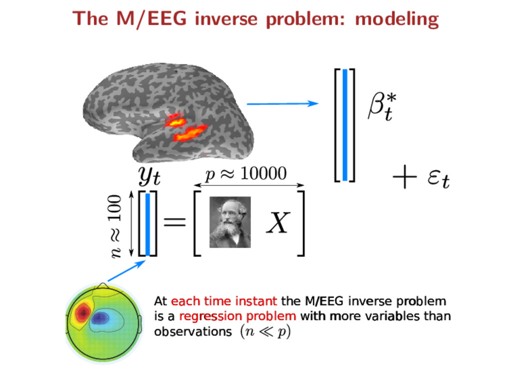
M/EEG inverse problem is a regression problem with more variables than observations At each time instant the M/EEG inverse problem is a regression problem with more variables than observations
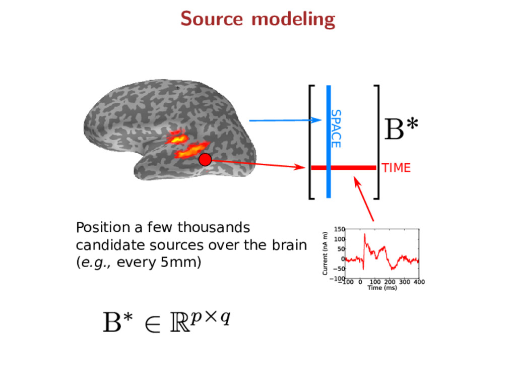
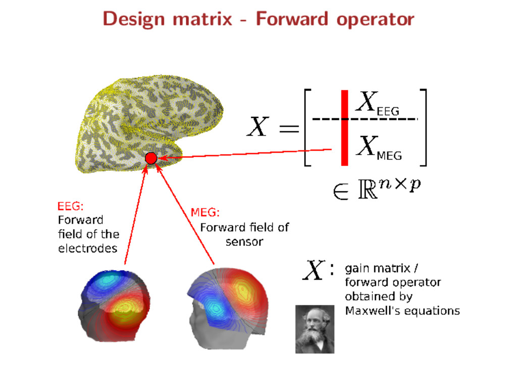
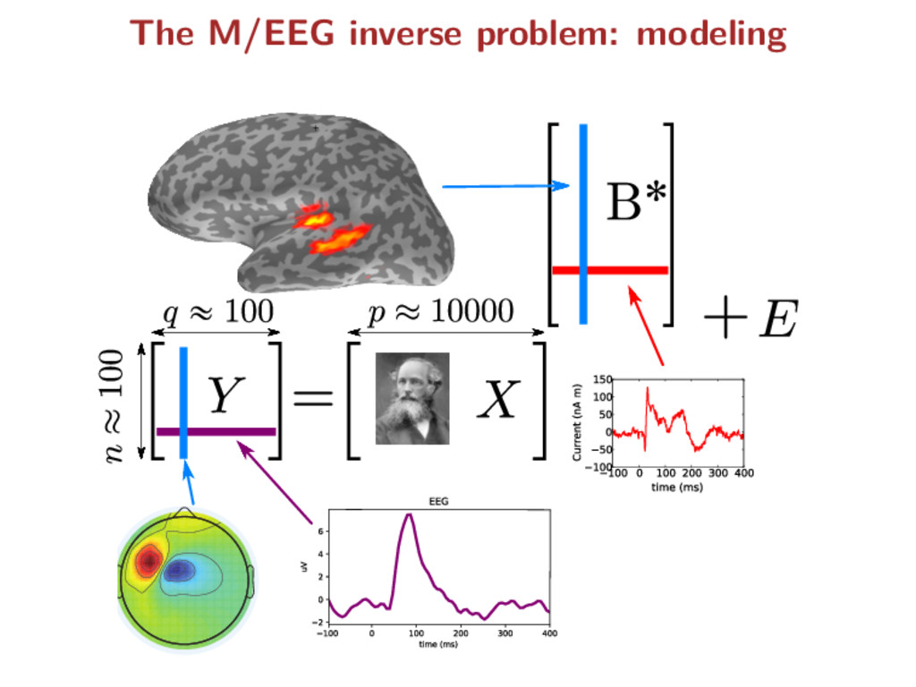
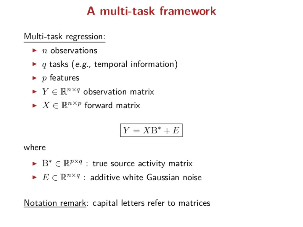
temporal information) p features Y ∈ Rn×q observation matrix X ∈ Rn×p forward matrix Y = XB∗ + E where B∗ ∈ Rp×q : true source activity matrix E ∈ Rn×q : additive white Gaussian noise Notation remark: capital letters refer to matrices
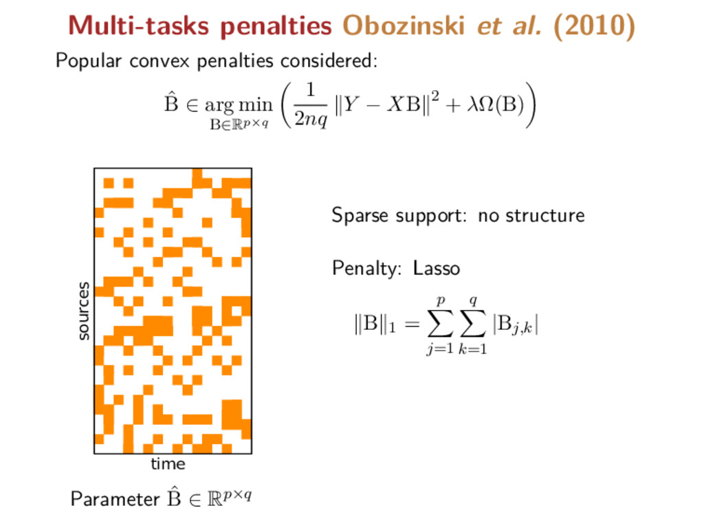
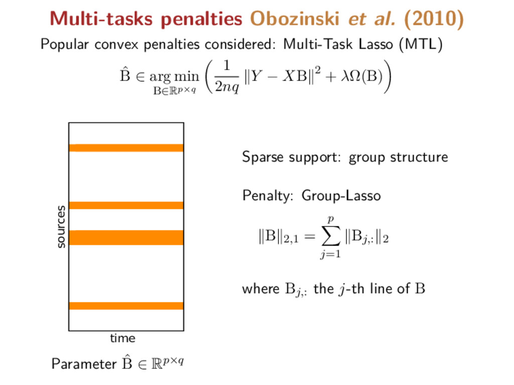
Multi-Task Lasso (MTL) ˆ B ∈ arg min B∈Rp×q 1 2nq Y − XB 2 + λΩ(B) time sources Parameter ˆ B ∈ Rp×q Sparse support: group structure Penalty: Group-Lasso B 2,1 = p j=1 Bj,: 2 where Bj,: the j-th line of B
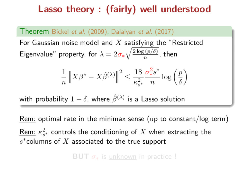
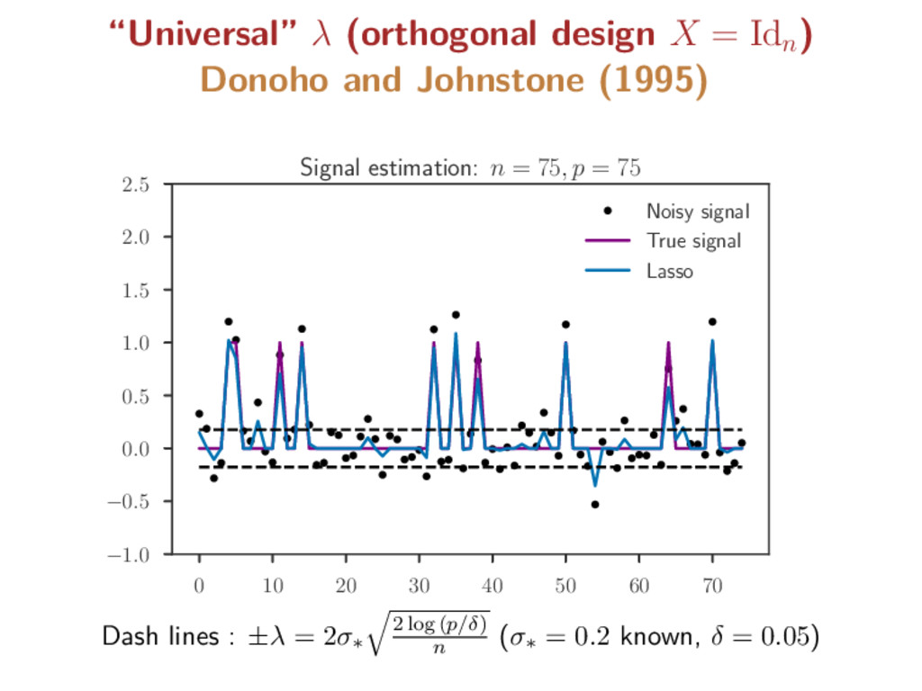
(2009), Dalalyan et al. (2017) For Gaussian noise model and X satisfying the “Restricted Eigenvalue” property, for λ = 2σ∗ 2 log (p/δ) n , then 1 n Xβ∗ − X ˆ β(λ) 2 ≤ 18 κ2 s∗ σ2 ∗ s∗ n log p δ with probability 1 − δ, where ˆ β(λ) is a Lasso solution Rem: optimal rate in the minimax sense (up to constant/log term) Rem: κ2 s∗ controls the conditioning of X when extracting the s∗columns of X associated to the true support BUT σ∗ is unknown in practice !
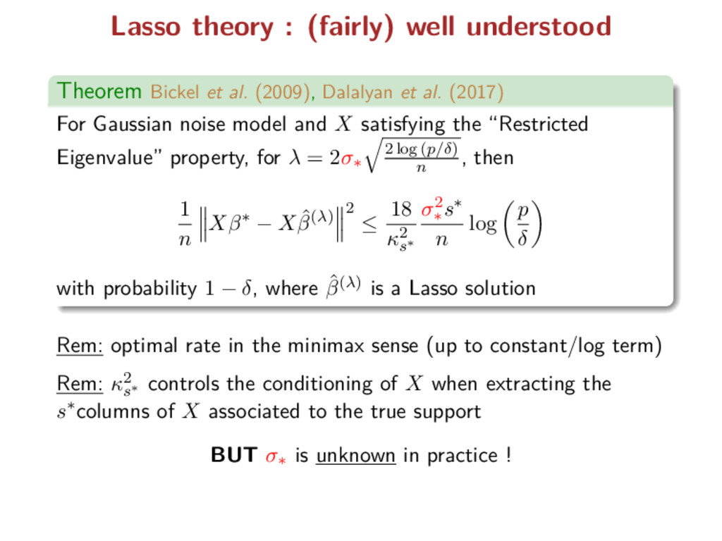
(2009), Dalalyan et al. (2017) For Gaussian noise model and X satisfying the “Restricted Eigenvalue” property, for λ = 2σ∗ 2 log (p/δ) n , then 1 n Xβ∗ − X ˆ β(λ) 2 ≤ 18 κ2 s∗ σ2 ∗ s∗ n log p δ with probability 1 − δ, where ˆ β(λ) is a Lasso solution Rem: optimal rate in the minimax sense (up to constant/log term) Rem: κ2 s∗ controls the conditioning of X when extracting the s∗columns of X associated to the true support BUT σ∗ is unknown in practice !
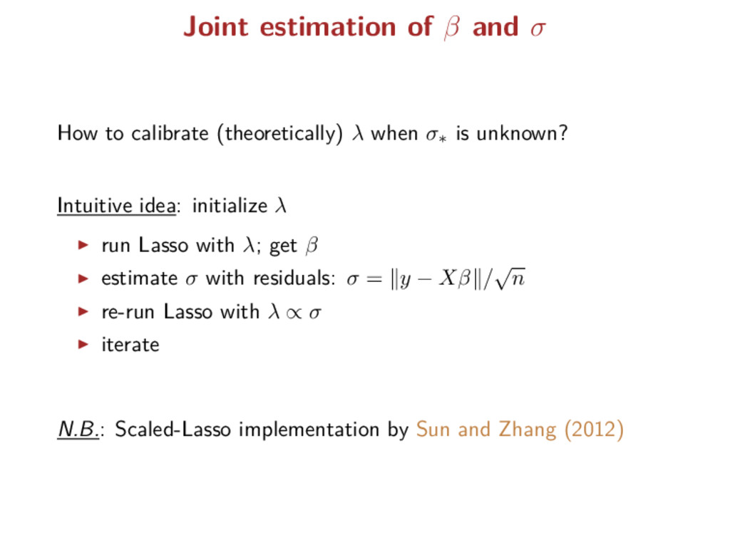
λ when σ∗ is unknown? Intuitive idea: initialize λ run Lasso with λ; get β estimate σ with residuals: σ = y − Xβ / √ n re-run Lasso with λ ∝ σ iterate N.B.: Scaled-Lasso implementation by Sun and Zhang (2012)
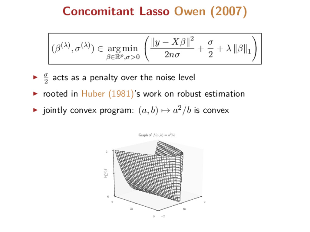
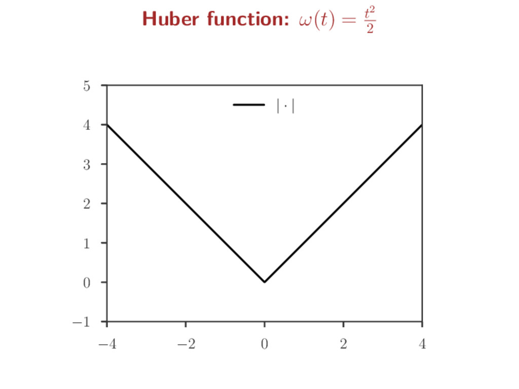
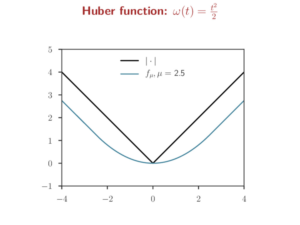
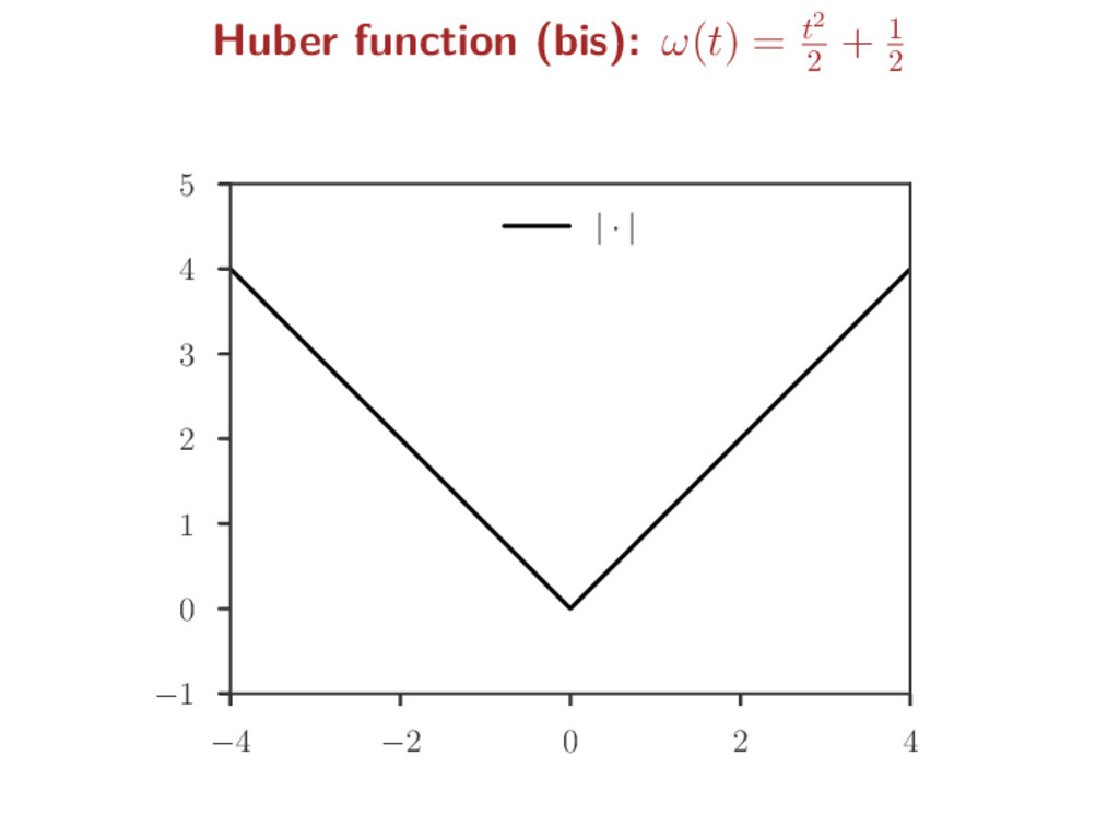
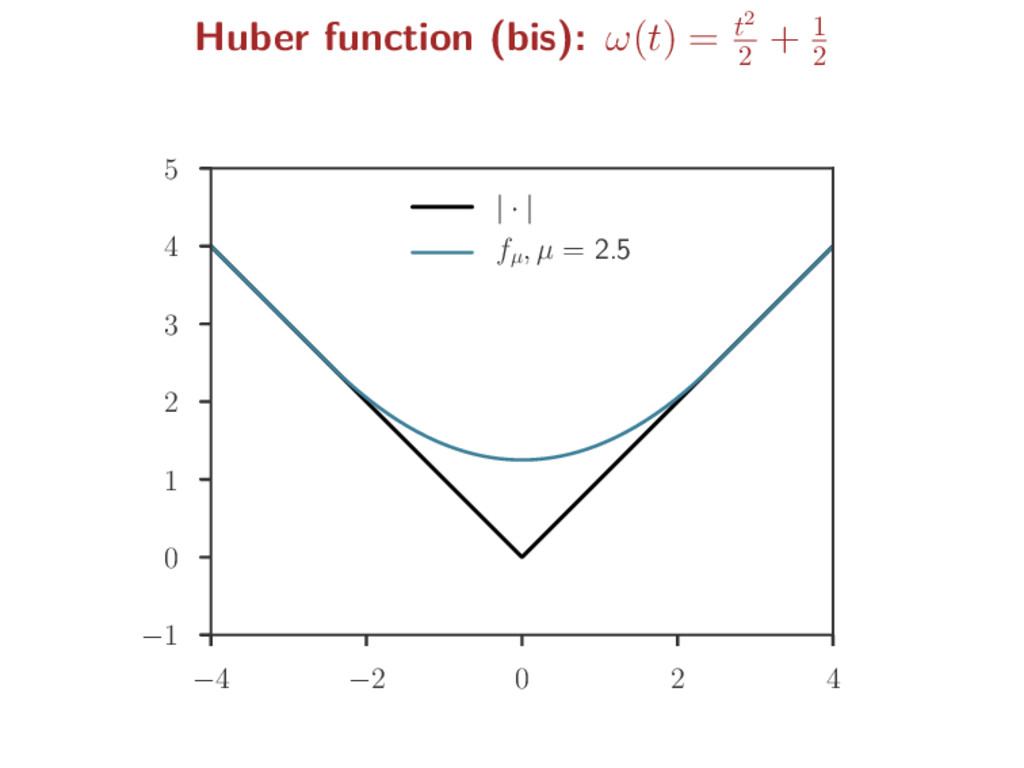
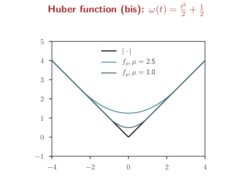
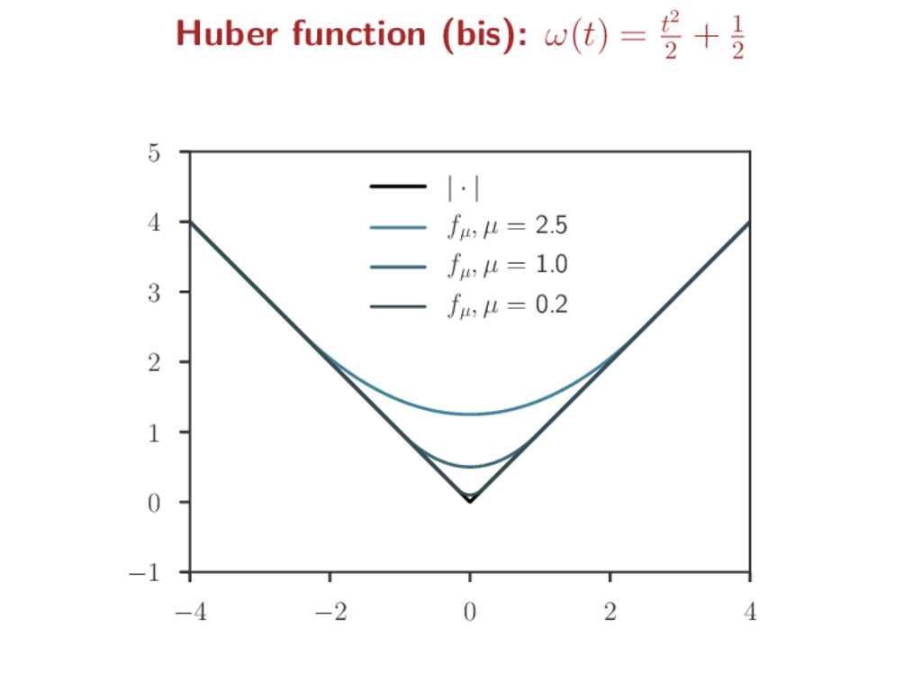
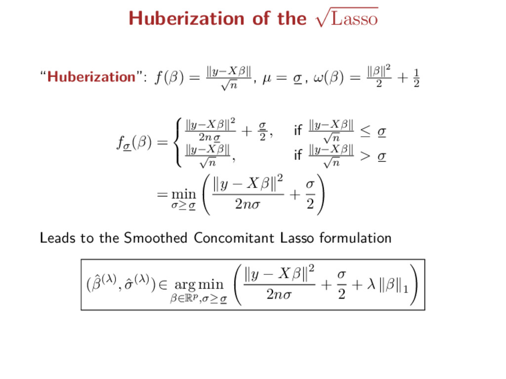
y − Xβ 2 2nσ + σ 2 + λ β 1 σ 2 acts as a penalty over the noise level rooted in Huber (1981)’s work on robust estimation jointly convex program: (a, b) → a2/b is convex a −2 0 2 b 0 1 2 f(a, b) 0 1 2 Graph of f(a, b) = a2/b
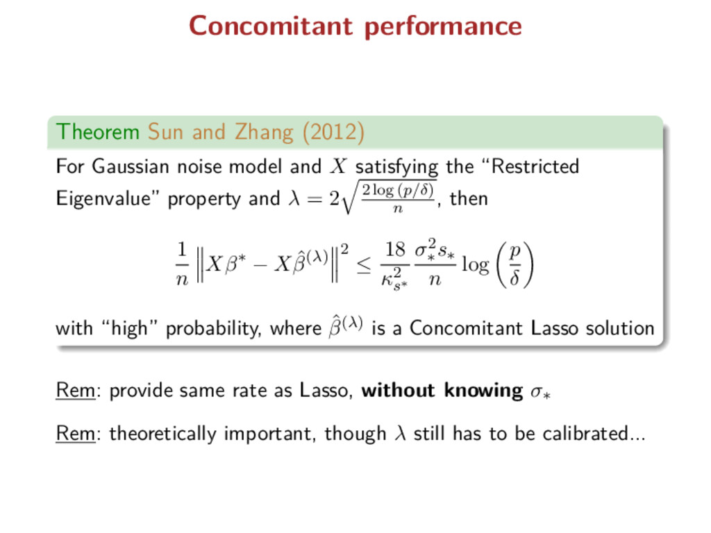
model and X satisfying the “Restricted Eigenvalue” property and λ = 2 2 log (p/δ) n , then 1 n Xβ∗ − X ˆ β(λ) 2 ≤ 18 κ2 s∗ σ2 ∗ s∗ n log p δ with “high” probability, where ˆ β(λ) is a Concomitant Lasso solution Rem: provide same rate as Lasso, without knowing σ∗ Rem: theoretically important, though λ still has to be calibrated...
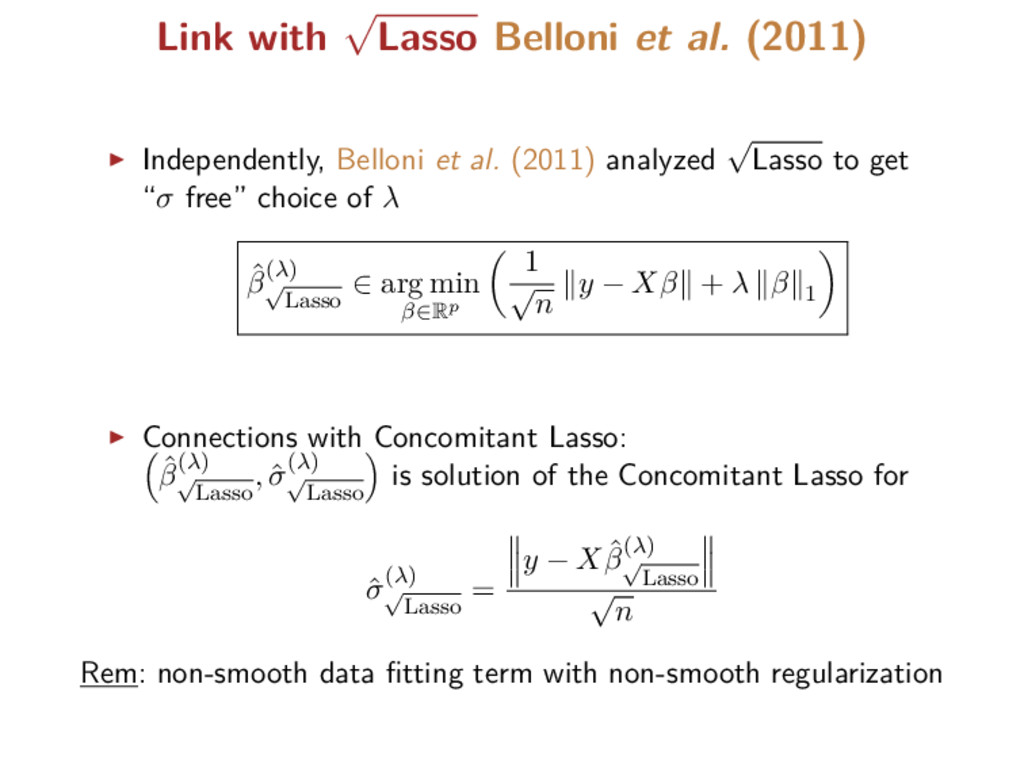
et al. (2011) analyzed √ Lasso to get “σ free” choice of λ ˆ β(λ) √ Lasso ∈ arg min β∈Rp 1 √ n y − Xβ + λ β 1 Connections with Concomitant Lasso: ˆ β(λ) √ Lasso , ˆ σ(λ) √ Lasso is solution of the Concomitant Lasso for ˆ σ(λ) √ Lasso = y − X ˆ β(λ) √ Lasso √ n Rem: non-smooth data fitting term with non-smooth regularization
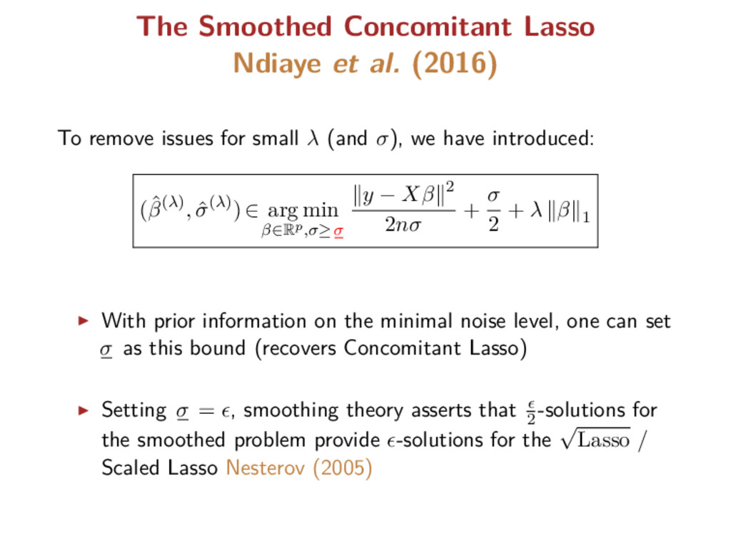
issues for small λ (and σ), we have introduced: (ˆ β(λ), ˆ σ(λ))∈ arg min β∈Rp,σ≥σ y − Xβ 2 2nσ + σ 2 + λ β 1 With prior information on the minimal noise level, one can set σ as this bound (recovers Concomitant Lasso) Setting σ = , smoothing theory asserts that 2 -solutions for the smoothed problem provide -solutions for the √ Lasso / Scaled Lasso Nesterov (2005)
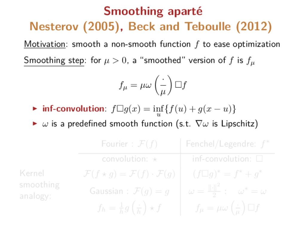
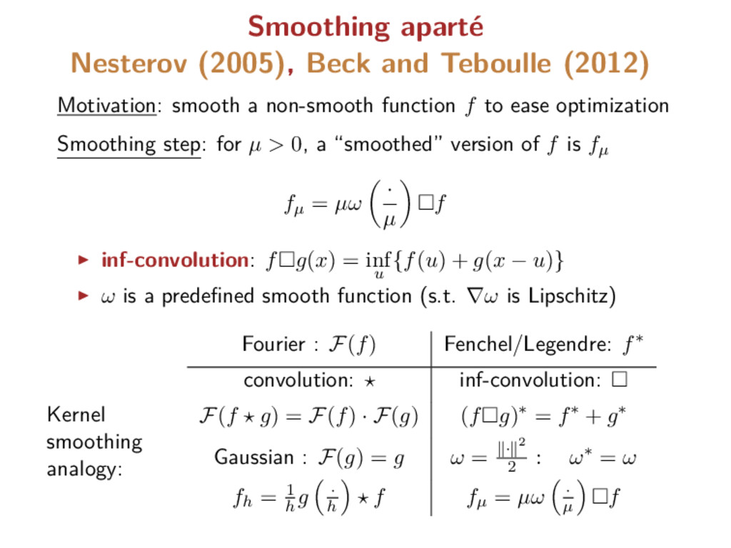
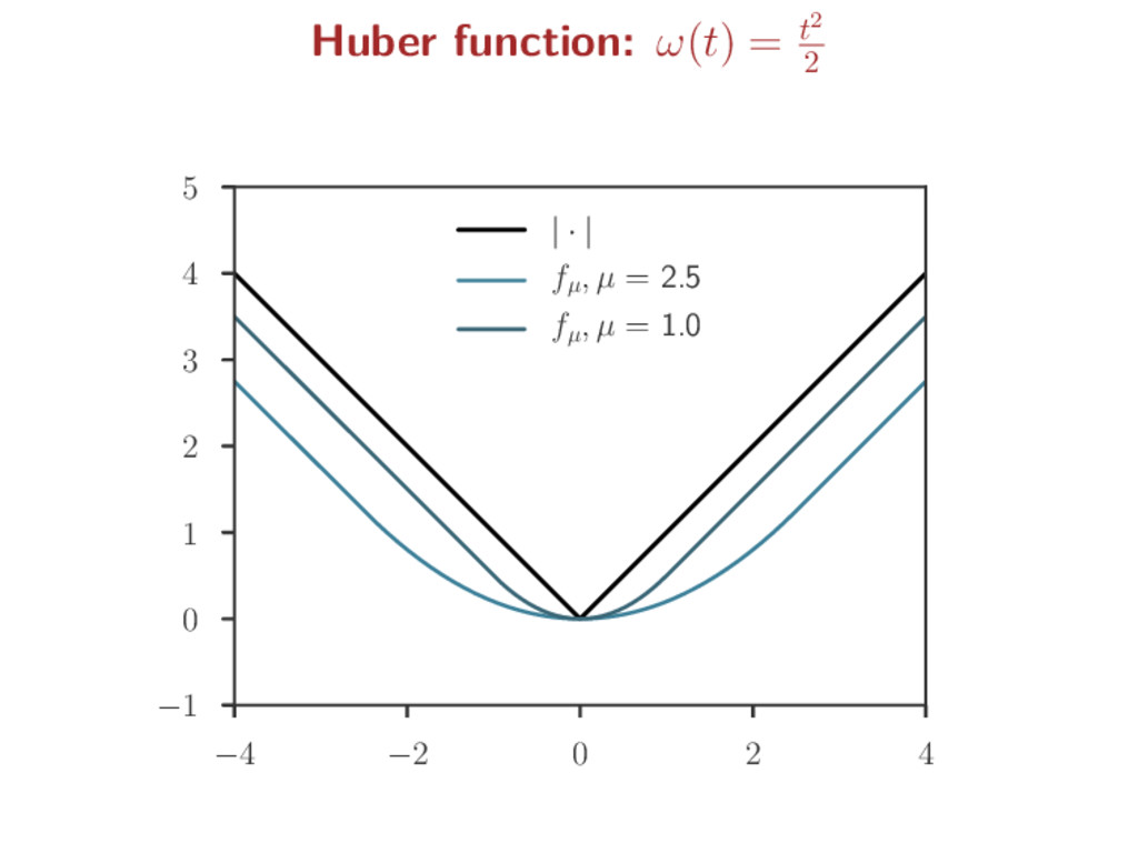
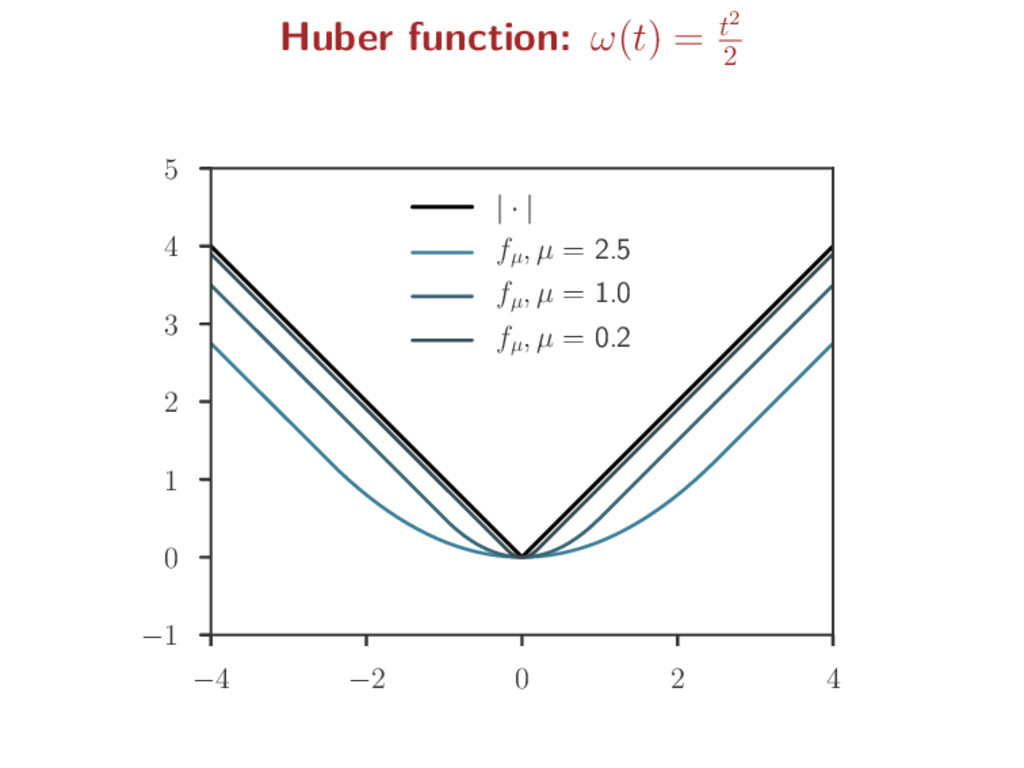
a non-smooth function f to ease optimization Smoothing step: for µ > 0, a “smoothed” version of f is fµ fµ = µω · µ f inf-convolution: f g(x) = inf u {f(u) + g(x − u)} ω is a predefined smooth function (s.t. ∇ω is Lipschitz) Kernel smoothing analogy: Fourier : F(f) Fenchel/Legendre: f∗ convolution: inf-convolution: F(f g) = F(f) · F(g) (f g)∗ = f∗ + g∗ Gaussian : F(g) = g ω = · 2 2 : ω∗ = ω fh = 1 h g · h f fµ = µω · µ f
a non-smooth function f to ease optimization Smoothing step: for µ > 0, a “smoothed” version of f is fµ fµ = µω · µ f inf-convolution: f g(x) = inf u {f(u) + g(x − u)} ω is a predefined smooth function (s.t. ∇ω is Lipschitz) Kernel smoothing analogy: Fourier : F(f) Fenchel/Legendre: f∗ convolution: inf-convolution: F(f g) = F(f) · F(g) (f g)∗ = f∗ + g∗ Gaussian : F(g) = g ω = · 2 2 : ω∗ = ω fh = 1 h g · h f fµ = µω · µ f
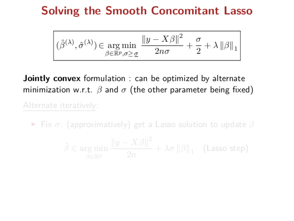
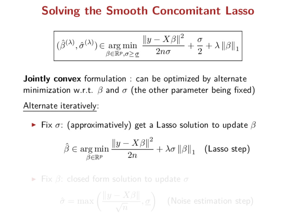
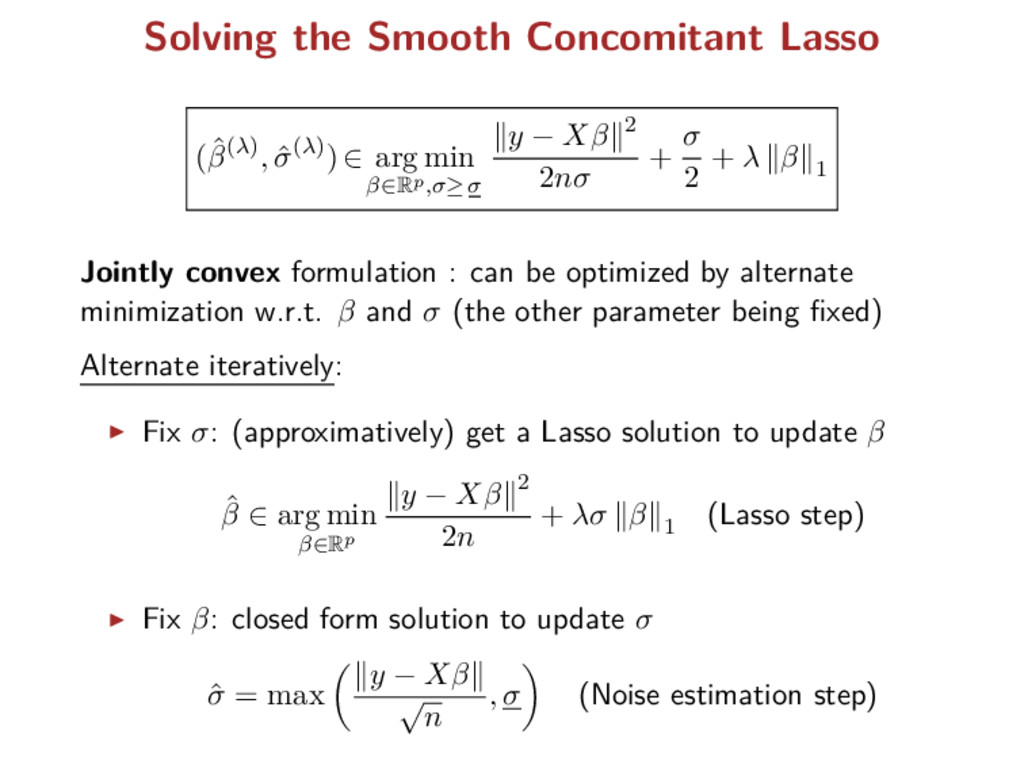
min β∈Rp,σ≥σ y − Xβ 2 2nσ + σ 2 + λ β 1 Jointly convex formulation : can be optimized by alternate minimization w.r.t. β and σ (the other parameter being fixed) Alternate iteratively: Fix σ: (approximatively) get a Lasso solution to update β ˆ β ∈ arg min β∈Rp y − Xβ 2 2n + λσ β 1 (Lasso step)
min β∈Rp,σ≥σ y − Xβ 2 2nσ + σ 2 + λ β 1 Jointly convex formulation : can be optimized by alternate minimization w.r.t. β and σ (the other parameter being fixed) Alternate iteratively: Fix σ: (approximatively) get a Lasso solution to update β ˆ β ∈ arg min β∈Rp y − Xβ 2 2n + λσ β 1 (Lasso step) Fix β: closed form solution to update σ ˆ σ = max y − Xβ √ n , σ (Noise estimation step)
min β∈Rp,σ≥σ y − Xβ 2 2nσ + σ 2 + λ β 1 Jointly convex formulation : can be optimized by alternate minimization w.r.t. β and σ (the other parameter being fixed) Alternate iteratively: Fix σ: (approximatively) get a Lasso solution to update β ˆ β ∈ arg min β∈Rp y − Xβ 2 2n + λσ β 1 (Lasso step) Fix β: closed form solution to update σ ˆ σ = max y − Xβ √ n , σ (Noise estimation step)
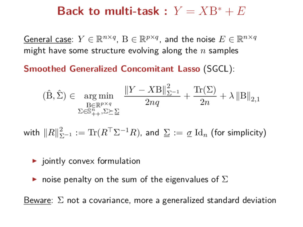
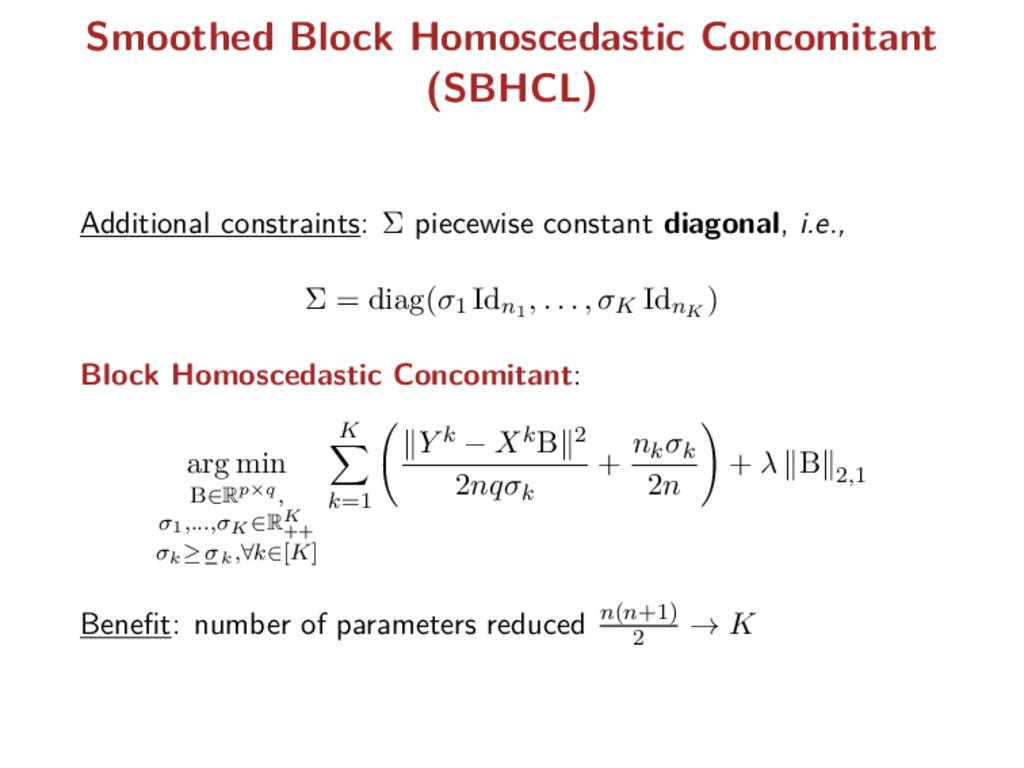
case: Y ∈ Rn×q, B ∈ Rp×q, and the noise E ∈ Rn×q might have some structure evolving along the n samples Smoothed Generalized Concomitant Lasso (SGCL): (ˆ B, ˆ Σ) ∈ arg min B∈Rp×q Σ∈Sn ++ ,Σ Σ Y − XB 2 Σ−1 2nq + Tr(Σ) 2n + λ B 2,1 with R 2 Σ−1 := Tr(R Σ−1R), and Σ := σ Idn (for simplicity) jointly convex formulation noise penalty on the sum of the eigenvalues of Σ Beware: Σ not a covariance, more a generalized standard deviation
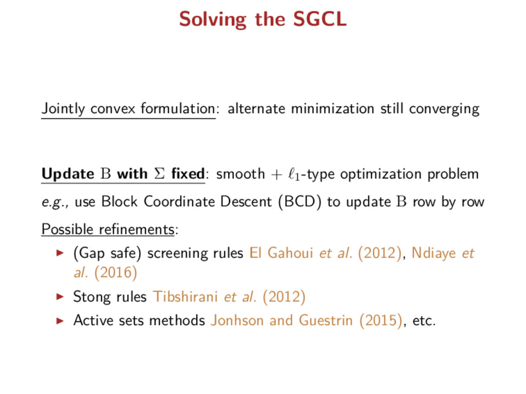
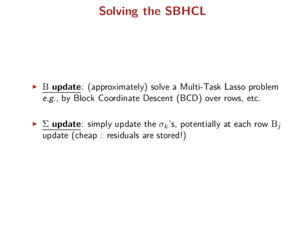
Update B with Σ fixed: smooth + 1-type optimization problem e.g., use Block Coordinate Descent (BCD) to update B row by row Possible refinements: (Gap safe) screening rules El Gahoui et al. (2012), Ndiaye et al. (2016) Stong rules Tibshirani et al. (2012) Active sets methods Jonhson and Guestrin (2015), etc.
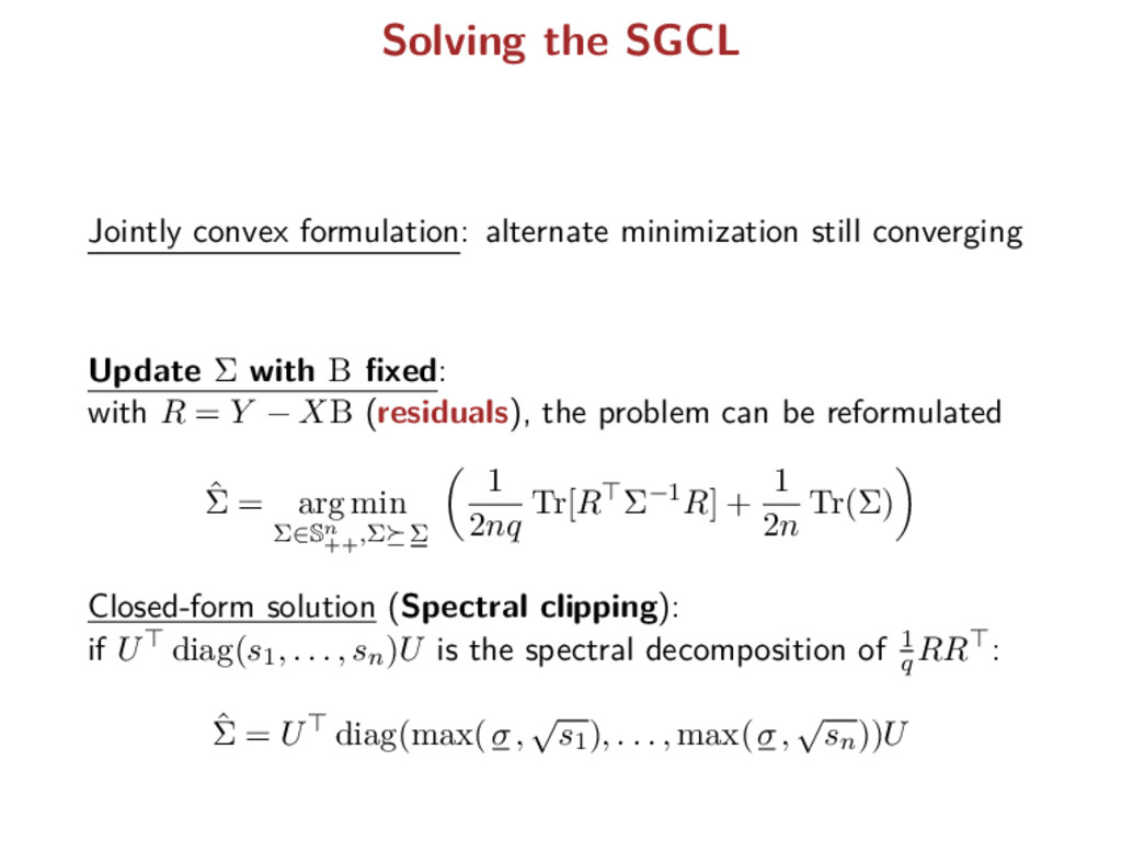
Update Σ with B fixed: with R = Y − XB (residuals), the problem can be reformulated ˆ Σ = arg min Σ∈Sn ++ ,Σ Σ 1 2nq Tr[R Σ−1R] + 1 2n Tr(Σ) Closed-form solution (Spectral clipping): if U diag(s1, . . . , sn)U is the spectral decomposition of 1 q RR : ˆ Σ = U diag(max(σ, √ s1), . . . , max(σ, √ sn))U
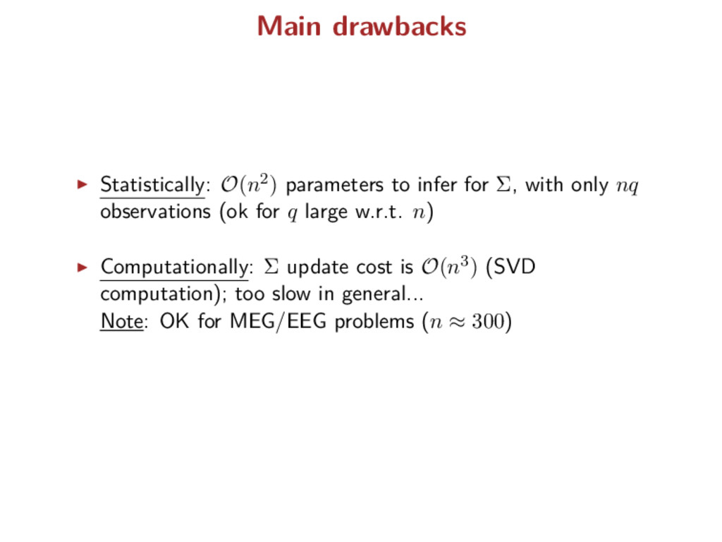
only nq observations (ok for q large w.r.t. n) Computationally: Σ update cost is O(n3) (SVD computation); too slow in general... Note: OK for MEG/EEG problems (n ≈ 300)
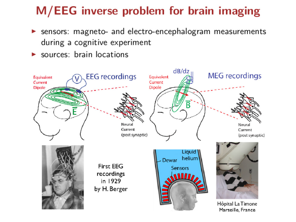
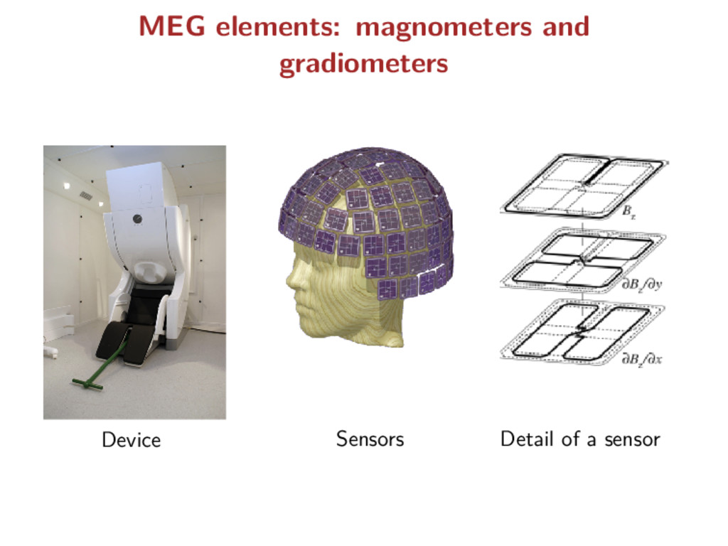
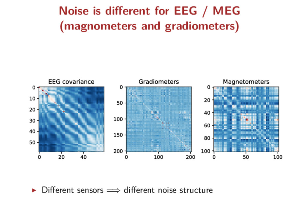
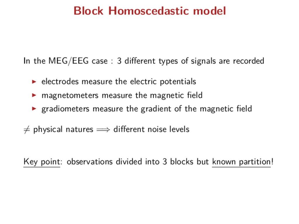
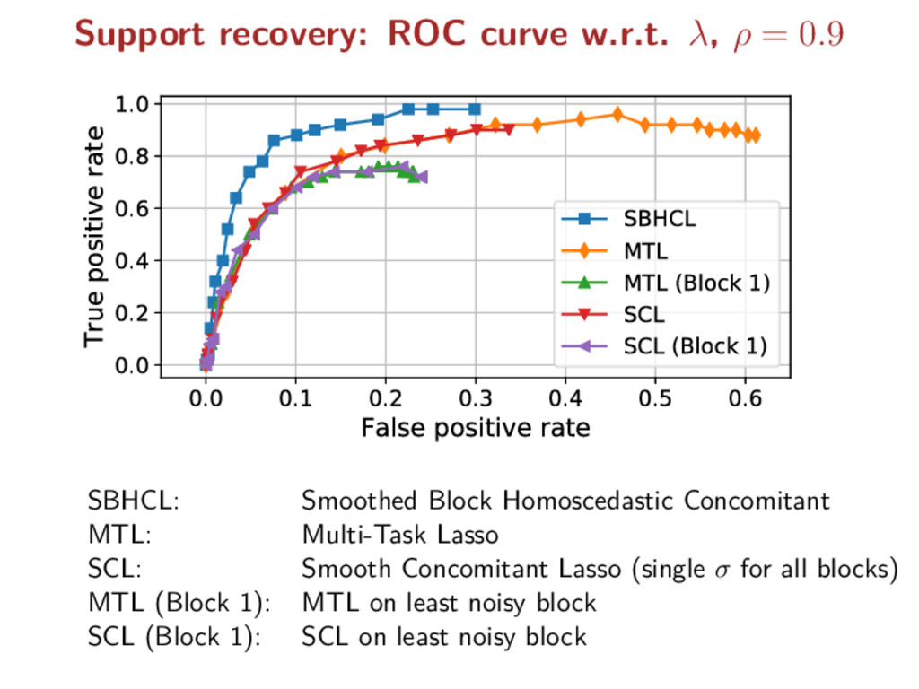
types of signals are recorded electrodes measure the electric potentials magnetometers measure the magnetic field gradiometers measure the gradient of the magnetic field = physical natures =⇒ different noise levels Key point: observations divided into 3 blocks but known partition!
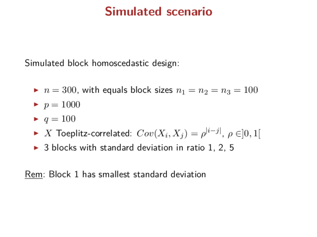
X = X1 . . . XK , Y = Y 1 . . . Y K , E = E1 . . . EK Σ∗ = diag(σ∗ 1 Idn1 , . . . , σ∗ K IdnK ) where n = n1 + · · · + nK For each block, the entries Ek i,j i.i.d. ∼ N(0, 1) (homoscedastic): Y k = XkB∗ + σ∗ k Ek MEG/EEG case: K = 3 corresponding to 3 physical signals 1) EEG, 2) MEG magnetometers, 3) MEG gradiometers
problem e.g., by Block Coordinate Descent (BCD) over rows, etc. Σ update: simply update the σk’s, potentially at each row Bj update (cheap : residuals are stored!)
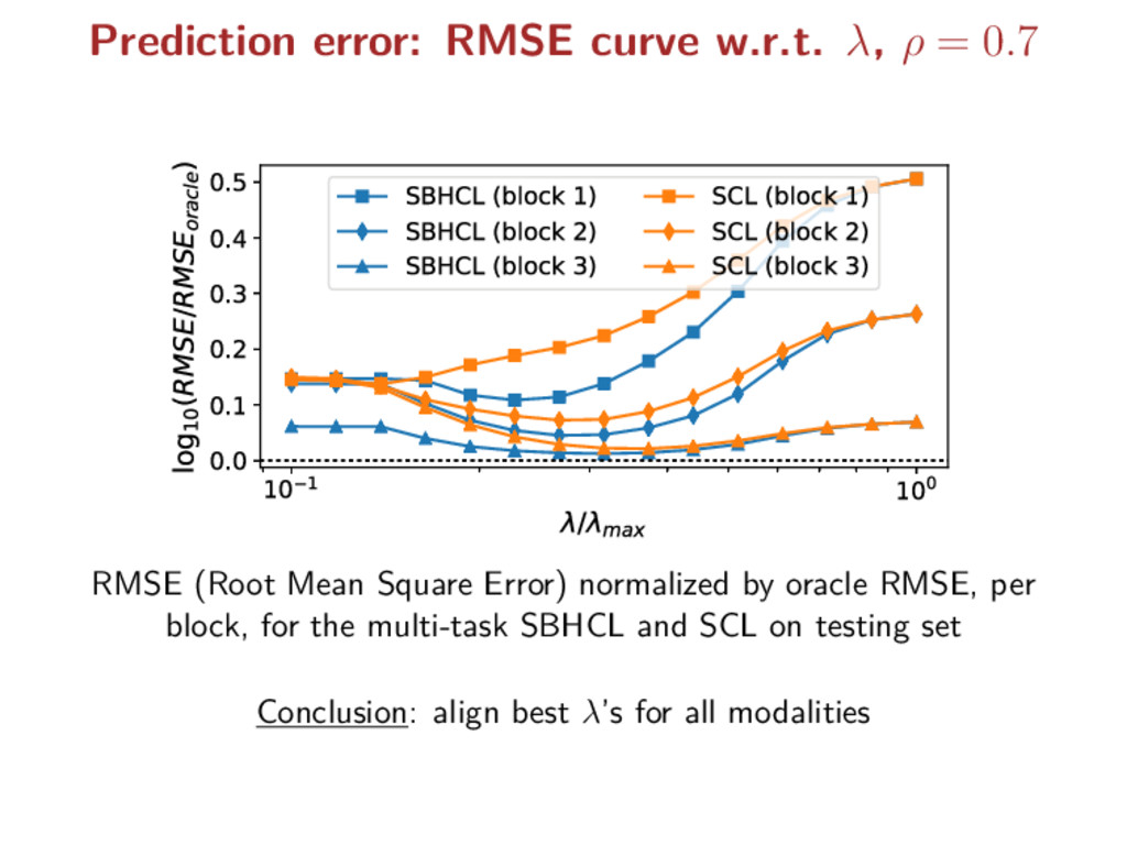
1 100 / max 0.0 0.1 0.2 0.3 0.4 0.5 log10 (RMSE/RMSEoracle ) SBHCL (block 1) SBHCL (block 2) SBHCL (block 3) SCL (block 1) SCL (block 2) SCL (block 3) RMSE (Root Mean Square Error) normalized by oracle RMSE, per block, for the multi-task SBHCL and SCL on testing set Conclusion: align best λ’s for all modalities
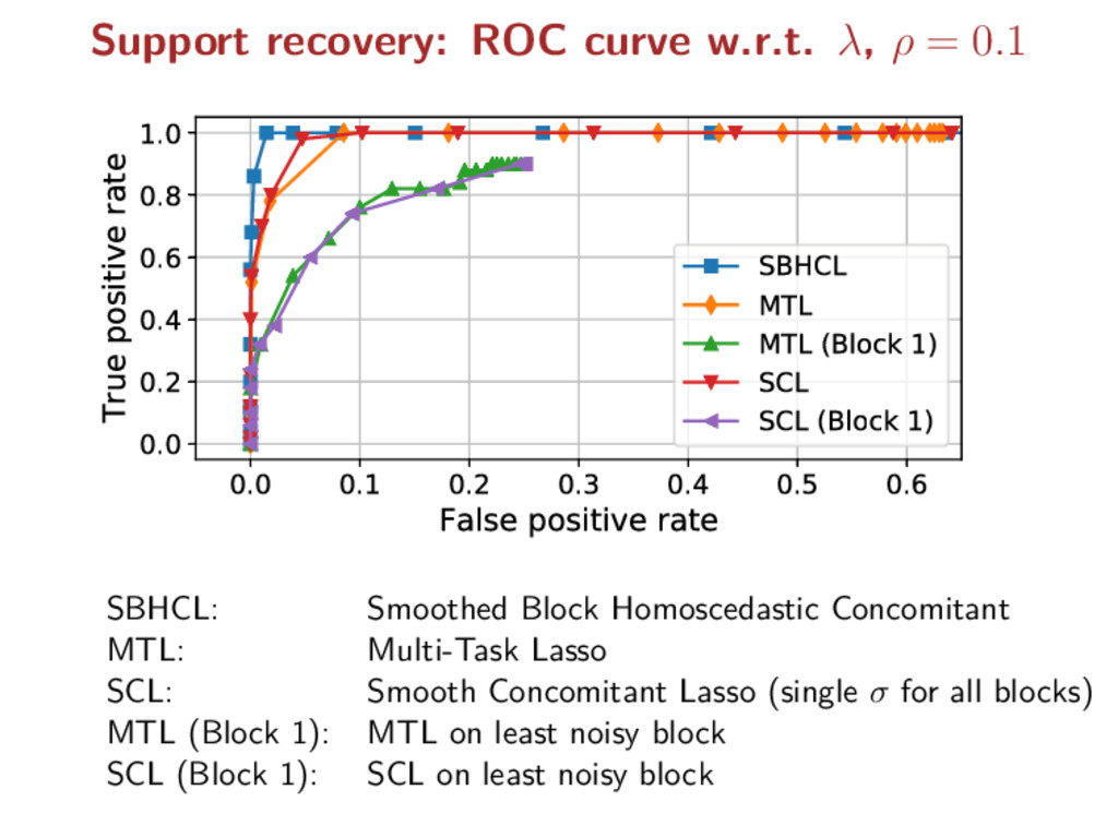
multi-task When“simple” noise structure known (e.g., block homoscedastic): cost equivalent to Multi-Task Lasso Handling multiple noise levels: helps both for prediction and support identification
multi-task When“simple” noise structure known (e.g., block homoscedastic): cost equivalent to Multi-Task Lasso Handling multiple noise levels: helps both for prediction and support identification Future work: non-convex penalties, other noise structures, etc.
multi-task When“simple” noise structure known (e.g., block homoscedastic): cost equivalent to Multi-Task Lasso Handling multiple noise levels: helps both for prediction and support identification Future work: non-convex penalties, other noise structures, etc.
open source implementation and good documentation so use those.” A. Gramfort Massias et al. (2018): to appear in AISTATS 2018 Python code is available at https://github.com/mathurinm/SHCL Powered with MooseTeX
systems. SIAM J. Comput., 24(2):227–234, 1995. D. Bertsimas, A. King, and R. Mazumder. Best subset selection via a modern optimization lens. Ann. Statist., 44(2):813–852, 2016. E. J. Candès, M. B. Wakin, and S. P. Boyd. Enhancing sparsity by reweighted l1 minimization. J. Fourier Anal. Applicat., 14(5-6):877–905, 2008. R. Tibshirani. Regression shrinkage and selection via the lasso. J. R. Stat. Soc. Ser. B Stat. Methodol., 58(1):267–288, 1996. S. S. Chen, D. L. Donoho, and M. A. Saunders. Atomic decomposition by basis pursuit. SIAM J. Sci. Comput., 20(1):33–61, 1998.
Joint covariate selection and joint subspace selection for multiple classification problems. Statistics and Computing, 20(2):231–252, 2010. P. J. Bickel, Y. Ritov, and A. B. Tsybakov. Simultaneous analysis of Lasso and Dantzig selector. Ann. Statist., 37(4):1705–1732, 2009. A. S. Dalalyan, M. Hebiri, and J. Lederer. On the prediction performance of the Lasso. Bernoulli, 23(1):552–581, 2017. D. L. Donoho and I. M. Johnstone. Adapting to unknown smoothness via wavelet shrinkage. J. Amer. Statist. Assoc., 90(432):1200–1224, 1995. T. Sun and C.-H. Zhang. Scaled sparse linear regression. Biometrika, 99(4):879–898, 2012.
Sons Inc., 1981. A. B. Owen. A robust hybrid of lasso and ridge regression. Contemporary Mathematics, 443:59–72, 2007. A. Belloni, V. Chernozhukov, and L. Wang. Square-root Lasso: pivotal recovery of sparse signals via conic programming. Biometrika, 98(4):791–806, 2011. Y. Nesterov. Smooth minimization of non-smooth functions. Math. Program., 103(1):127–152, 2005. E. Ndiaye, O. Fercoq, A. Gramfort, V. Leclère, and J. Salmon. Efficient smoothed concomitant Lasso estimation for high dimensional regression. In NCMIP, 2017.
order methods: A unified framework. SIAM J. Optim., 22(2):557–580, 2012. L. El Ghaoui, V. Viallon, and T. Rabbani. Safe feature elimination in sparse supervised learning. J. Pacific Optim., 8(4):667–698, 2012. E. Ndiaye, O. Fercoq, A. Gramfort, and J. Salmon. Gap safe screening rules for sparsity enforcing penalties. Technical report, 2016. R. Tibshirani, J. Bien, J. Friedman, T. J. Hastie, N. Simon, J. Taylor, and R. J. Tibshirani. Strong rules for discarding predictors in lasso-type problems. J. R. Stat. Soc. Ser. B Stat. Methodol., 74(2):245–266, 2012. T. B. Johnson and C. Guestrin. BLITZ: A principled meta-algorithm for scaling sparse optimization. In ICML, pages 1171–1179, 2015.