KTB-SSI.pdf

Transcript

1. A QUICK START GUIDE TO MACHINE LEARNING KEITH T. BUTLER 1
2. SOLID-STATE IONICS 2019 PYEONGCHANG SCIML/STFC/RAL ▸ Scientific machine learning group ▸ Interact with Facilities/Academia/Industry 2
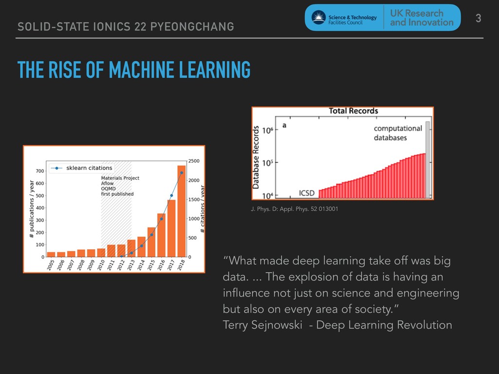
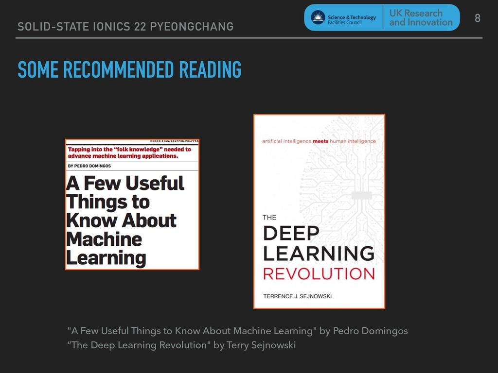
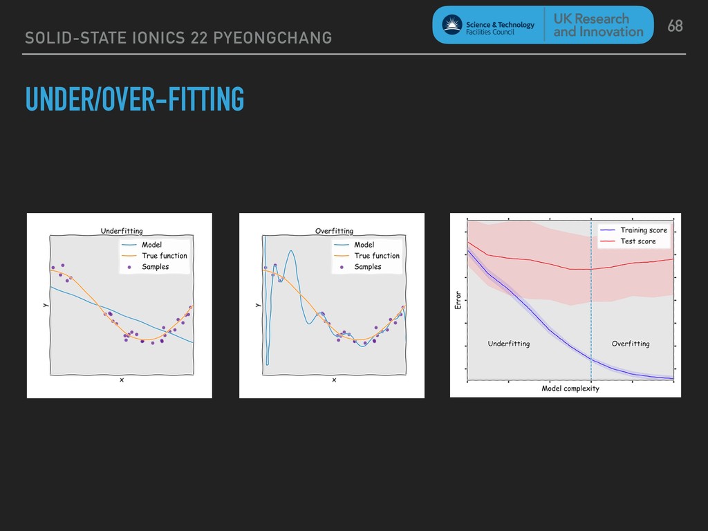
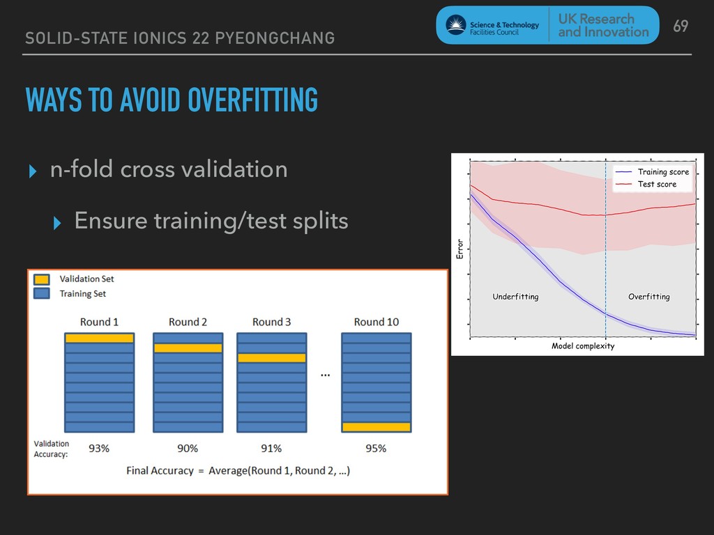
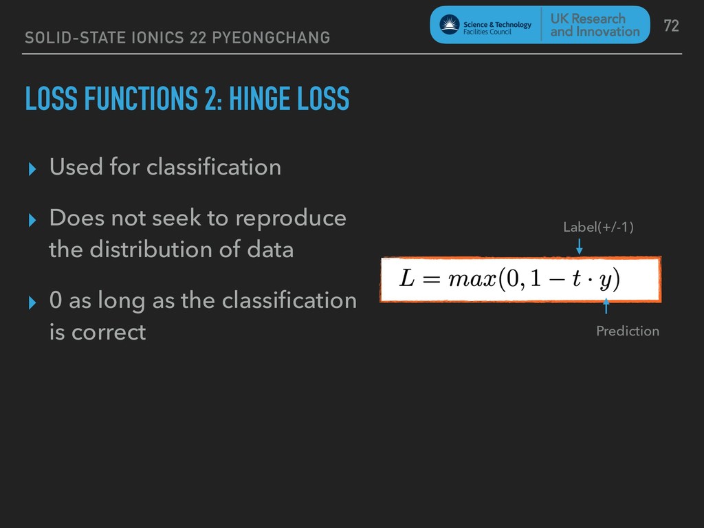
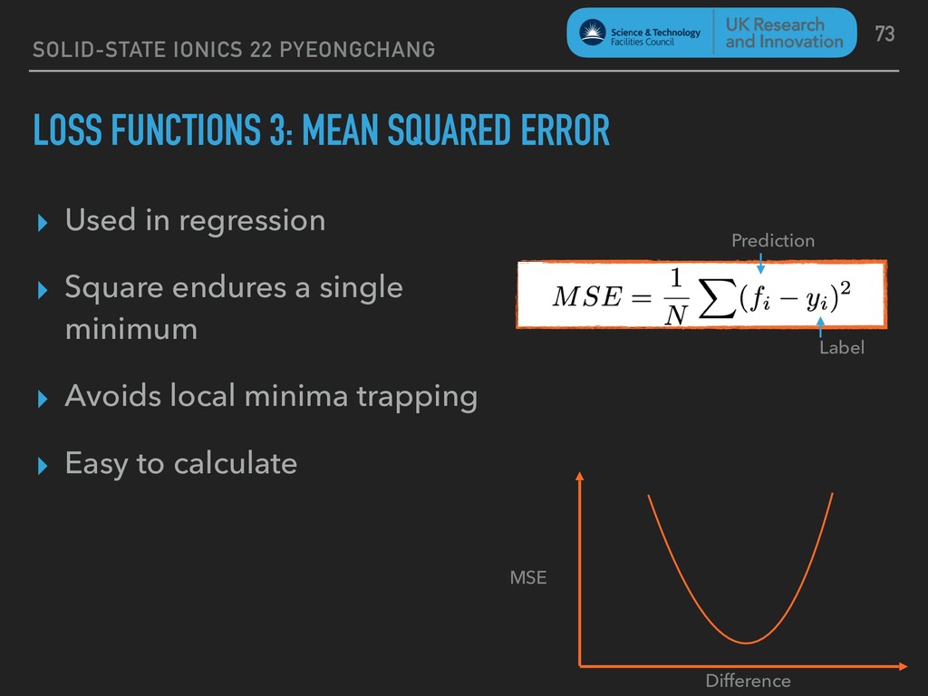
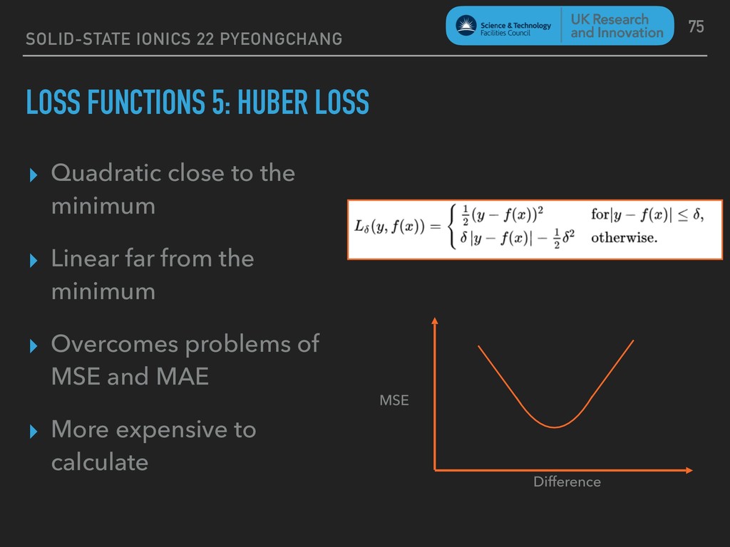
3. SOLID-STATE IONICS 22 PYEONGCHANG THE RISE OF MACHINE LEARNING 3 “What made deep learning take off was big data. ... The explosion of data is having an influence not just on science and engineering but also on every area of society.” Terry Sejnowski - Deep Learning Revolution J. Phys. D: Appl. Phys. 52 013001
4. SOLID-STATE IONICS 22 PYEONGCHANG ACADEMIA / INDUSTRY IN AI ▸ These companies all have many, very large, private datasets that they will never make publicly available ▸ Each of these companies employs many hundreds of computer scientists with PhDs in Machine Learning and AI ▸ Their researchers and developers have essentially unlimited computing power at their disposal 4
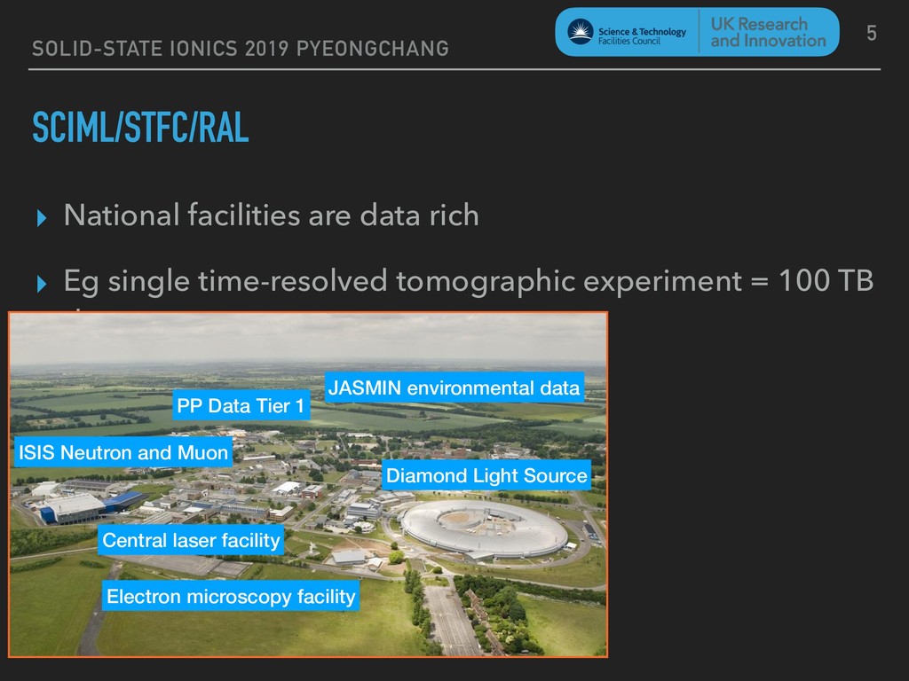
5. SOLID-STATE IONICS 2019 PYEONGCHANG SCIML/STFC/RAL ▸ National facilities are data rich ▸ Eg single time-resolved tomographic experiment = 100 TB data 5 Diamond Light Source ISIS Neutron and Muon Central laser facility Electron microscopy facility PP Data Tier 1 JASMIN environmental data
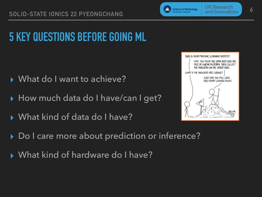
6. SOLID-STATE IONICS 22 PYEONGCHANG 5 KEY QUESTIONS BEFORE GOING ML ▸ What do I want to achieve? ▸ How much data do I have/can I get? ▸ What kind of data do I have? ▸ Do I care more about prediction or inference? ▸ What kind of hardware do I have? 6
7. SOLID-STATE IONICS 22 PYEONGCHANG TUTORIAL OVERVIEW ▸ An introduction to machine learning ▸ Background definitions ▸ Some traditional ML approaches ▸ Deep networks for materials science ▸ CNNs for images and spectra ▸ LSTMs for time series 7
8. SOLID-STATE IONICS 22 PYEONGCHANG SOME RECOMMENDED READING 8 "A Few Useful Things to Know About Machine Learning" by Pedro Domingos “The Deep Learning Revolution" by Terry Sejnowski
9. SOLID-STATE IONICS 22 PYEONGCHANG INTRODUCTION TO MACHINE LEARNING ▸ Some definitions ▸ Machine learning ▸ Some major issues ▸ Generalisation ▸ Representation ▸ Some popular algorithms (except neural nets!) ▸ Regression ▸ Bayes ▸ Decision trees 9
10. SOLID-STATE IONICS 22 PYEONGCHANG WHAT IS MACHINE LEARNING 10 ANIMALS LEARN FROM EXPERIENCE MACHINES ARE PROGRAMMED MACHINES LEARN FROM EXPERIENCE DATA
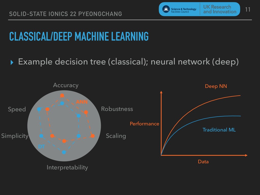
11. SOLID-STATE IONICS 22 PYEONGCHANG CLASSICAL/DEEP MACHINE LEARNING ▸ Example decision tree (classical); neural network (deep) 11 Robustness Scaling Interpretability Simplicity Speed Accuracy ANN DT Traditional ML Deep NN Performance Data
12. SOLID-STATE IONICS 22 PYEONGCHANG SUPERVISED/UNSUPERVISED ▸ Supervised learning ▸ Labelled training data ▸ Learn relations between input and label ▸ Unsupervised learning ▸ Unlabelled training data ▸ Learn relations between data points 12
13. SOLID-STATE IONICS 22 PYEONGCHANG CLASSIFICATION/REGRESSION ▸ Classification ▸ Separate data points ▸ Finite number of discreet classes ▸ Regression ▸ (Usually) a single value ▸ Infinite continuous variable 13
14. SOLID-STATE IONICS 22 PYEONGCHANG ONE-HOT ENCODING ▸ Classification problems ▸ Vector of length = number of categories ▸ Each element is the probability that the data represents a given class 14 Material Ortho Rhomb 1 0 0 1
15. SOLID-STATE IONICS 22 PYEONGCHANG PARAMETERS AND HYPER-PARAMETERS ▸ Parameters are part of the model ▸ E.g. y = Bx + C; B and C are parameters ▸ You do not set parameters ▸ Hyper-parameters control the learning process ▸ E.g. number of parameters allowed ▸ Type of optimiser ▸ Learning rate ▸ You do set hyper parameters 15
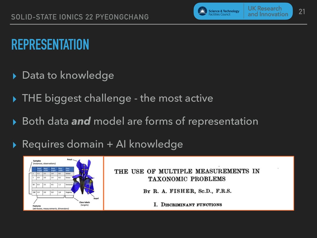
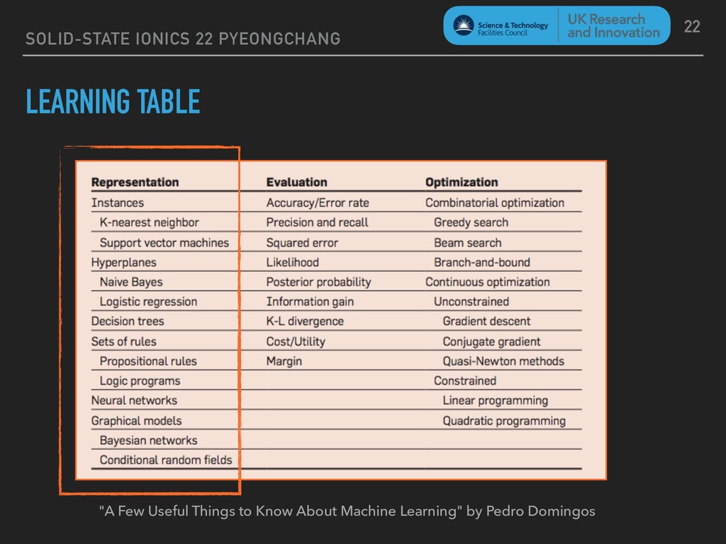
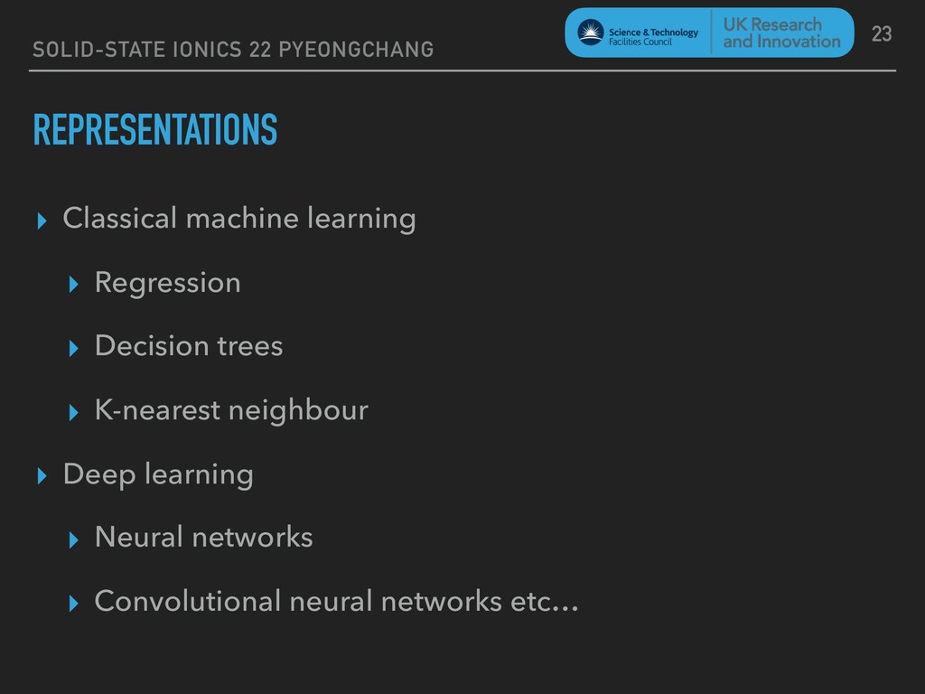
16. SOLID-STATE IONICS 22 PYEONGCHANG LEARNING Learning = Representation + Evaluation + Optimisation 16 ‣ Representation ‣ How we represent the knowledge. ‣ This also chooses the set of possible classifiers. ‣ Hypothesis space. ‣ Eg. Neural network, decision tree …
17. SOLID-STATE IONICS 22 PYEONGCHANG LEARNING Learning = Representation + Evaluation + Optimisation 17 ‣ Evaluation ‣ Objective function or scoring function. ‣ Distinguish good from bad classifiers. ‣ NB need not be the same as the external function that the classifier is optimising.
18. SOLID-STATE IONICS 22 PYEONGCHANG LEARNING Learning = Representation + Evaluation + Optimisation 18 ‣ Optimisation ‣ Searches between classifiers. ‣ Identifies the highest-scoring one. ‣ Determines the efficiency of a learner.
19. SOLID-STATE IONICS 22 PYEONGCHANG LEARNING Learning = Representation + Evaluation + Optimisation 19 ‣ Representation ‣ How we represent the knowledge. ‣ This also chooses the set of possible classifiers. ‣ Hypothesis space. ‣ Eg. Neural network, decision tree …
20. SOLID-STATE IONICS 22 PYEONGCHANG INDUCTION/REPRESENTATION ▸ Data alone is not enough – we need knowledge. 20
21. SOLID-STATE IONICS 22 PYEONGCHANG REPRESENTATION ▸ Data to knowledge ▸ THE biggest challenge - the most active ▸ Both data and model are forms of representation ▸ Requires domain + AI knowledge 21
22. SOLID-STATE IONICS 22 PYEONGCHANG LEARNING TABLE 22 "A Few Useful Things to Know About Machine Learning" by Pedro Domingos
23. SOLID-STATE IONICS 22 PYEONGCHANG REPRESENTATIONS ▸ Classical machine learning ▸ Regression ▸ Decision trees ▸ K-nearest neighbour ▸ Deep learning ▸ Neural networks ▸ Convolutional neural networks etc… 23
24. SOLID-STATE IONICS 22 PYEONGCHANG LINEAR REGRESSION 24 £20,000 £120,000 ? https://www.autodraw.com/
25. SOLID-STATE IONICS 22 PYEONGCHANG LINEAR REGRESSION 25 20k 120k 70k
26. SOLID-STATE IONICS 22 PYEONGCHANG NAIVE BAYES 26
27. SOLID-STATE IONICS 22 PYEONGCHANG NAIVE BAYES 27 Spam Not spam
28. SOLID-STATE IONICS 22 PYEONGCHANG NAIVE BAYES 28 Spam Not spam Cheap 80% chance that an email with the word ‘cheap’ will be spam
29. SOLID-STATE IONICS 22 PYEONGCHANG NAIVE BAYES 29 CHEAP PREGNENCY TEST Cheap Typos Caps title 80 % 60 % 90 % 99.2 %
30. SOLID-STATE IONICS 22 PYEONGCHANG DECISION TREES ▸ Has a band gap Y/N 30 At each node, the space is split such that samples with similar labels are grouped together
31. SOLID-STATE IONICS 22 PYEONGCHANG DECISION TREES 31 For a trial split at node j… The impurity of j is calculated for a trial split using an impurity function H()… And are chosen in a greedy fashion…
32. SOLID-STATE IONICS 22 PYEONGCHANG ENSEMBLE LEARNER ▸ Decision trees are weak learners ▸ A group of trees can overcome limitations ▸ Can optimise the group or chose randomly ▸ Random forest ▸ Gradient boosted 32
33. SOLID-STATE IONICS 22 PYEONGCHANG EXAMPLE: GRADIENT BOOSTED 33 + + Root mean squared error (RMSE) Sub model of errors Learning rate …
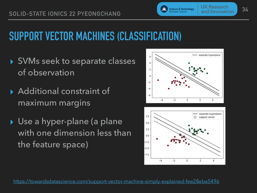
34. SOLID-STATE IONICS 22 PYEONGCHANG SUPPORT VECTOR MACHINES (CLASSIFICATION) ▸ SVMs seek to separate classes of observation ▸ Additional constraint of maximum margins ▸ Use a hyper-plane (a plane with one dimension less than the feature space) 34 https://towardsdatascience.com/support-vector-machine-simply-explained-fee28eba5496
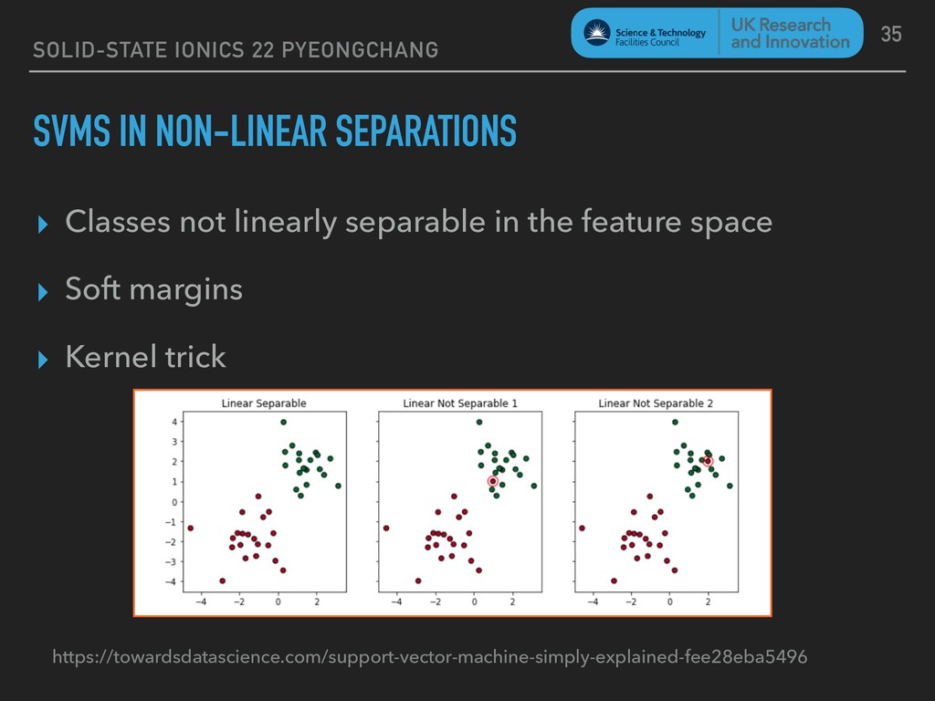
35. SOLID-STATE IONICS 22 PYEONGCHANG SVMS IN NON-LINEAR SEPARATIONS ▸ Classes not linearly separable in the feature space ▸ Soft margins ▸ Kernel trick 35 https://towardsdatascience.com/support-vector-machine-simply-explained-fee28eba5496
36. SOLID-STATE IONICS 22 PYEONGCHANG SVMS WITH SOFT MARGINS ▸ Tolerate a certain number of mis-classifications to maximise the margin ▸ Trade-off between mis-classification and margin width ▸ Tolerance hyper-parameter determines the balance 36 Classification is more important than margin Margin is more important than classification
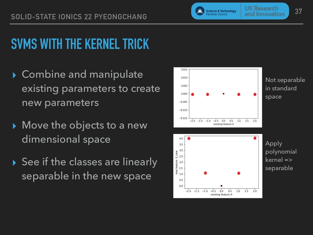
37. SOLID-STATE IONICS 22 PYEONGCHANG SVMS WITH THE KERNEL TRICK ▸ Combine and manipulate existing parameters to create new parameters ▸ Move the objects to a new dimensional space ▸ See if the classes are linearly separable in the new space 37 Not separable in standard space Apply polynomial kernel => separable
38. SOLID-STATE IONICS 22 PYEONGCHANG CLASSICAL MODELS SUMMARY 38
39. SOLID-STATE IONICS 22 PYEONGCHANG NEURAL NETWORKS ▸ A history of neural nets ▸ Rise-Fall-Rise-Fall-Rise-? ▸ The elements of a network ▸ Neurons, connections, optimisers ▸ Modern networks: CNNs ▸ Image recognition, feature detection etc 39
40. SOLID-STATE IONICS 22 PYEONGCHANG THE PERCEPTRON ▸ Originally a device ▸ Intended for binary classification ▸ Produces a single output from a matrix of inputs, weights and biases 40
41. SOLID-STATE IONICS 22 PYEONGCHANG THE FIRST FALL OF NEURAL NETWORKS ▸ Single layer ▸ Minsky and Papert showed they could not solve non-linear classification 41
42. SOLID-STATE IONICS 22 PYEONGCHANG THE NEXT WAVE OF NEURAL NETS: 1980S ▸ Back propagation ▸ Now gradients could be used to minimise error ▸ Modifications back propagate through the network using the chain rule 42
43. SOLID-STATE IONICS 22 PYEONGCHANG THE NEXT WAVE OF NEURAL NETS: 1980S ▸ Multi-layer perceptrons (MLPs) ▸ Can now solve non-linear problems 43
44. SOLID-STATE IONICS 22 PYEONGCHANG THE ELEMENTS OF A NEURAL NETWORK ▸ Input layer ▸ Hidden layers ▸ Output layer 44
45. SOLID-STATE IONICS 22 PYEONGCHANG THE ELEMENTS OF A NEURAL NETWORK ▸ Input layer ▸ Hidden layers ▸ Output layer 45 ‣ Data structure ‣ Features of the data
46. SOLID-STATE IONICS 22 PYEONGCHANG THE ELEMENTS OF A NEURAL NETWORK ▸ Input layer ▸ Hidden layers ▸ Output layer 46 ‣ Regression ‣ Single unit (usually) ‣ Classification ‣ Multiple units ‣ One-hot encoding
47. SOLID-STATE IONICS 22 PYEONGCHANG HIDDEN LAYERS ▸ Neurons ▸ Connections 47 Outputs from previous Matrix of weights Bias Activation function Signal to next layer
48. SOLID-STATE IONICS 22 PYEONGCHANG BACK PROPAGATION ▸ Learn from the loss 48 LOSS(L) y[1] y[2] y[l] dy[l] Notation: dL/dy[l] => dy[l] dy[1] dy[2] dw[1] db[1] dw[2] db[2] dw[l] db[l] y[0]
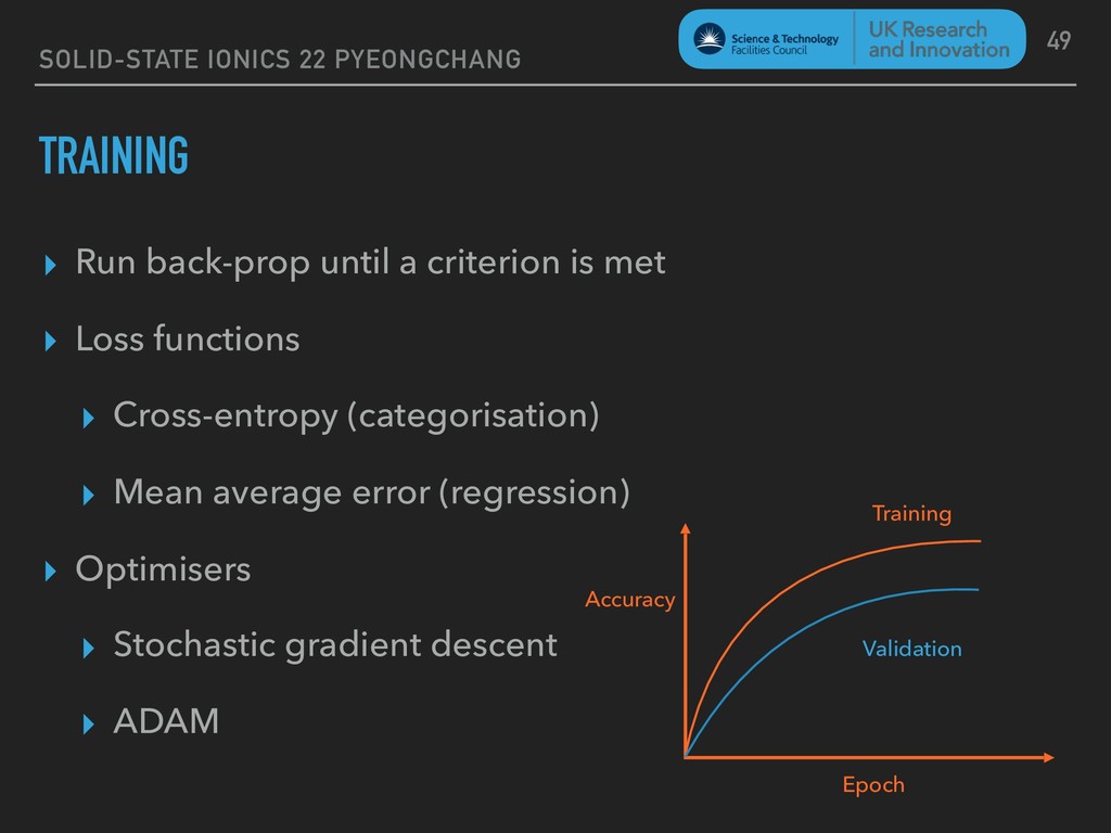
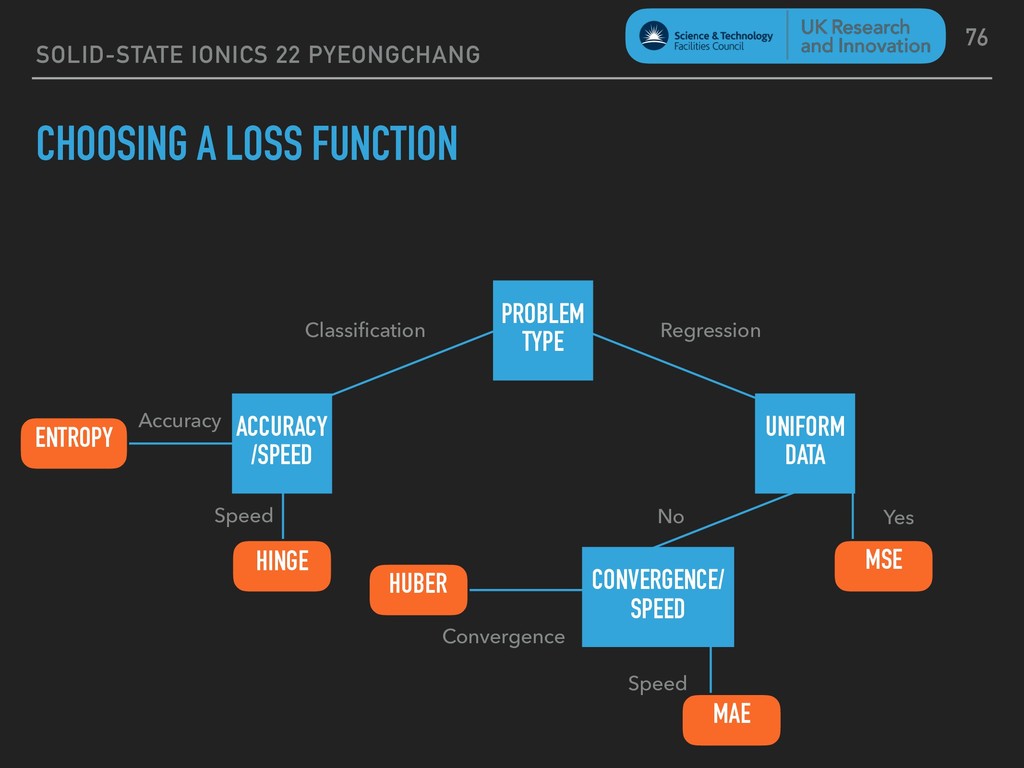
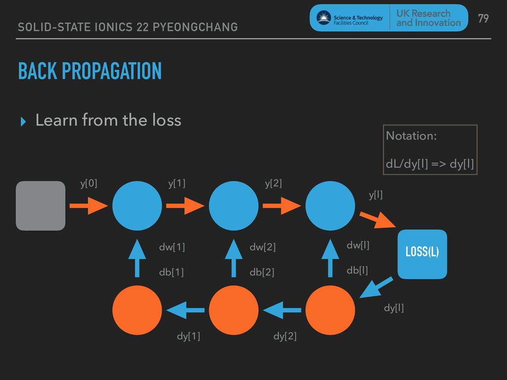
49. SOLID-STATE IONICS 22 PYEONGCHANG TRAINING ▸ Run back-prop until a criterion is met ▸ Loss functions ▸ Cross-entropy (categorisation) ▸ Mean average error (regression) ▸ Optimisers ▸ Stochastic gradient descent ▸ ADAM 49 Validation Training Accuracy Epoch
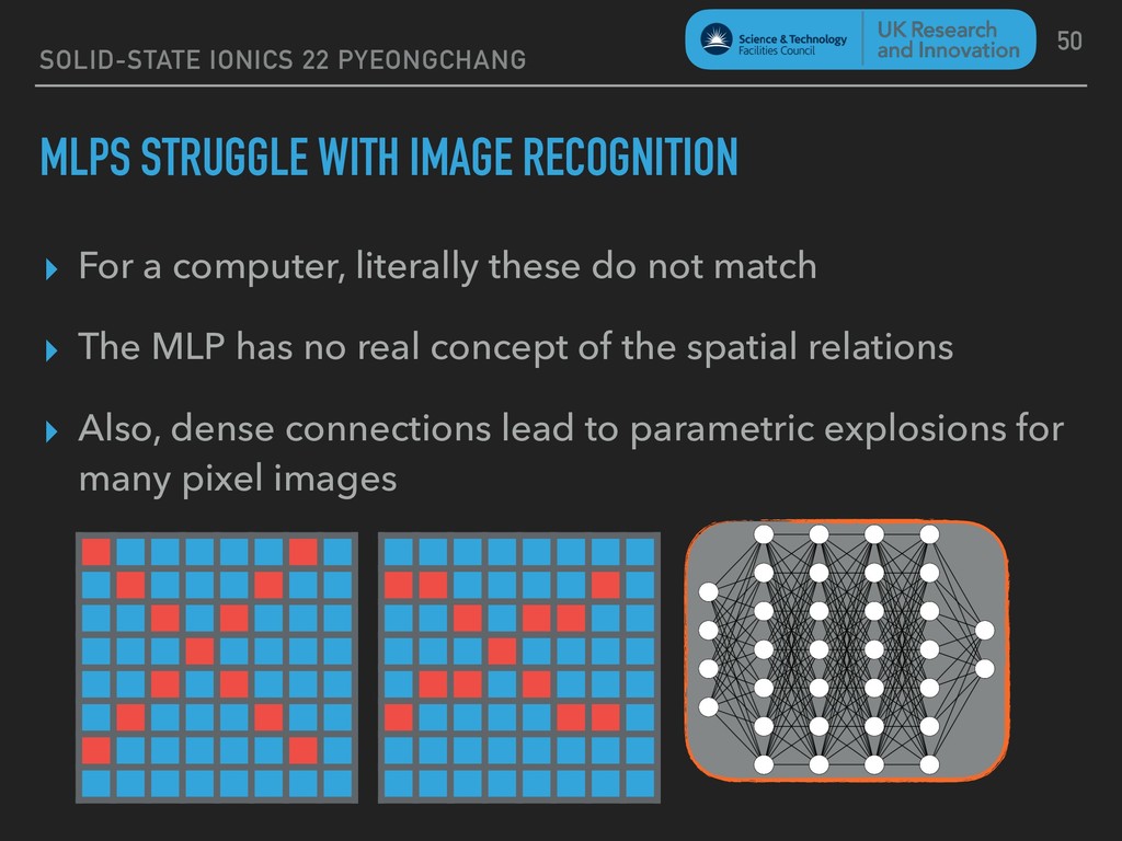
50. SOLID-STATE IONICS 22 PYEONGCHANG MLPS STRUGGLE WITH IMAGE RECOGNITION ▸ For a computer, literally these do not match ▸ The MLP has no real concept of the spatial relations ▸ Also, dense connections lead to parametric explosions for many pixel images 50
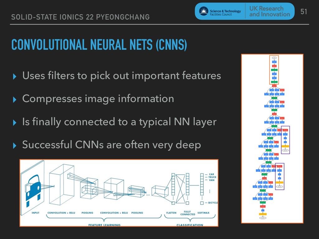
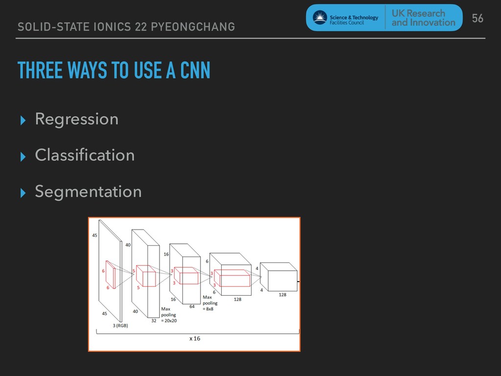
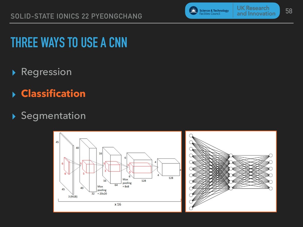
51. SOLID-STATE IONICS 22 PYEONGCHANG CONVOLUTIONAL NEURAL NETS (CNNS) ▸ Uses filters to pick out important features ▸ Compresses image information ▸ Is finally connected to a typical NN layer ▸ Successful CNNs are often very deep 51
52. SOLID-STATE IONICS 22 PYEONGCHANG HOW CNNS WORK ▸ Filters work to pick out features in the image 52 0.8 1 1 0.5 1 1 0.8 =
53. SOLID-STATE IONICS 22 PYEONGCHANG HOW CNNS WORK ▸ Filter is a matrix ▸ Filter dot product with image to produce scalar ▸ A number of filters are added at each layer 53 5x5 Filter 32x32 image 28x28 image
54. SOLID-STATE IONICS 22 PYEONGCHANG LOOKING AT THE FILTERS ▸ Visualise trained filters to see what they detect ▸ Example form the AlexNet network ▸ Filters pick up edges and colours 54
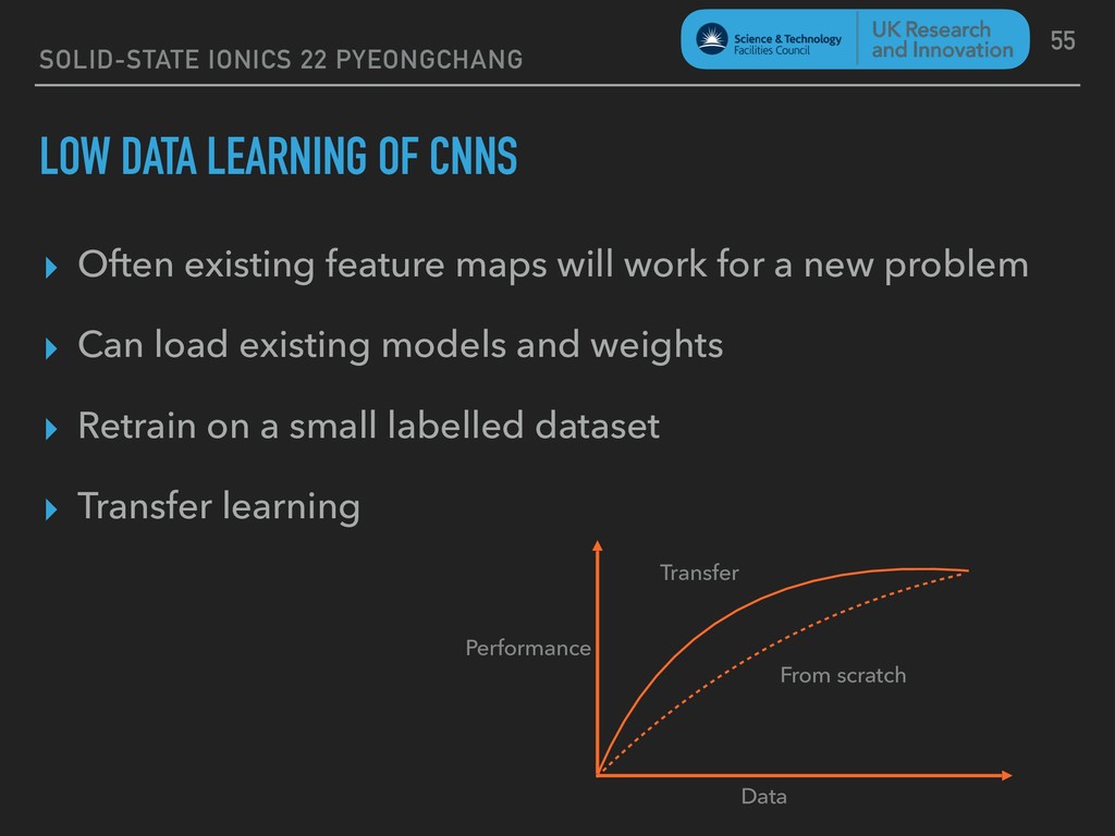
55. SOLID-STATE IONICS 22 PYEONGCHANG LOW DATA LEARNING OF CNNS ▸ Often existing feature maps will work for a new problem ▸ Can load existing models and weights ▸ Retrain on a small labelled dataset ▸ Transfer learning 55 Performance Data From scratch Transfer
56. SOLID-STATE IONICS 22 PYEONGCHANG THREE WAYS TO USE A CNN ▸ Regression ▸ Classification ▸ Segmentation 56
57. SOLID-STATE IONICS 22 PYEONGCHANG THREE WAYS TO USE A CNN ▸ Regression ▸ Classification ▸ Segmentation 57
58. SOLID-STATE IONICS 22 PYEONGCHANG THREE WAYS TO USE A CNN ▸ Regression ▸ Classification ▸ Segmentation 58
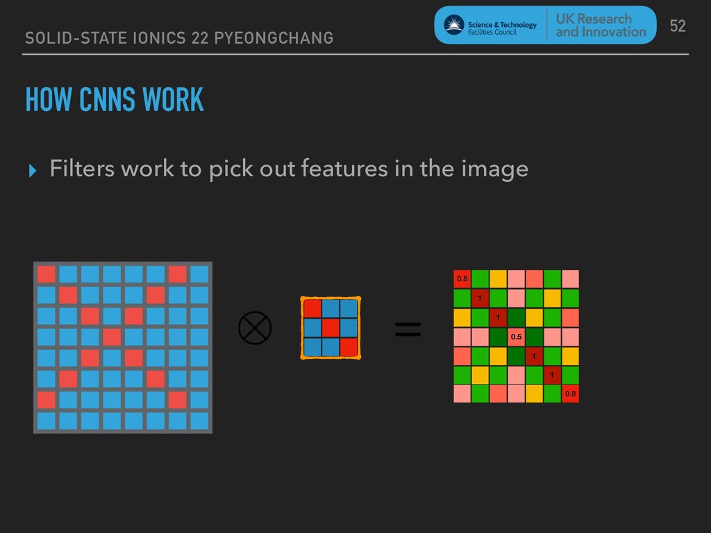
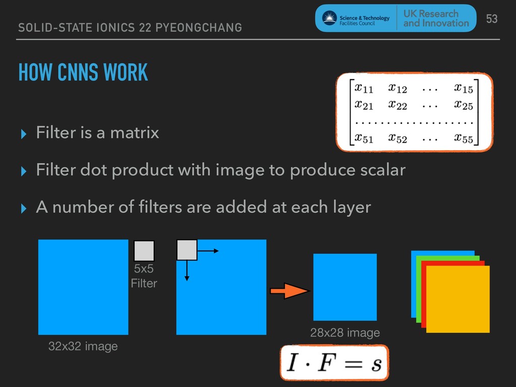
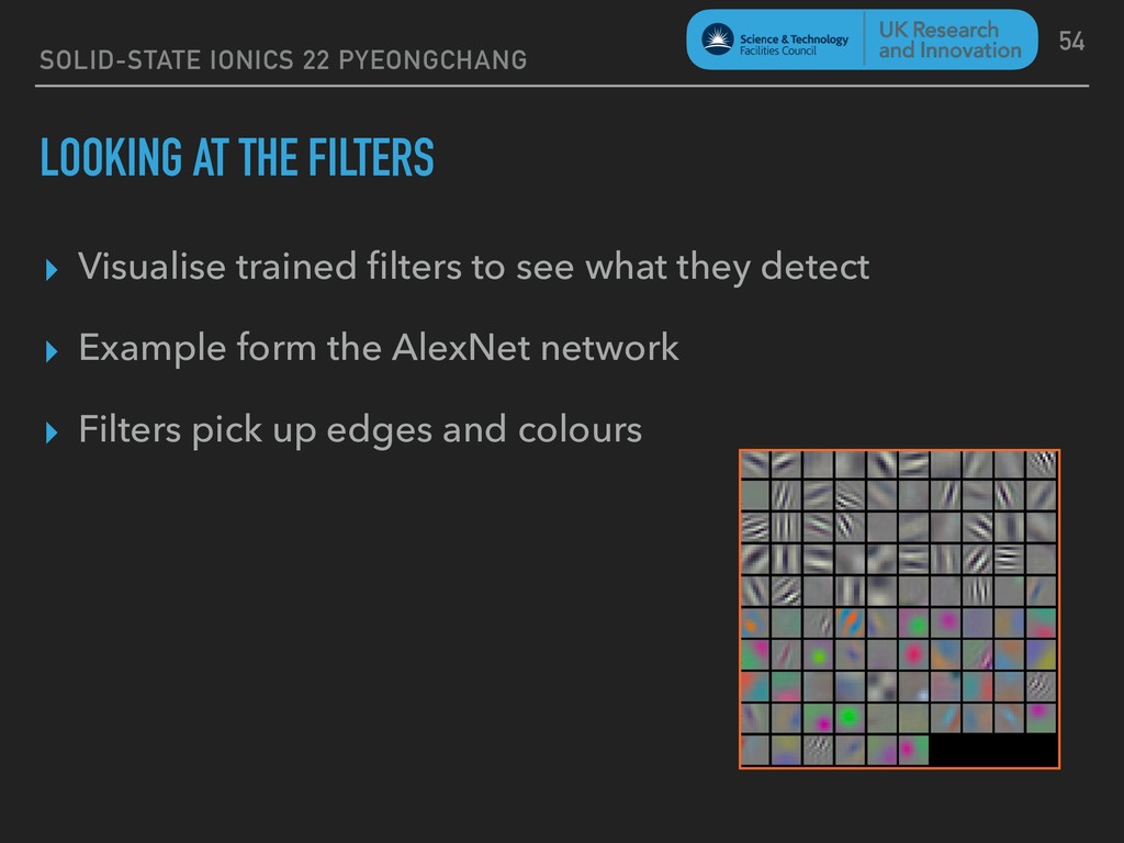
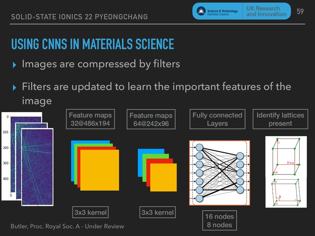
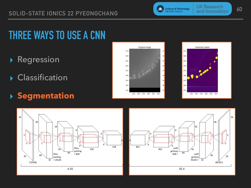
59. SOLID-STATE IONICS 22 PYEONGCHANG USING CNNS IN MATERIALS SCIENCE ▸ Images are compressed by filters ▸ Filters are updated to learn the important features of the image 59 Feature maps 32@486x194 3x3 kernel Feature maps 64@242x96 3x3 kernel Fully connected Layers 16 nodes 8 nodes Identify lattices present Butler, Proc. Royal Soc. A - Under Review
60. SOLID-STATE IONICS 22 PYEONGCHANG THREE WAYS TO USE A CNN ▸ Regression ▸ Classification ▸ Segmentation 60
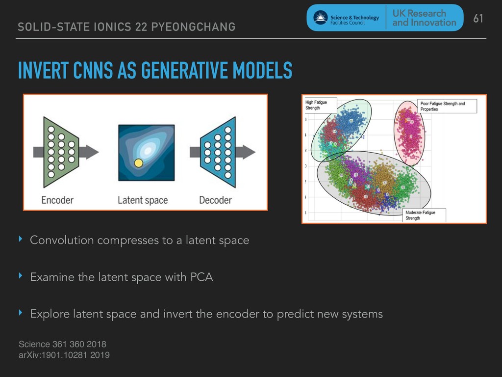
61. SOLID-STATE IONICS 22 PYEONGCHANG INVERT CNNS AS GENERATIVE MODELS ‣ Convolution compresses to a latent space ‣ Examine the latent space with PCA ‣ Explore latent space and invert the encoder to predict new systems 61 Science 361 360 2018 arXiv:1901.10281 2019
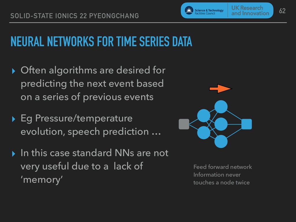
62. SOLID-STATE IONICS 22 PYEONGCHANG NEURAL NETWORKS FOR TIME SERIES DATA ▸ Often algorithms are desired for predicting the next event based on a series of previous events ▸ Eg Pressure/temperature evolution, speech prediction … ▸ In this case standard NNs are not very useful due to a lack of ‘memory’ 62 Feed forward network Information never touches a node twice
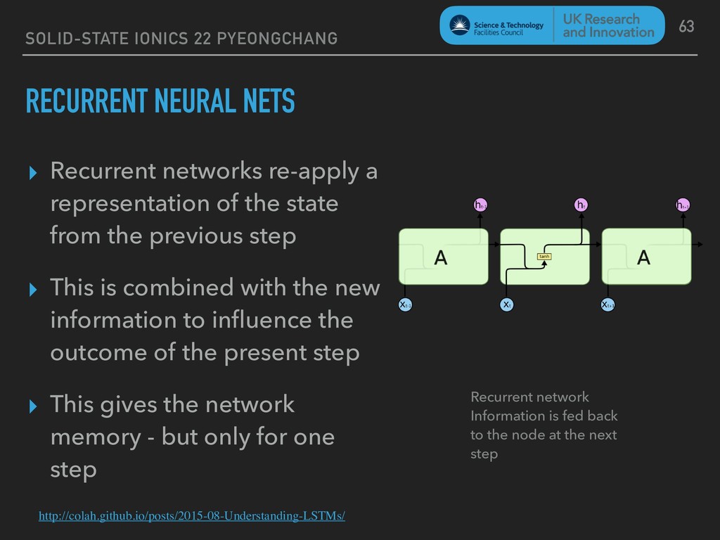
63. SOLID-STATE IONICS 22 PYEONGCHANG RECURRENT NEURAL NETS ▸ Recurrent networks re-apply a representation of the state from the previous step ▸ This is combined with the new information to influence the outcome of the present step ▸ This gives the network memory - but only for one step 63 Recurrent network Information is fed back to the node at the next step http://colah.github.io/posts/2015-08-Understanding-LSTMs/
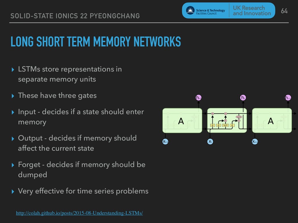
64. SOLID-STATE IONICS 22 PYEONGCHANG LONG SHORT TERM MEMORY NETWORKS ▸ LSTMs store representations in separate memory units ▸ These have three gates ▸ Input - decides if a state should enter memory ▸ Output - decides if memory should affect the current state ▸ Forget - decides if memory should be dumped ▸ Very effective for time series problems 64 http://colah.github.io/posts/2015-08-Understanding-LSTMs/
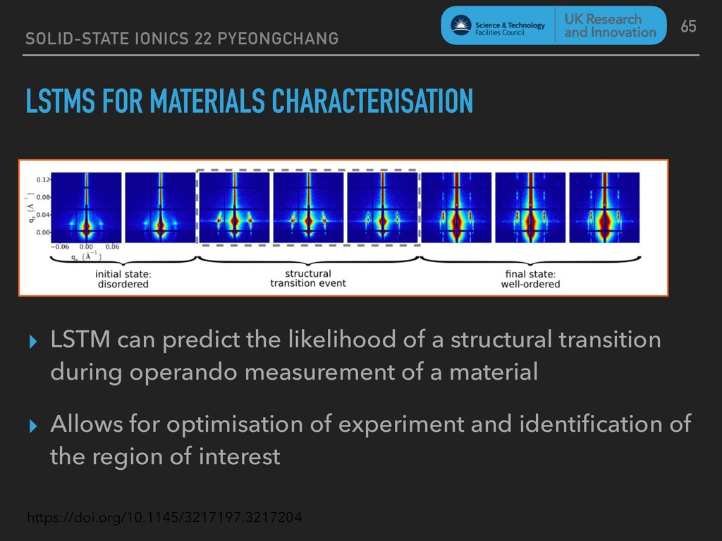
65. SOLID-STATE IONICS 22 PYEONGCHANG LSTMS FOR MATERIALS CHARACTERISATION ▸ LSTM can predict the likelihood of a structural transition during operando measurement of a material ▸ Allows for optimisation of experiment and identification of the region of interest 65 https://doi.org/10.1145/3217197.3217204
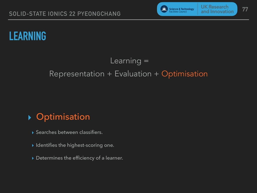
66. SOLID-STATE IONICS 22 PYEONGCHANG LEARNING Learning = Representation + Evaluation + Optimisation 66 ‣ Evaluation ‣ Objective function or scoring function. ‣ Distinguish good from bad classifiers. ‣ NB need not be the same as the external function that the classifier is optimising.
67. SOLID-STATE IONICS 22 PYEONGCHANG OVER/UNDERFITTING ▸ Bias ▸ Constantly learning the same wrong thing. ▸ Variance ▸ Learn random things irrespective of real values. 67
68. SOLID-STATE IONICS 22 PYEONGCHANG UNDER/OVER-FITTING 68
69. SOLID-STATE IONICS 22 PYEONGCHANG WAYS TO AVOID OVERFITTING ▸ n-fold cross validation ▸ Ensure training/test splits 69
70. SOLID-STATE IONICS 22 PYEONGCHANG EVALUATION OF MODELS : LOSS FUNCTIONS ▸ Objective function = loss function = cost function ▸ Must faithfully represent the “goodness” of a model in a single number 70
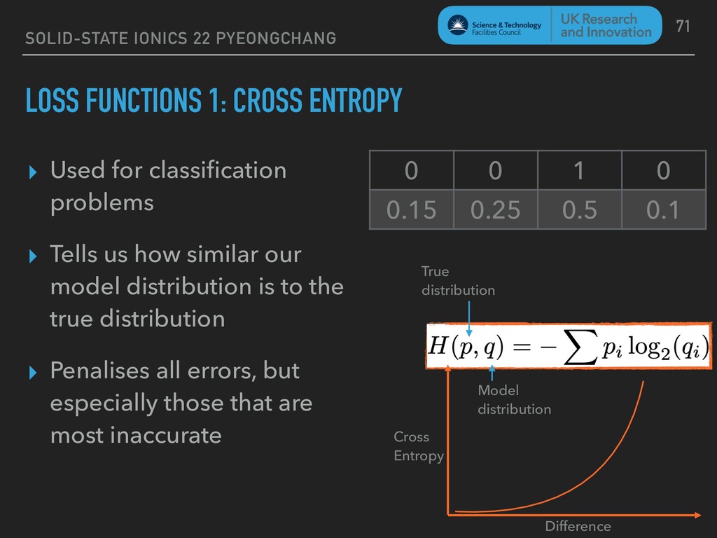
71. SOLID-STATE IONICS 22 PYEONGCHANG LOSS FUNCTIONS 1: CROSS ENTROPY ▸ Used for classification problems ▸ Tells us how similar our model distribution is to the true distribution ▸ Penalises all errors, but especially those that are most inaccurate 71 Difference Cross Entropy True distribution Model distribution 0 0 1 0 0.15 0.25 0.5 0.1
72. SOLID-STATE IONICS 22 PYEONGCHANG LOSS FUNCTIONS 2: HINGE LOSS ▸ Used for classification ▸ Does not seek to reproduce the distribution of data ▸ 0 as long as the classification is correct 72 Label(+/-1) Prediction
73. SOLID-STATE IONICS 22 PYEONGCHANG LOSS FUNCTIONS 3: MEAN SQUARED ERROR ▸ Used in regression ▸ Square endures a single minimum ▸ Avoids local minima trapping ▸ Easy to calculate 73 Difference MSE Prediction Label
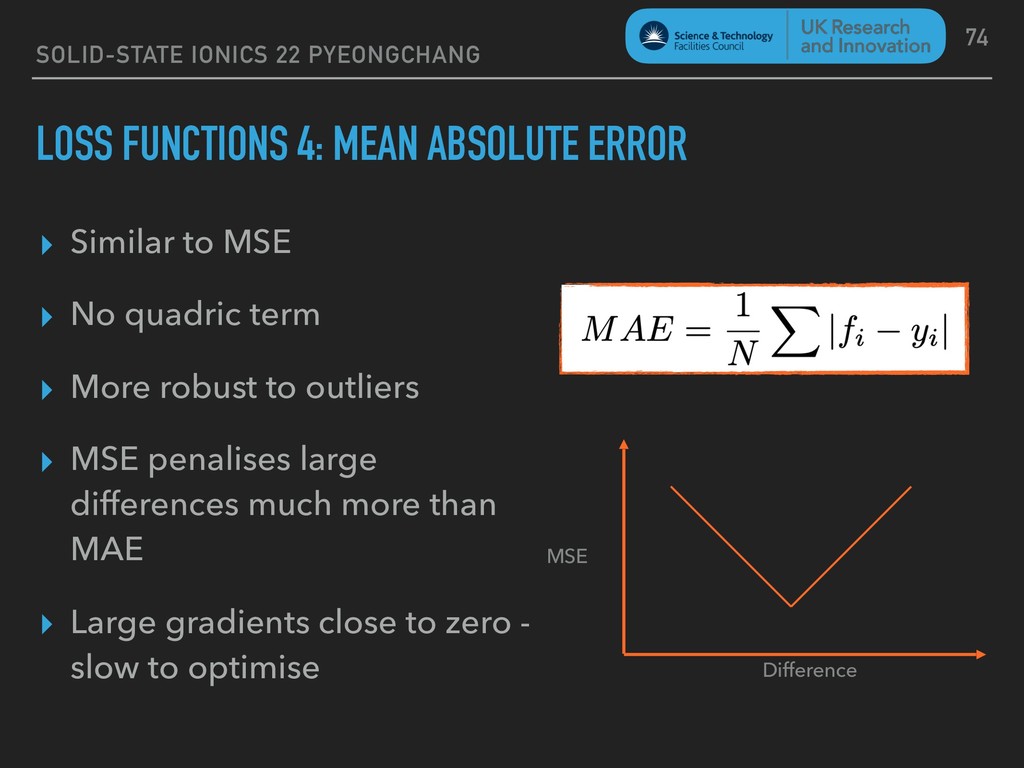
74. SOLID-STATE IONICS 22 PYEONGCHANG LOSS FUNCTIONS 4: MEAN ABSOLUTE ERROR ▸ Similar to MSE ▸ No quadric term ▸ More robust to outliers ▸ MSE penalises large differences much more than MAE ▸ Large gradients close to zero - slow to optimise 74 Difference MSE
75. SOLID-STATE IONICS 22 PYEONGCHANG LOSS FUNCTIONS 5: HUBER LOSS ▸ Quadratic close to the minimum ▸ Linear far from the minimum ▸ Overcomes problems of MSE and MAE ▸ More expensive to calculate 75 Difference MSE
76. SOLID-STATE IONICS 22 PYEONGCHANG CHOOSING A LOSS FUNCTION 76 PROBLEM TYPE ACCURACY /SPEED UNIFORM DATA CONVERGENCE/ SPEED Classification Regression Yes No Convergence Speed MSE MAE HUBER HINGE ENTROPY Speed Accuracy
77. SOLID-STATE IONICS 22 PYEONGCHANG LEARNING Learning = Representation + Evaluation + Optimisation 77 ‣ Optimisation ‣ Searches between classifiers. ‣ Identifies the highest-scoring one. ‣ Determines the efficiency of a learner.
78. SOLID-STATE IONICS 22 PYEONGCHANG OPTIMISERS ▸ Maximise/minimise an objective function ▸ In our case the loss function ▸ Updates the weight and biases 78
79. SOLID-STATE IONICS 22 PYEONGCHANG BACK PROPAGATION ▸ Learn from the loss 79 LOSS(L) y[1] y[2] y[l] dy[l] Notation: dL/dy[l] => dy[l] dy[1] dy[2] dw[1] db[1] dw[2] db[2] dw[l] db[l] y[0]
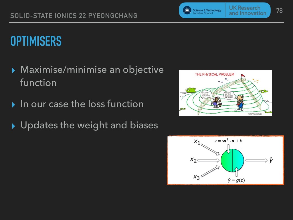
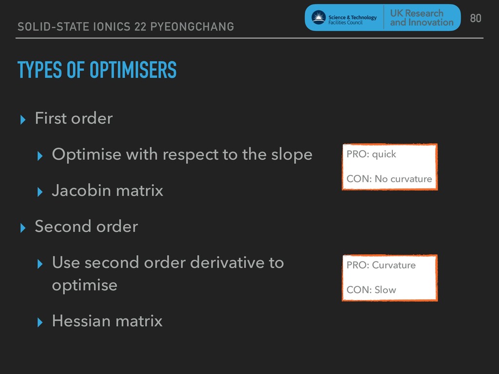
80. SOLID-STATE IONICS 22 PYEONGCHANG TYPES OF OPTIMISERS ▸ First order ▸ Optimise with respect to the slope ▸ Jacobin matrix ▸ Second order ▸ Use second order derivative to optimise ▸ Hessian matrix 80 PRO: quick CON: No curvature PRO: Curvature CON: Slow
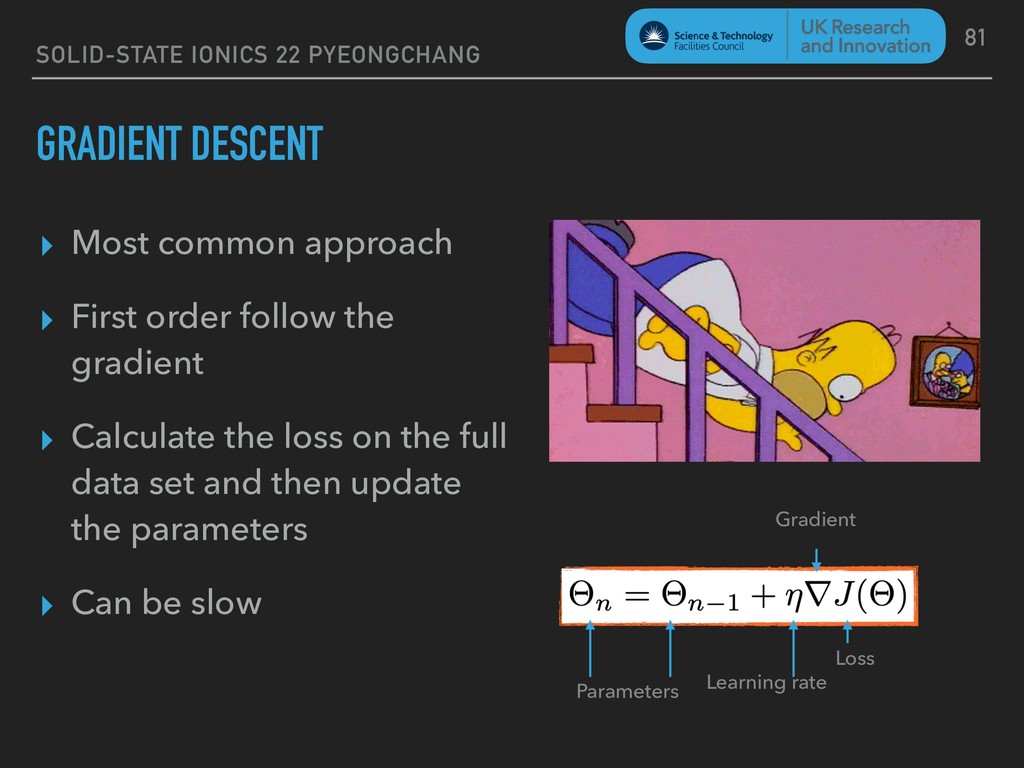
81. SOLID-STATE IONICS 22 PYEONGCHANG GRADIENT DESCENT ▸ Most common approach ▸ First order follow the gradient ▸ Calculate the loss on the full data set and then update the parameters ▸ Can be slow 81 Loss Parameters Learning rate Gradient
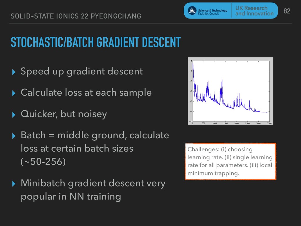
82. SOLID-STATE IONICS 22 PYEONGCHANG STOCHASTIC/BATCH GRADIENT DESCENT ▸ Speed up gradient descent ▸ Calculate loss at each sample ▸ Quicker, but noisey ▸ Batch = middle ground, calculate loss at certain batch sizes (~50-256) ▸ Minibatch gradient descent very popular in NN training 82 Challenges: (i) choosing learning rate. (ii) single learning rate for all parameters. (iii) local minimum trapping.
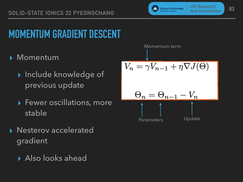
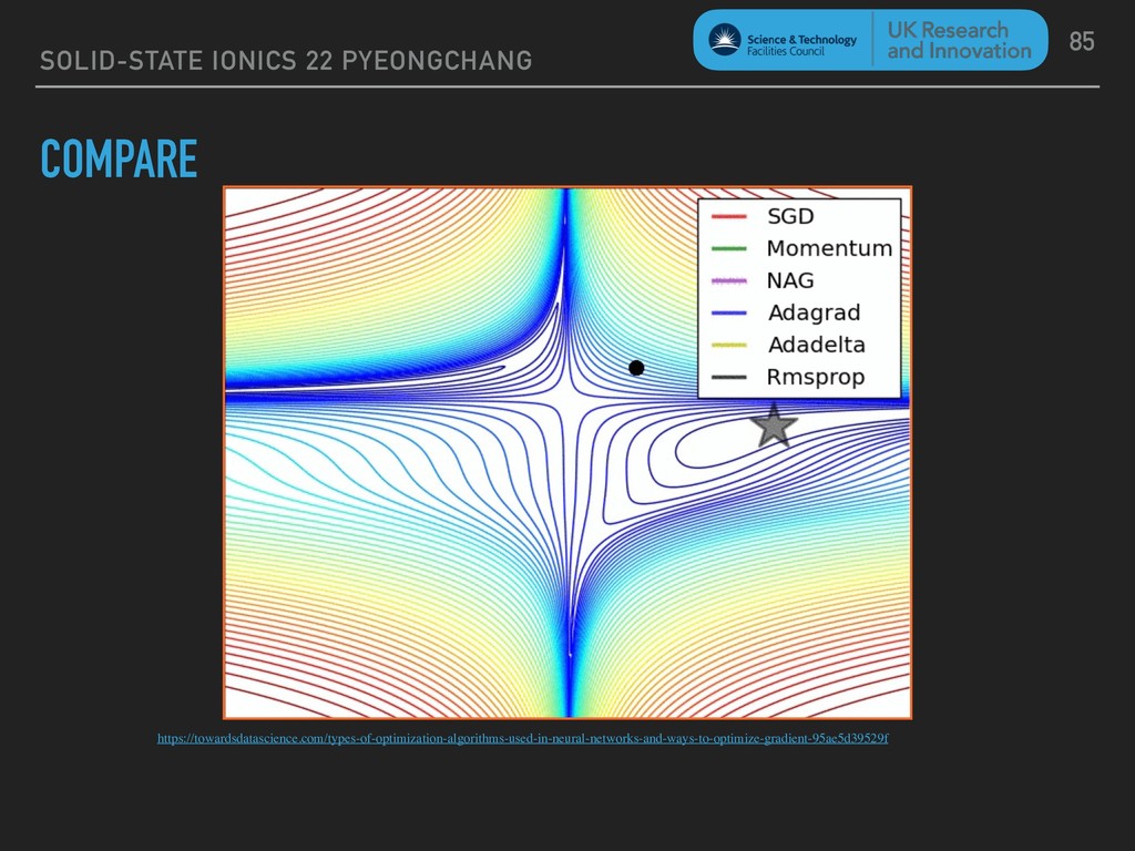
83. SOLID-STATE IONICS 22 PYEONGCHANG MOMENTUM GRADIENT DESCENT ▸ Momentum ▸ Include knowledge of previous update ▸ Fewer oscillations, more stable ▸ Nesterov accelerated gradient ▸ Also looks ahead 83 Parameters Update Momentum term
84. SOLID-STATE IONICS 22 PYEONGCHANG ADAPTIVE MOMENTUM ▸ Allows the learning rate to adjust for parameters ▸ Small updates for frequent parameters, large updates for sparse parameters ▸ Adagrad, Adadelta, Adam ▸ Adam is becoming the most popular method for NN optimisation 84
85. SOLID-STATE IONICS 22 PYEONGCHANG COMPARE 85 https://towardsdatascience.com/types-of-optimization-algorithms-used-in-neural-networks-and-ways-to-optimize-gradient-95ae5d39529f
86. SOLID-STATE IONICS 22 PYEONGCHANG USEFUL LINKS ▸ Blog on types of machine learning: https:// machinelearningmastery.com/a-tour-of-machine-learning- algorithms/ ▸ Open source reading on many ML issues: https://distill.pub/ ▸ Information about back-propagation: https:// www.youtube.com/watch?v=Ilg3gGewQ5U ▸ More on CNNs: https://towardsdatascience.com/a- comprehensive-guide-to-convolutional-neural-networks-the- eli5-way-3bd2b1164a53 86
87. SOLID-STATE IONICS 22 PYEONGCHANG SUMMARY ▸ Understanding your problem before diving in is critical ▸ Understand your data ▸ Traditional methods work well on well structured and characterised datasets ▸ CNNs are useful for analysis of patterns in visual data ▸ LSTMs are state of the art for time series data ▸ Many packages exist to assist with implementation ▸ Benchmarks are going to be important! 87
88. SOLID-STATE IONICS 22 PYEONGCHANG ACKNOWLEDGMENTS ▸ Tony Hey, Jeyan Thiyagalingam, Rebecca Mackenzie, Sam Jackson (SciML) ▸ Aron Walsh, Daniel Davies (Imperial College London) ▸ Toby Perring, Duc Le (ISIS Neutron and Muon Source) ▸ Gareth Nisbet, Steve Collins (Diamond Light Source) ▸ Alex Leung, Peter Lee (Research Complex at Harwell, UCL) 88
89. SOLID-STATE IONICS 22 PYEONGCHANG THANK YOU 89 NATURE, 2018, 559, 547. @keeeto2000 @ml_sci keeeto.github.io www.scd.stfc.ac.uk/ Pages/Scientific- Machine-Learning.aspx