Upgrade to Pro — share decks privately, control downloads, hide ads and more …

整数計画法に基づく説明可能な機械学習へのアプローチ

kelicht
January 28, 2021

 整数計画法に基づく説明可能な機械学習へのアプローチ

2021/01/28
人工知能学会 第115回人工知能基本問題研究会(SIG-FPAI) 招待講演
https://sig-fpai.org/past/fpai115.html

タイトル:
整数計画法に基づく説明可能な機械学習へのアプローチ

概要:
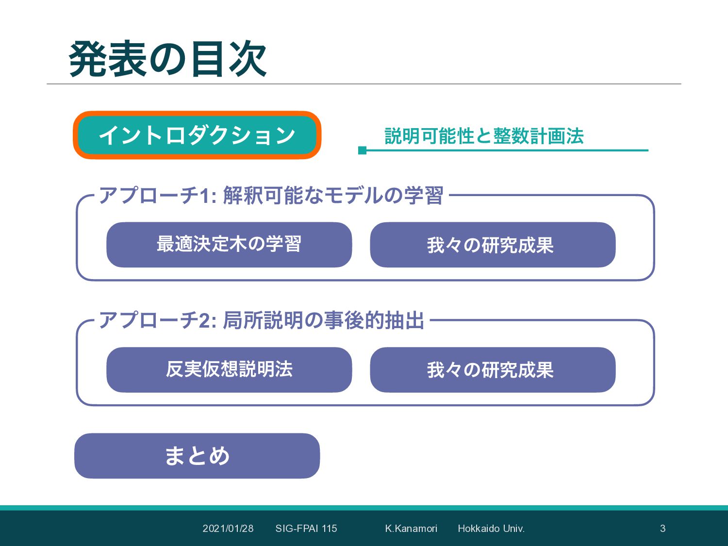
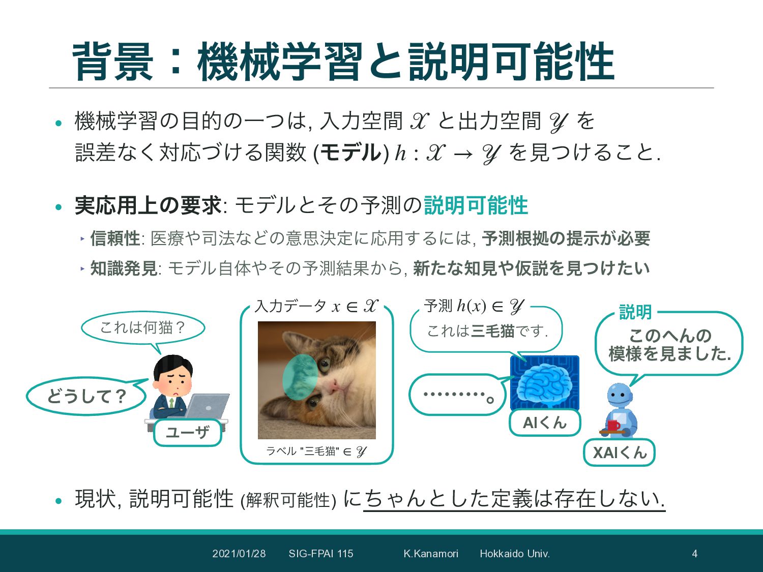
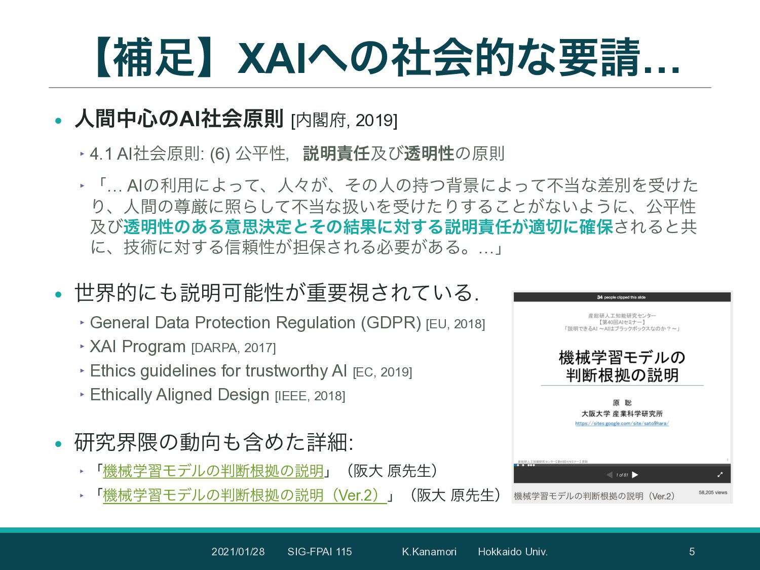
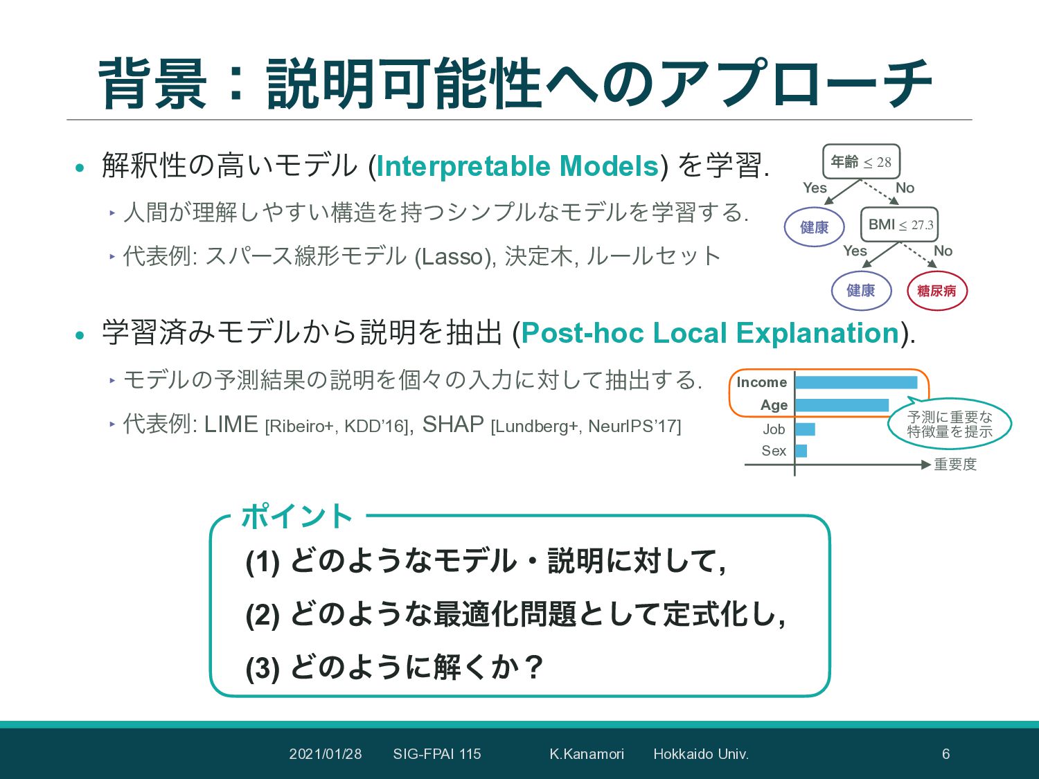
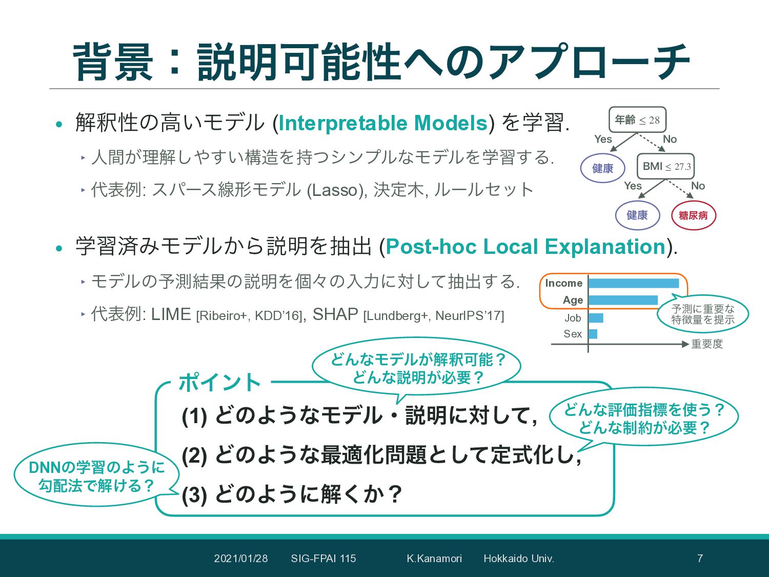
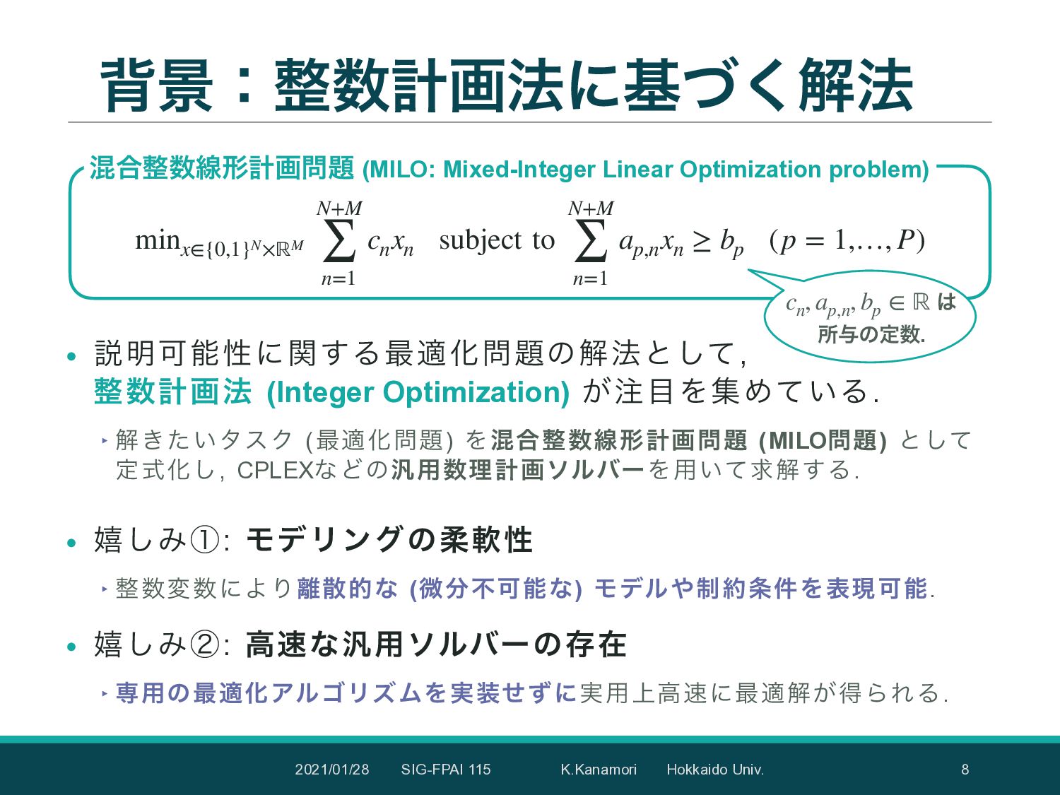
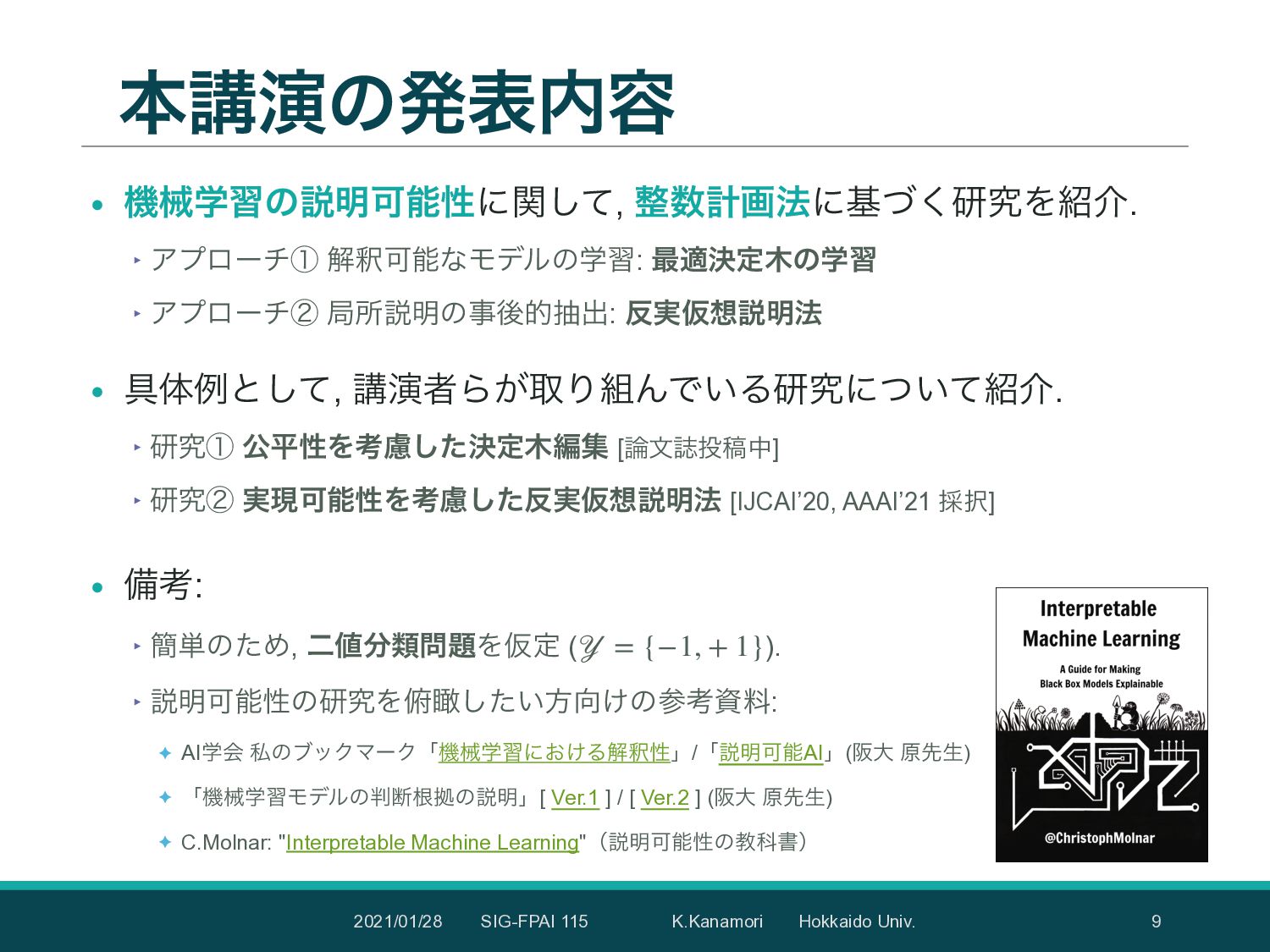
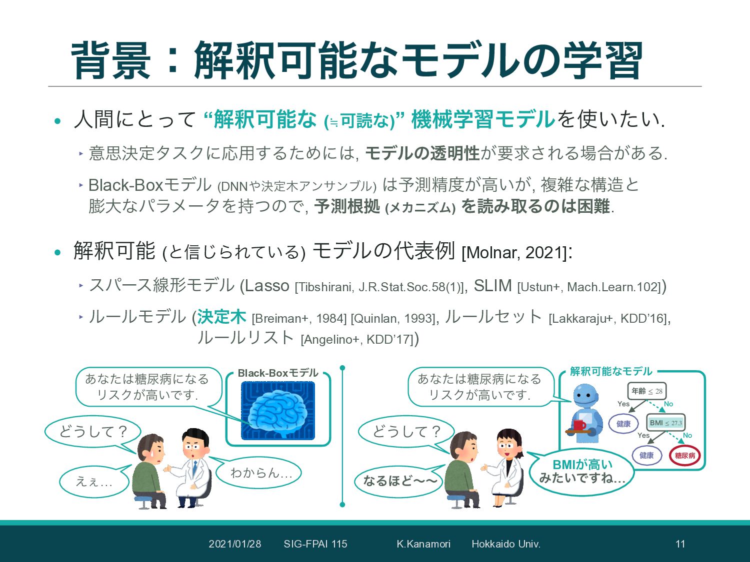
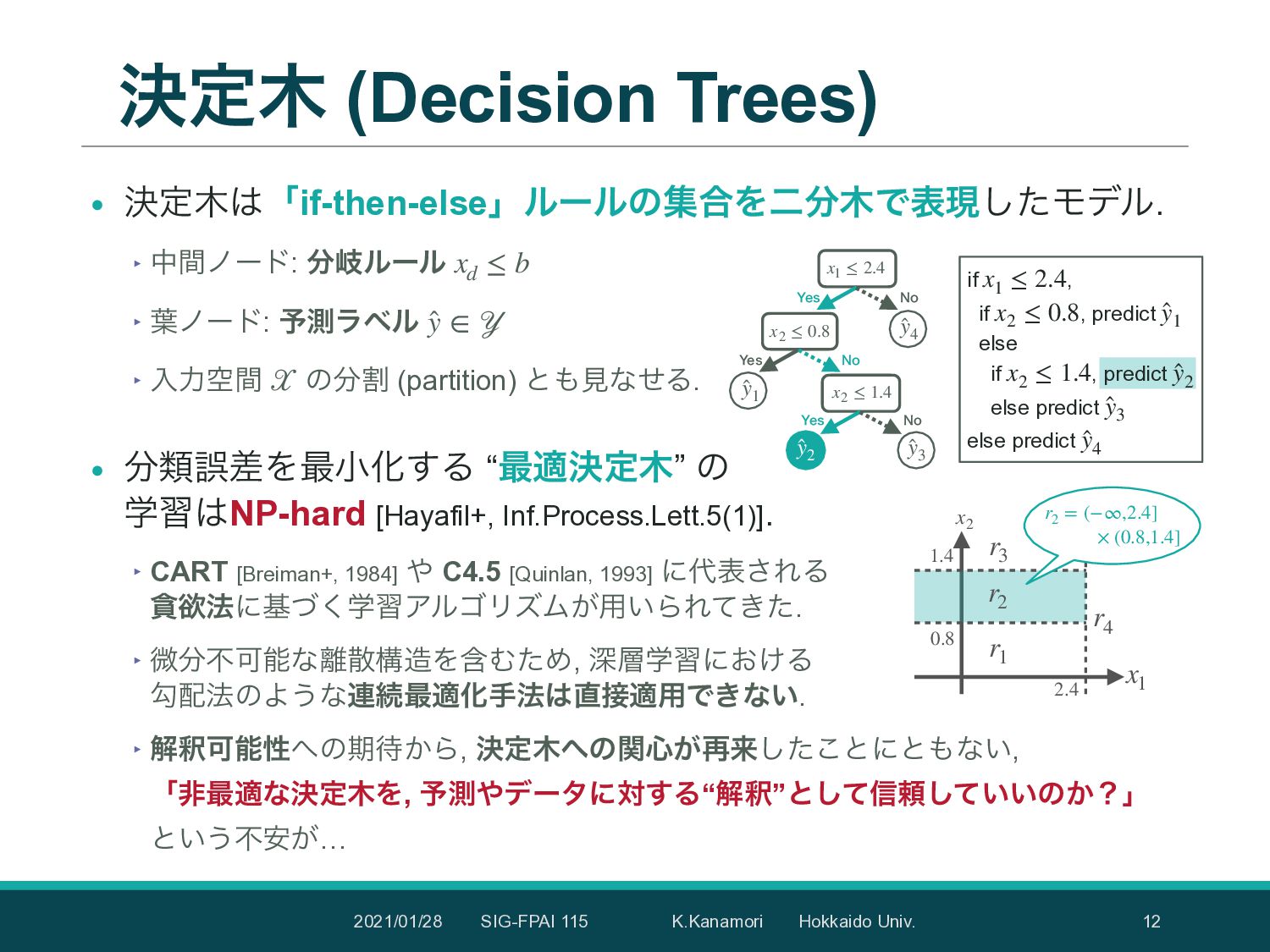
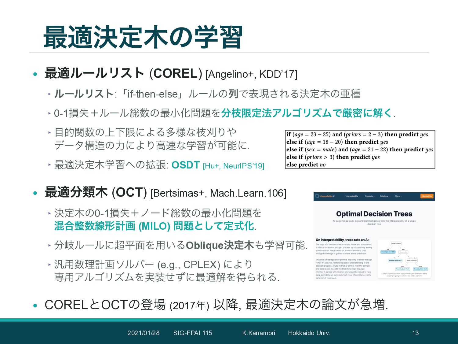
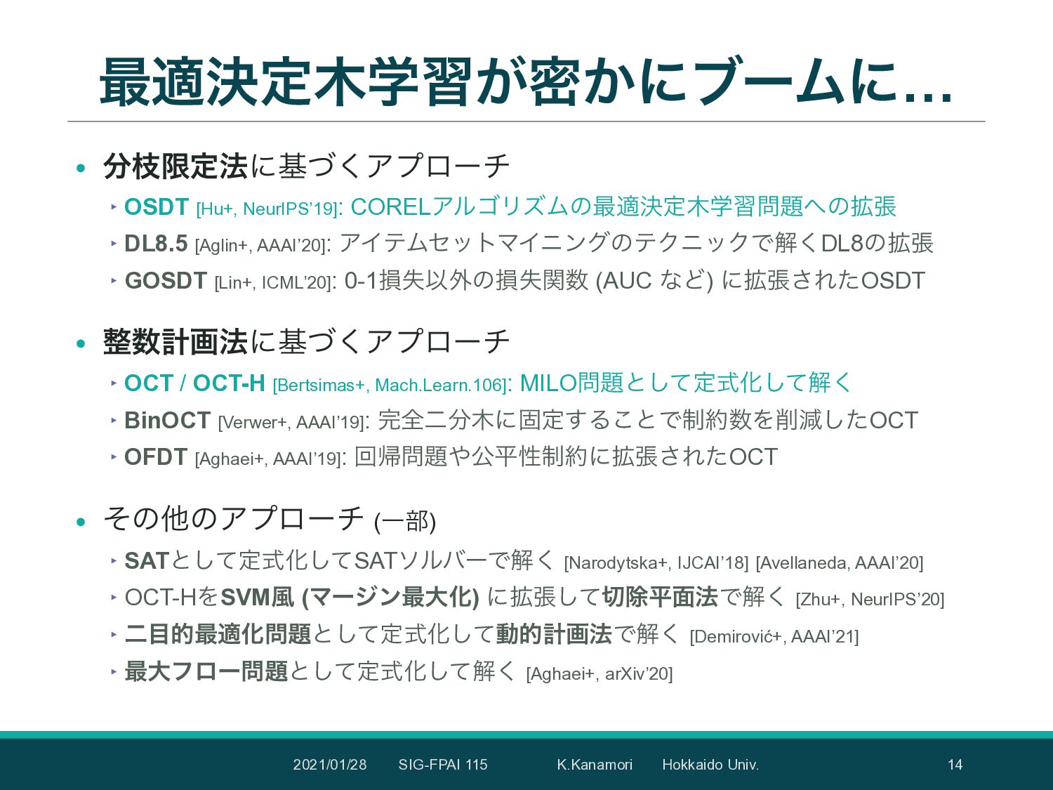
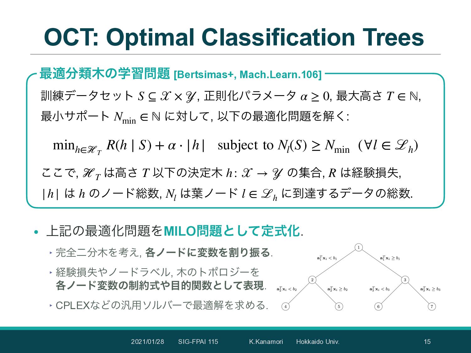
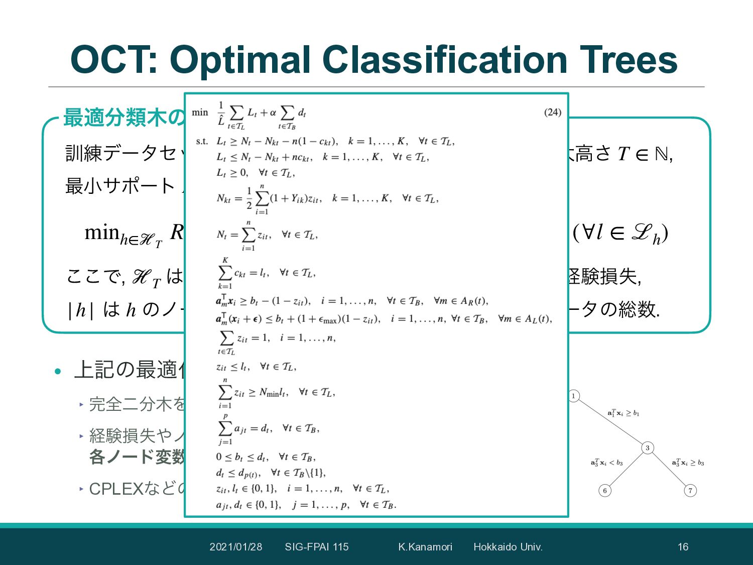
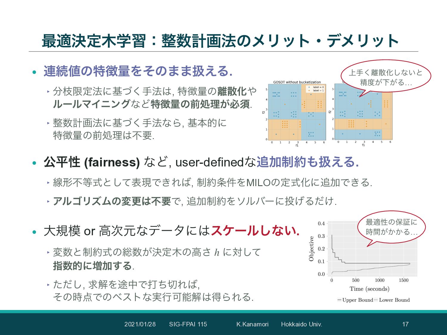
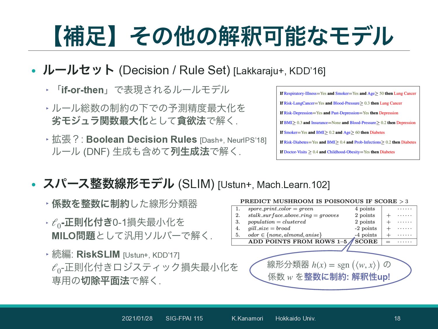
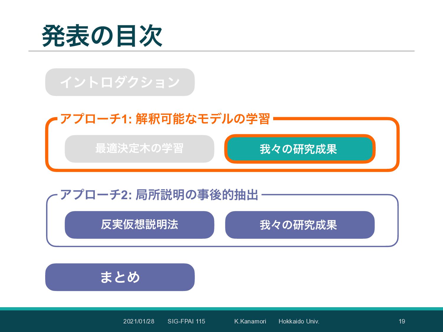
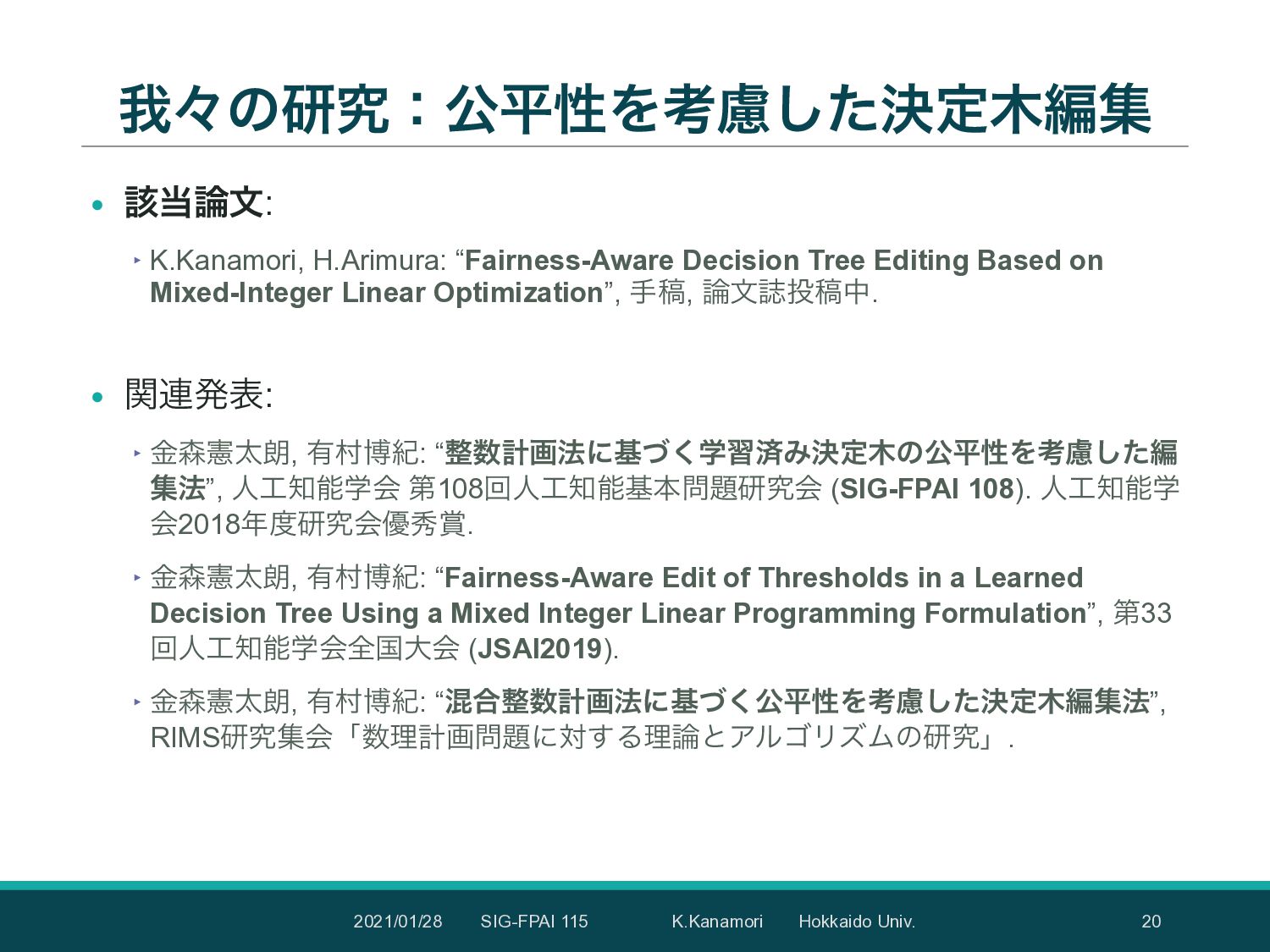
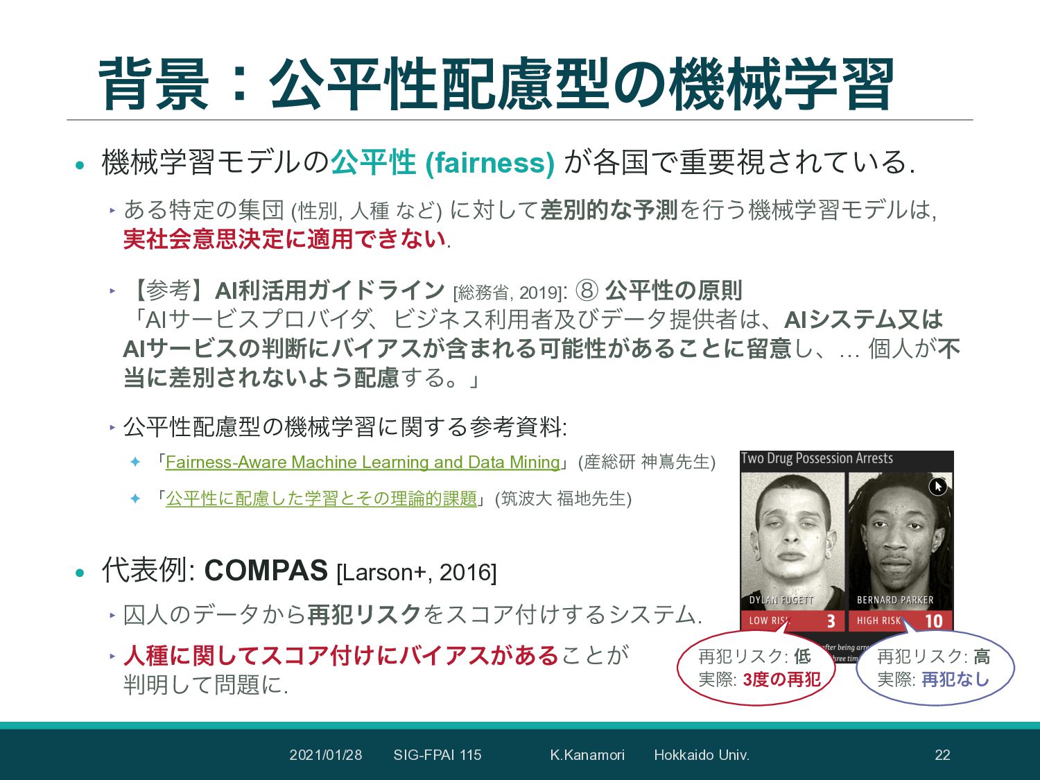
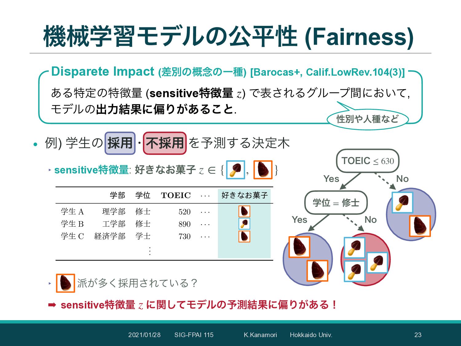
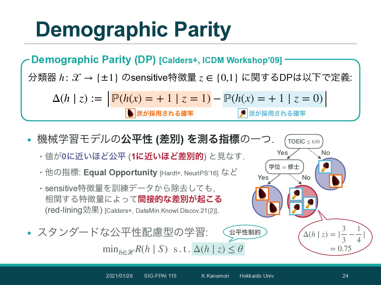
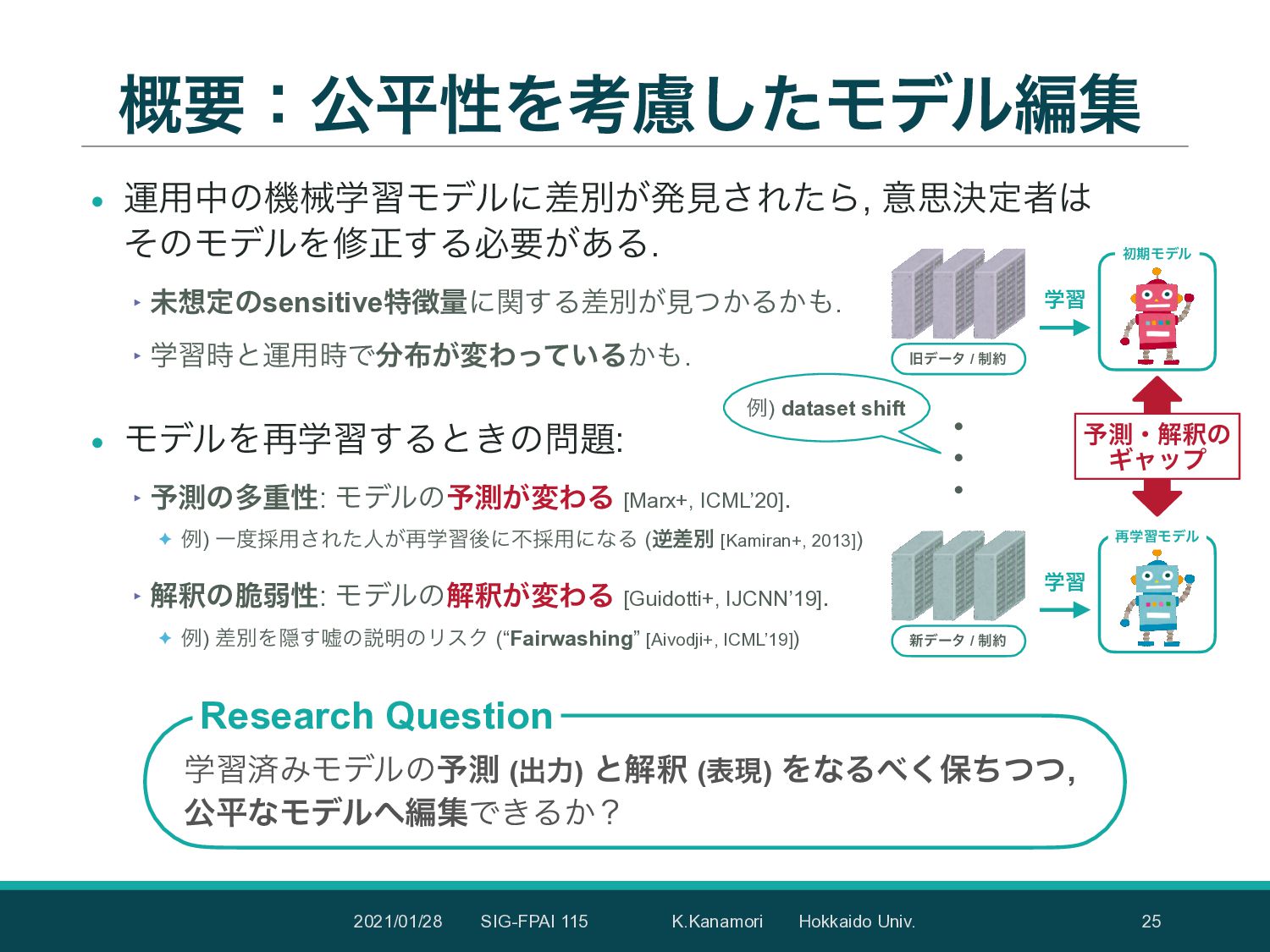
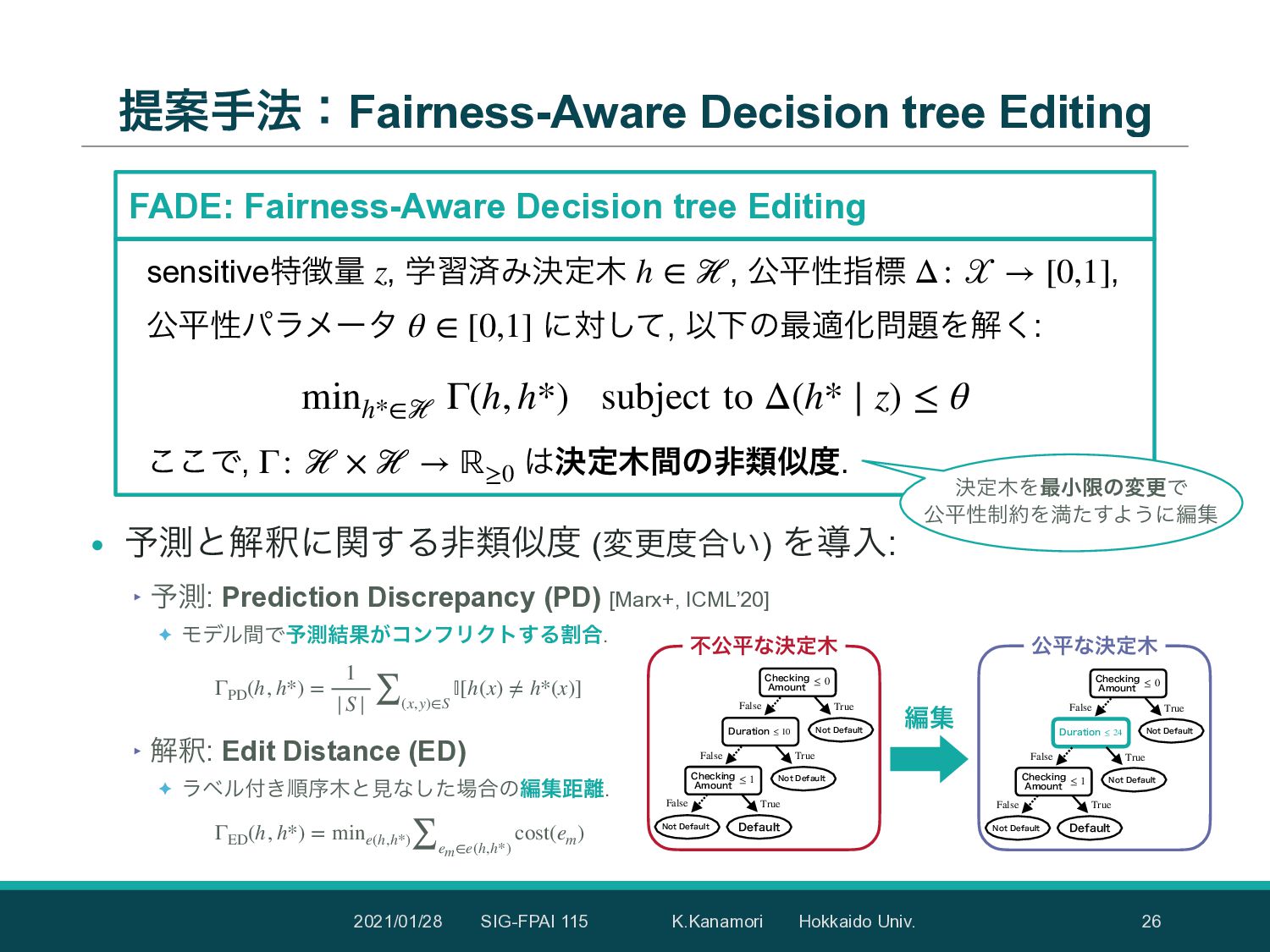
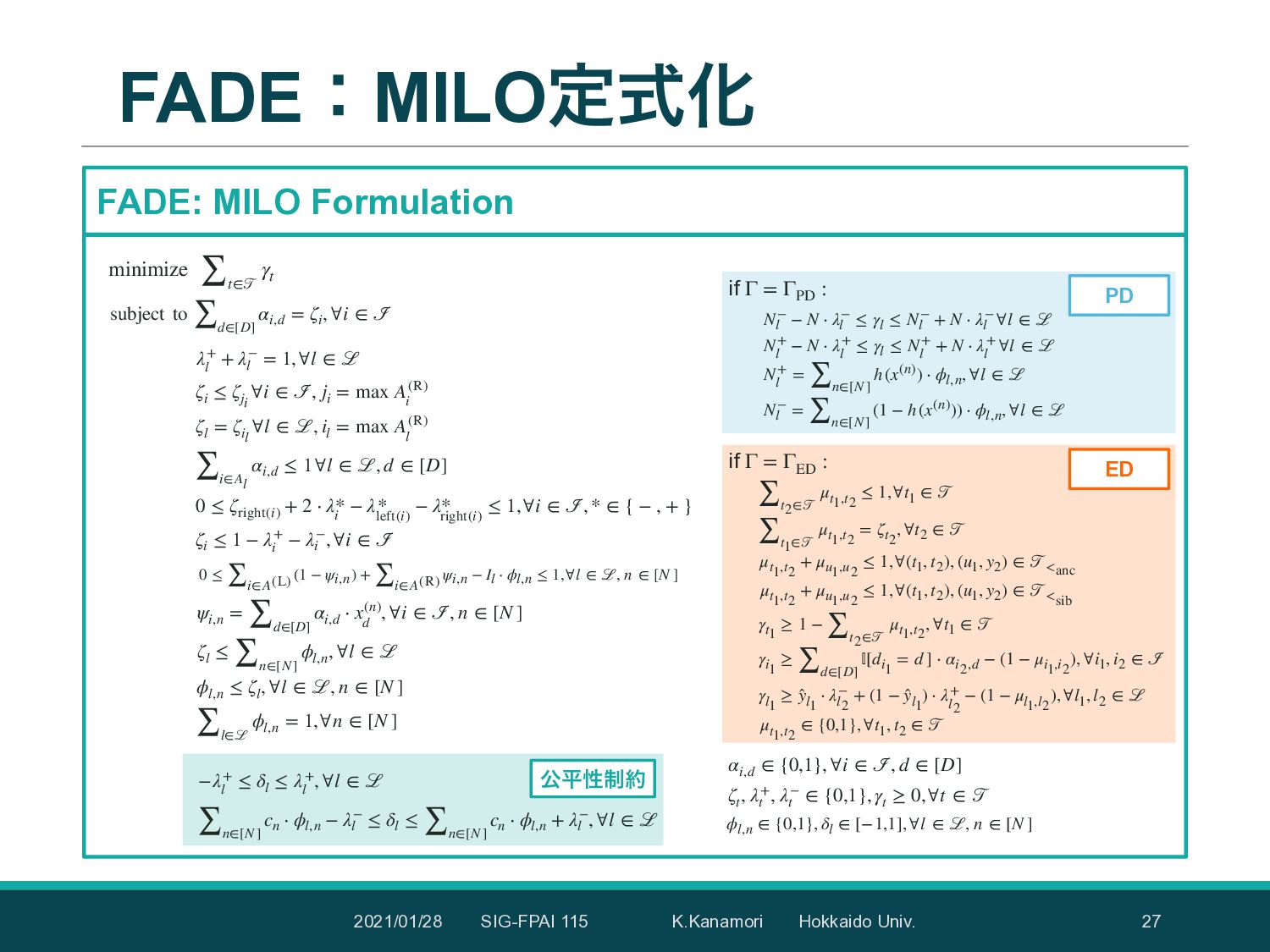
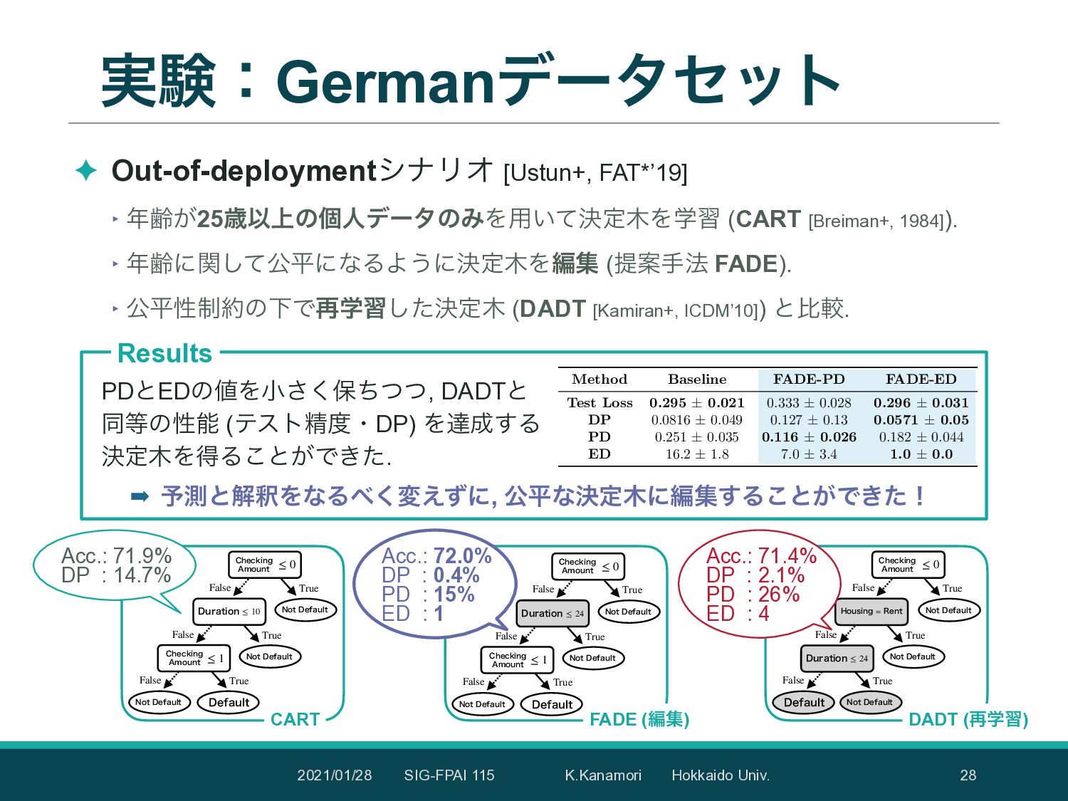
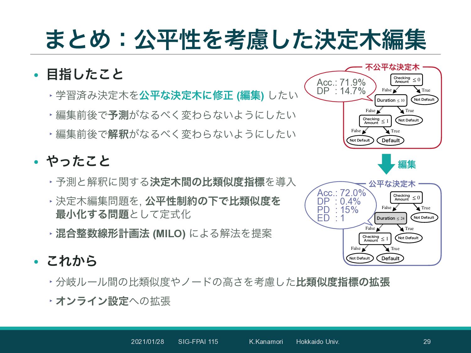
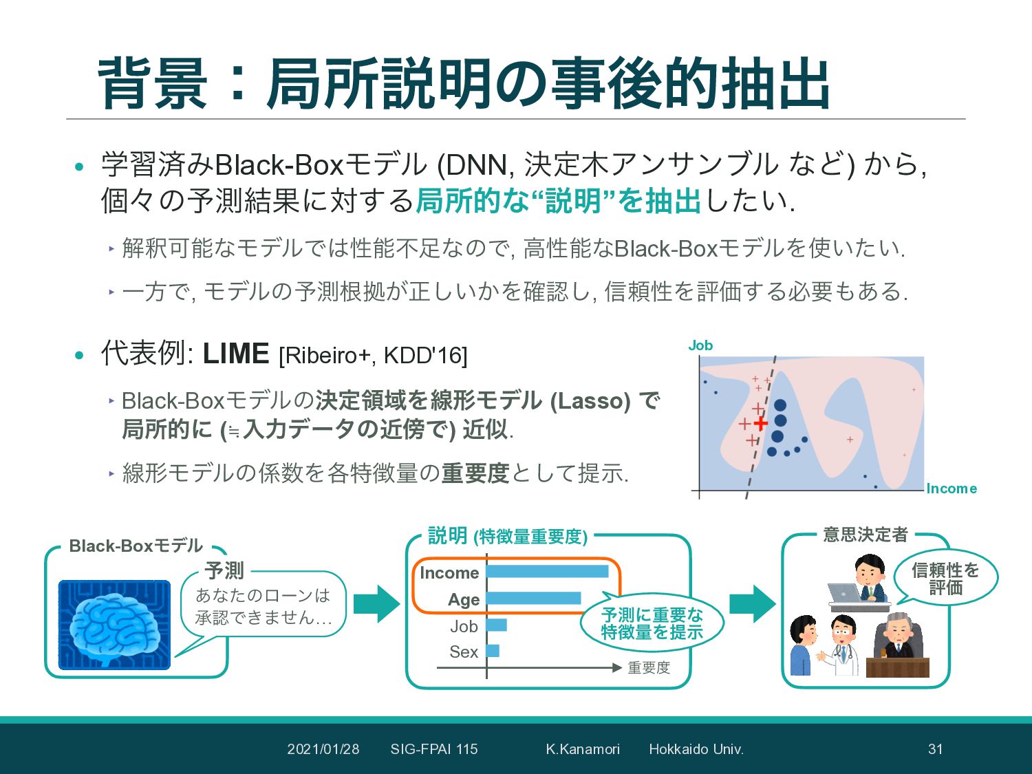
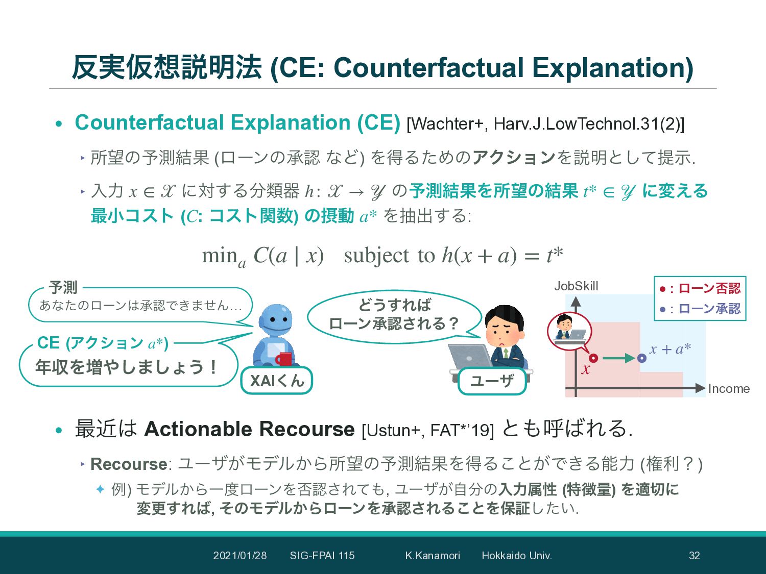
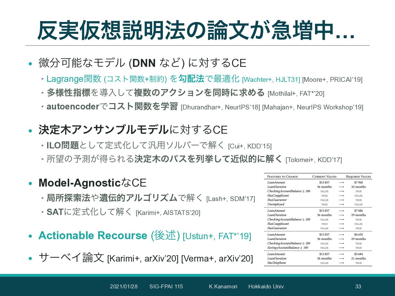
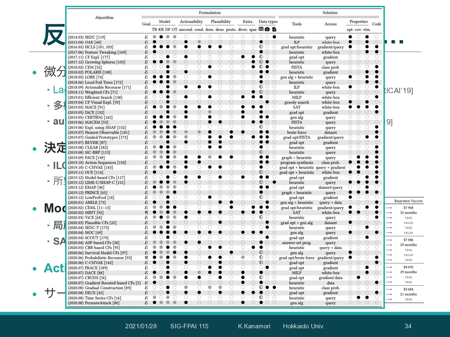
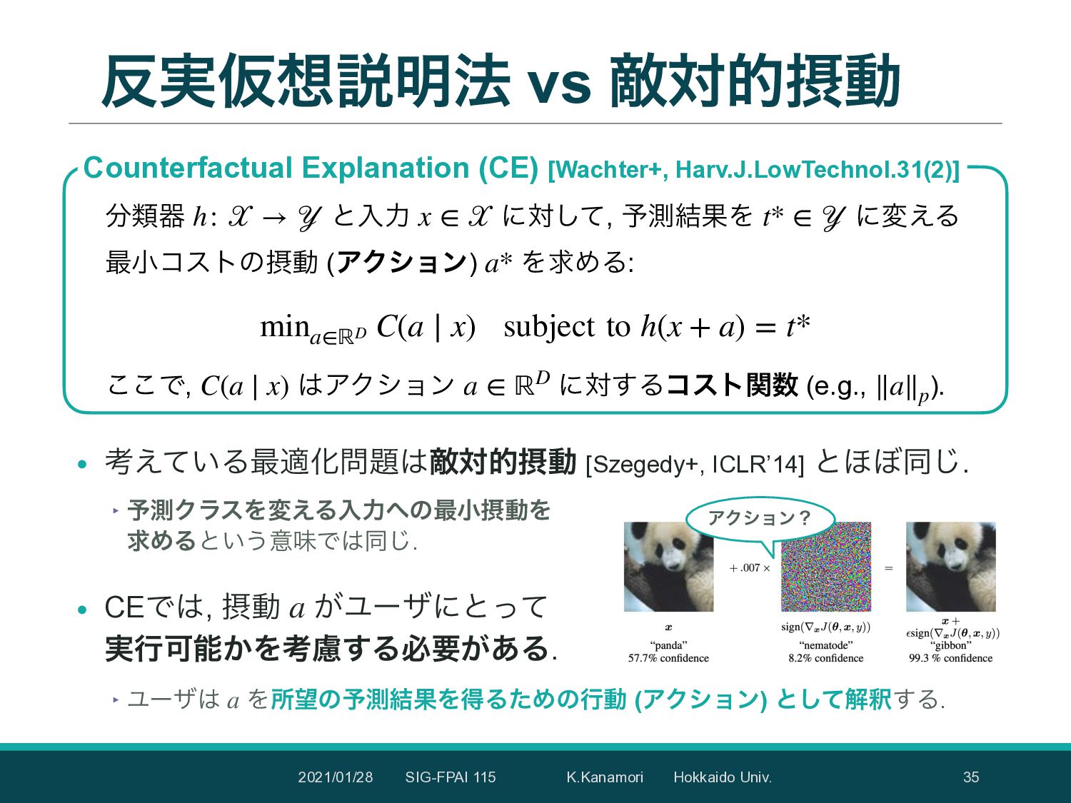
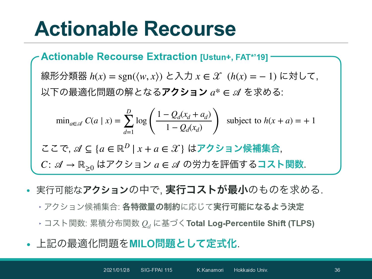
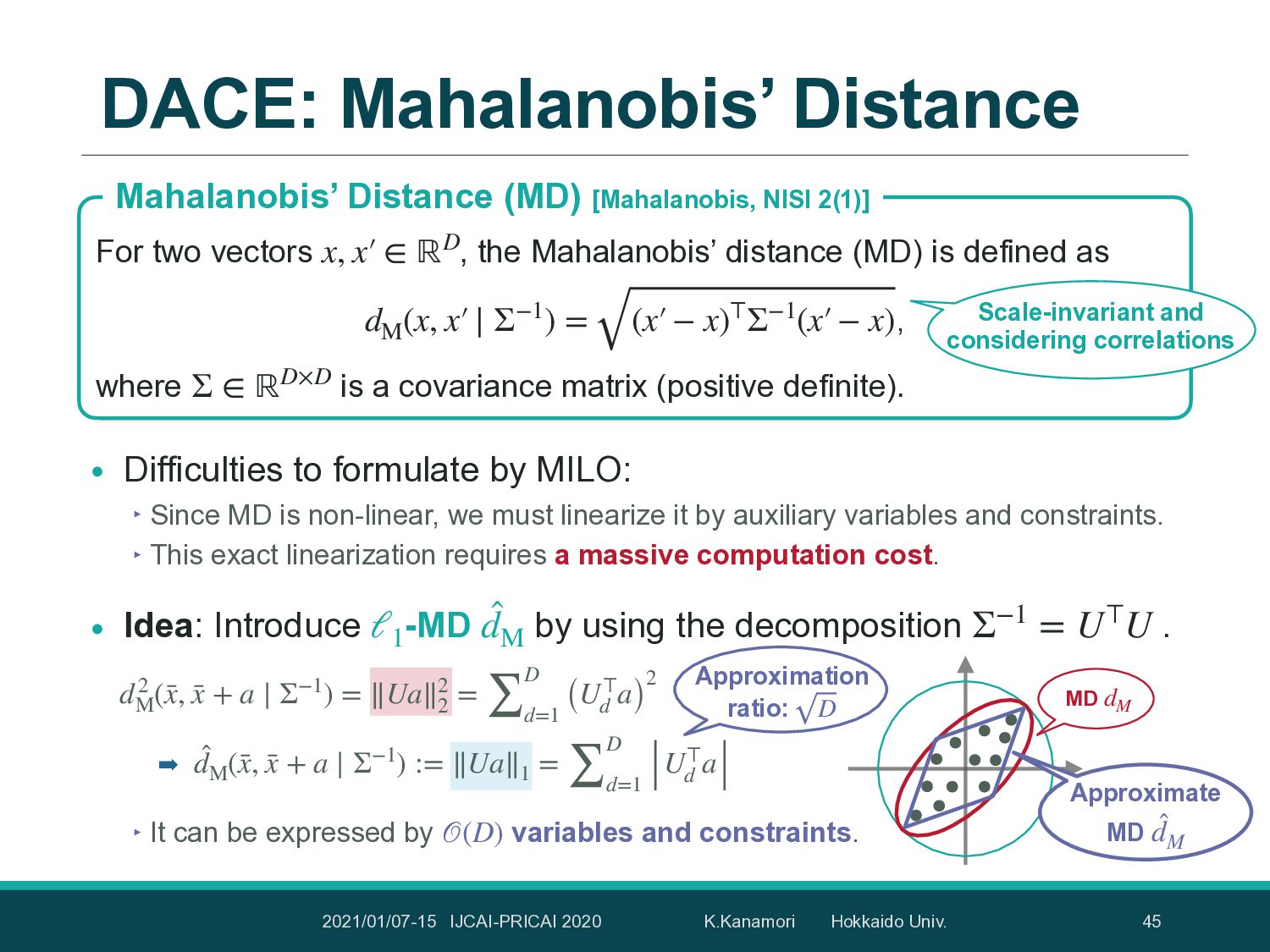
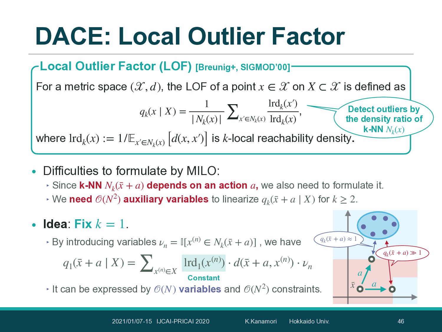
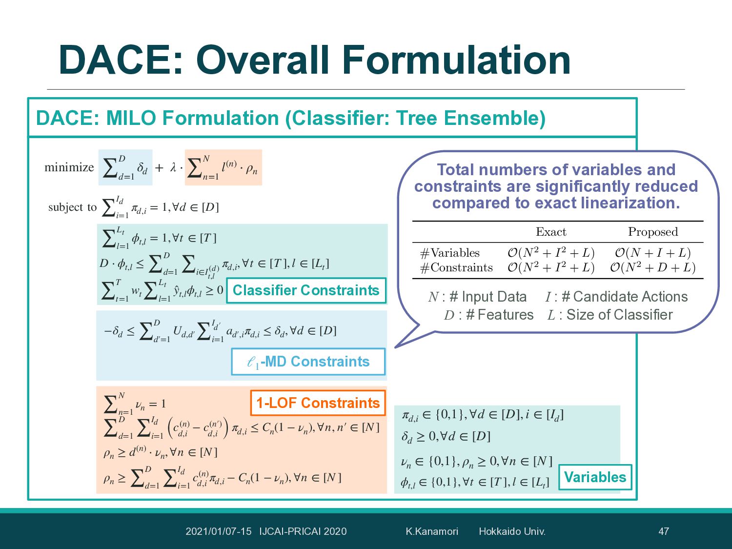
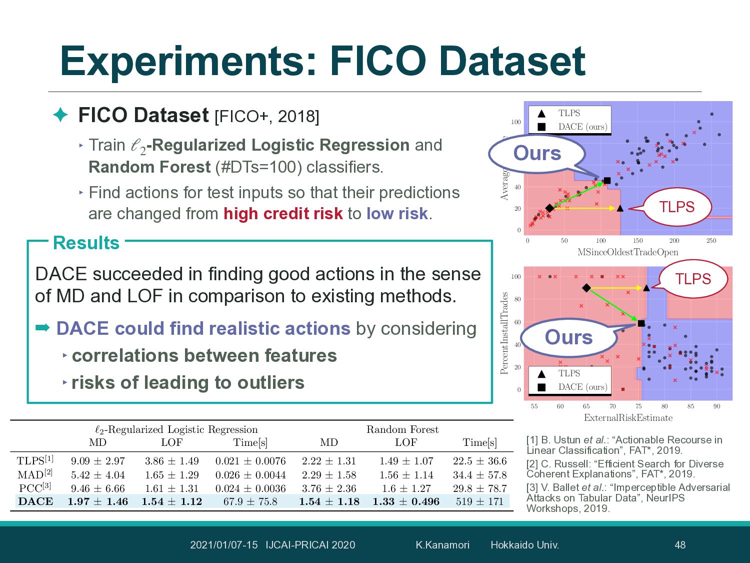
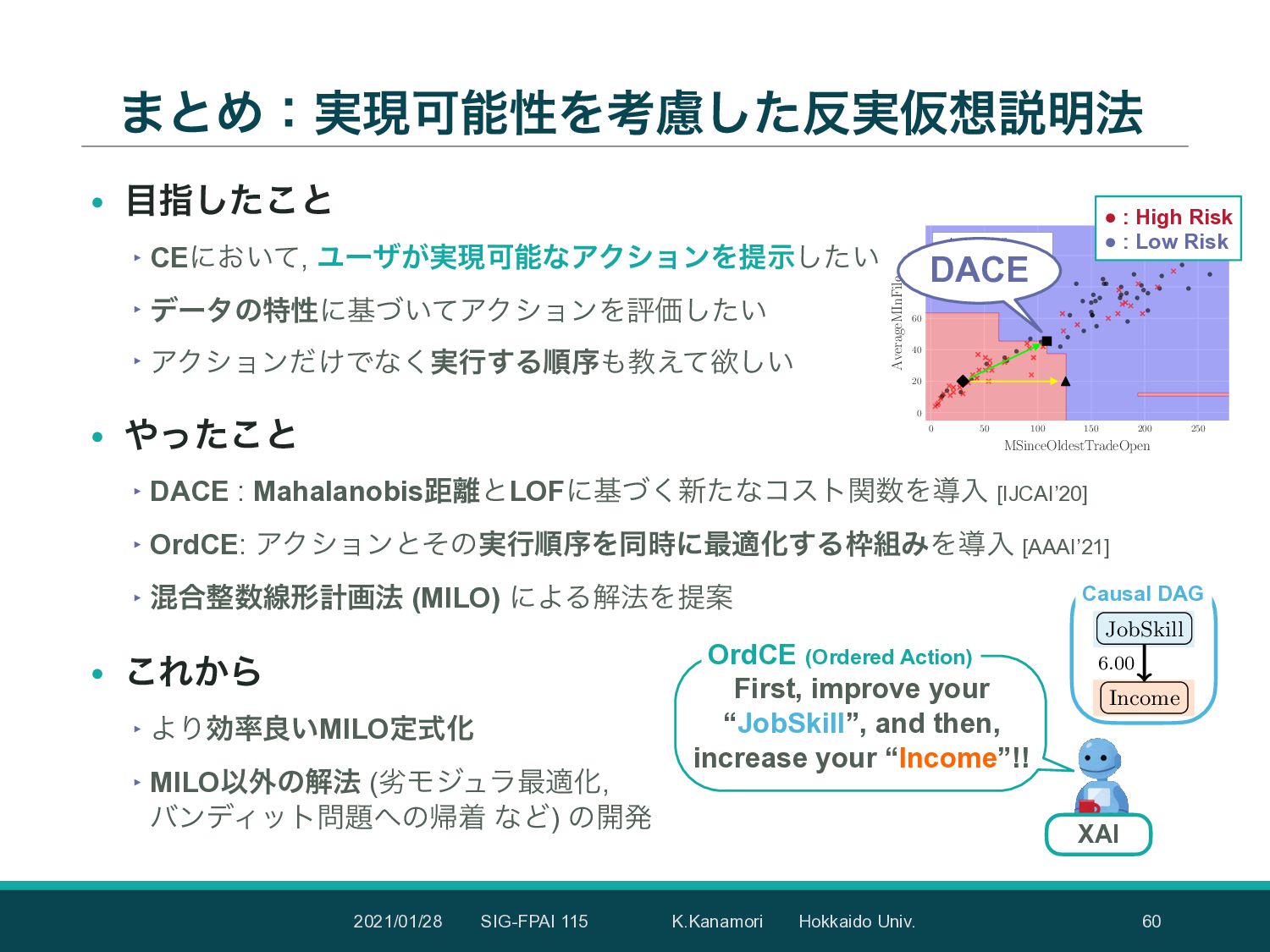
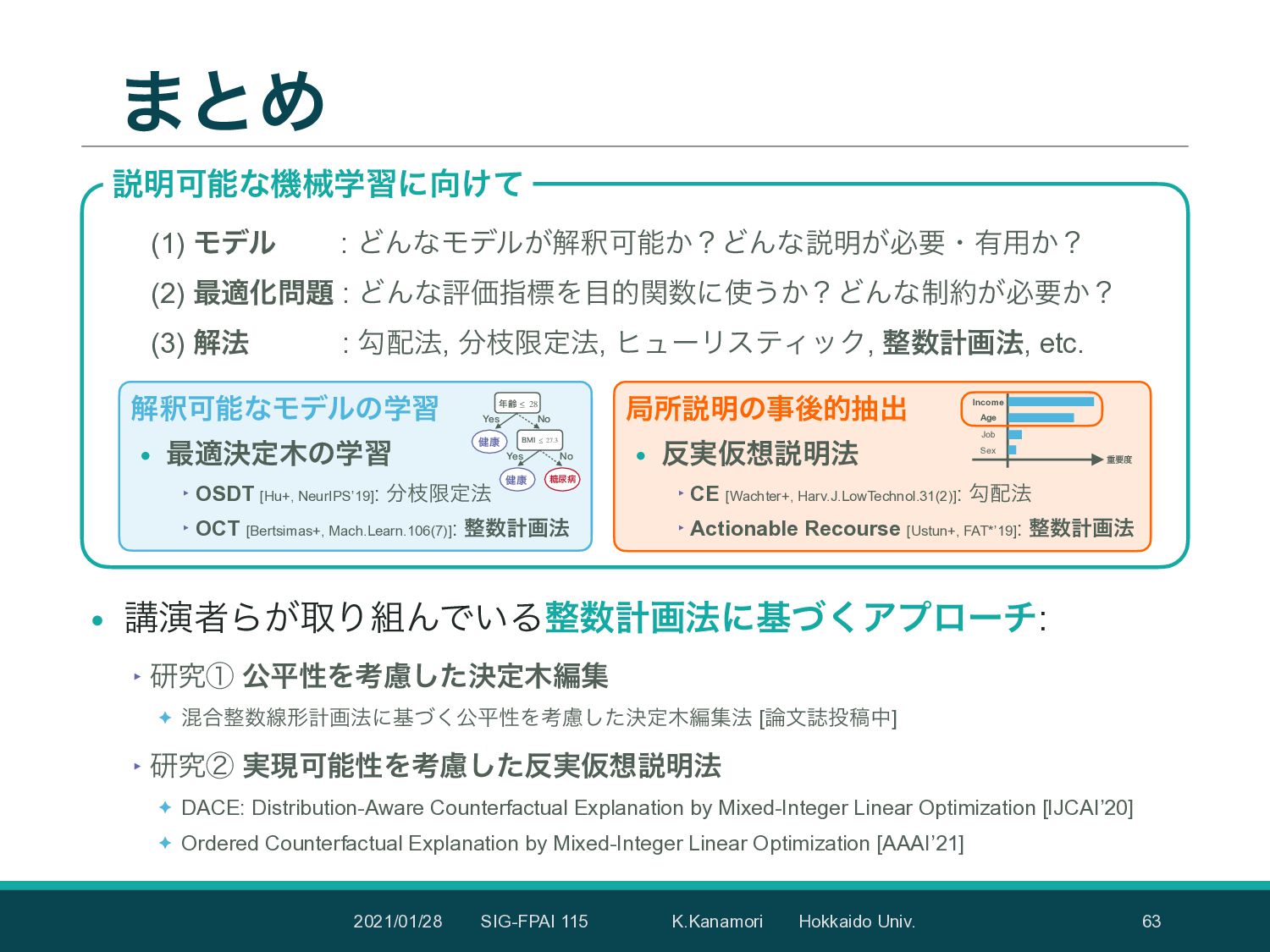
深層学習に代表される機械学習手法の発展により,機械学習モデルが医療や金融などといった実社会意思決定の現場に応用され始めている.これに伴い,機械学習モデルの予測根拠や判断基準を人間が理解可能な形で提示できる“説明可能性 (Explainability) ”の実現が重要視されており,近年活発に研究が行われている.説明可能性の実現を目的としたアプローチには,大きく分けて,(1)決定木に代表される大域的に解釈可能なモデル (Interpretable Models) を学習する方法と,(2)学習済みモデルから局所的な説明を抽出する方法 (Post-hoc Local Explanation) の2つが存在する.これらのアプローチの多くは,そのタスクを最適化問題(L0正則化つき経験損失最小化など)として定式化することで,機械学習モデルの“説明”を数理モデル化することを試みている.しかし,このような最適化問題は,離散的な性質を持つ制約条件の存在や目的関数の微分不可能性などにより,従来の機械学習で広く用いられてきた連続最適化アルゴリズムを直接適用できない場合が多い.これに対して,近年,その柔軟なモデリング能力と汎用ソルバーの発展を背景として,整数計画法 (Integer Programming) に基づく最適化手法が注目を集めている.本講演では,機械学習の説明可能性の実現を目的とした最適化問題に対する整数計画法に基づくアプローチとして,(1)最適決定木 (Optimal Decision Trees [Bertsimas+, Mach.Learn.106]) の学習と,(2)反実仮想説明法 (Counterfactual Explanation [Wachter+, Harv.J.LowTechnol.31(2)]) について紹介する.加えて,整数計画法に基づく手法の具体例として,本講演者が取り組んでいる(1)公平性を考慮した決定木編集法 [Kanamori+, Trans.on JSAI 36(4)]と,(2)実現可能性を考慮した反実仮想説明法 [Kanamori+, IJCAI'20, AAAI'21] についても紹介する.

kelicht

January 28, 2021
Tweet

More Decks by kelicht

Other Decks in Science

Transcript

  1. 2021/01/28 SIG-FPAI 115 K.Kanamori Hokkaido Univ. 1 ੔਺ܭը๏ʹجͮ͘ 
 આ໌Մೳͳػցֶश΁ͷ

    
 Ξϓϩʔν ਓ޻஌ೳֶձ ୈ115ճਓ޻஌ೳجຊ໰୊ݚڀձ SIG-FPAI 115 ۚ৿ ݑଠ࿕ ๺ւಓେֶ େֶӃ৘ใՊֶӃ ത࢜ޙظ՝ఔ1೥ [email protected] | https://sites.google.com/view/kentarokanamori
  2. 2021/01/28 SIG-FPAI 115 K.Kanamori Hokkaido Univ. 2 • ۚ৿ ݑଠ࿕

    (͔ͳ΋Γ ͚ΜͨΖ͏) ‣ ๺େ ৘ใ஌ࣝωοτϫʔΫݚڀࣨ (ࢦಋڭһ: ༗ଜതل ڭत) ‣ ത࢜ޙظ՝ఔ1೥ɾֶৼಛผݚڀһDC1 • ڵຯ͕͋Δ͜ͱ: ‣ ػցֶशͷઆ໌ՄೳੑɾղऍՄೳੑɾެฏੑ ‣ ཭ࢄ࠷దԽ (੔਺ܭը๏, ྼϞδϡϥ࠷దԽ, …) • ओͳݚڀۀ੷: ‣ “੔਺ܭը๏ʹجֶͮ͘शࡁΈܾఆ໦ͷެฏੑΛߟྀͨ͠ฤू๏”, SIG-FPAI 108, 2018೥౓ݚڀձ༏ल৆. ‣ “DACE: Distribution-Aware Counterfactual Explanation by Mixed-Integer Linear Optimization”, IJCAI 2020. ‣ “Ordered Counterfactual Explanation by Mixed-Integer Linear Optimization”, AAAI 2021 (to appear). ࣗݾ঺հ
  3. 2021/01/28 SIG-FPAI 115 K.Kanamori Hokkaido Univ. ൃදͷ໨࣍ 3 ΠϯτϩμΫγϣϯ Ξϓϩʔν1:

    ղऍՄೳͳϞσϧͷֶश ࠷దܾఆ໦ͷֶश ·ͱΊ զʑͷݚڀ੒Ռ Ξϓϩʔν2: ہॴઆ໌ͷࣄޙతநग़ ൓࣮Ծ૝આ໌๏ զʑͷݚڀ੒Ռ આ໌Մೳੑͱ੔਺ܭը๏
  4. 2021/01/28 SIG-FPAI 115 K.Kanamori Hokkaido Univ. എܠɿػցֶशͱઆ໌Մೳੑ 4 • ػցֶशͷ໨తͷҰͭ͸,

    ೖྗۭؒ ͱग़ྗۭؒ Λ 
 ޡࠩͳ͘ରԠ͚ͮΔؔ਺ (Ϟσϧ) Λݟ͚ͭΔ͜ͱ. • ࣮Ԡ༻্ͷཁٻ: Ϟσϧͱͦͷ༧ଌͷઆ໌Մೳੑ ‣ ৴པੑ: ҩྍ΍࢘๏ͳͲͷҙࢥܾఆʹԠ༻͢Δʹ͸, ༧ଌࠜڌͷఏ͕ࣔඞཁ ‣ ஌ࣝൃݟ: Ϟσϧࣗମ΍ͦͷ༧ଌ݁Ռ͔Β, ৽ͨͳ஌ݟ΍ԾઆΛݟ͚͍ͭͨ • ݱঢ়, આ໌Մೳੑ (ղऍՄೳੑ) ʹͪΌΜͱͨ͠ఆٛ͸ଘࡏ͠ͳ͍. 𝒳 𝒴 h : 𝒳 → 𝒴 Ϣʔβ AI͘Μ ೖྗσʔλ x ∈ 𝒳 ϥϕϧ "ࡾໟೣ" ∈ 𝒴 Ͳ͏ͯ͠ʁ ͜Ε͸ࡾໟೣͰ͢. ༧ଌ h(x) ∈ 𝒴 ͜Ε͸Կೣʁ ʜʜʜɻ XAI͘Μ ͜ͷ΁Μͷ 
 ໛༷Λݟ·ͨ͠. આ໌
  5. 2021/01/28 SIG-FPAI 115 K.Kanamori Hokkaido Univ. ʲิ଍ʳXAI΁ͷࣾձతͳཁ੥… 5 • ਓؒத৺ͷAIࣾձݪଇ

    [಺ֳ෎, 2019] ‣ 4.1 AIࣾձݪଇ: (6) ެฏੑɼઆ໌੹೚ٴͼಁ໌ੑͷݪଇ ‣ ʮ… AIͷར༻ʹΑͬͯɺਓʑ͕ɺͦͷਓͷ࣋ͭഎܠʹΑͬͯෆ౰ͳࠩผΛड͚ͨ ΓɺਓؒͷଚݫʹরΒͯ͠ෆ౰ͳѻ͍Λड͚ͨΓ͢Δ͜ͱ͕ͳ͍Α͏ʹɺެฏੑ ٴͼಁ໌ੑͷ͋Δҙࢥܾఆͱͦͷ݁Ռʹର͢Δઆ໌੹೚͕ద੾ʹ֬อ͞ΕΔͱڞ ʹɺٕज़ʹର͢Δ৴པੑ͕୲อ͞ΕΔඞཁ͕͋Δɻ…ʯ • ੈքతʹ΋આ໌Մೳੑ͕ॏཁࢹ͞Ε͍ͯΔ. ‣ General Data Protection Regulation (GDPR) [EU, 2018] ‣ XAI Program [DARPA, 2017] ‣ Ethics guidelines for trustworthy AI [EC, 2019] ‣ Ethically Aligned Design [IEEE, 2018] • ݚڀք۾ͷಈ޲΋ؚΊͨৄࡉ: ‣ ʮػցֶशϞσϧͷ൑அࠜڌͷઆ໌ʯʢࡕେ ݪઌੜʣ ‣ ʮػցֶशϞσϧͷ൑அࠜڌͷઆ໌ʢVer.2ʣʯʢࡕେ ݪઌੜʣ
  6. 2021/01/28 SIG-FPAI 115 K.Kanamori Hokkaido Univ. എܠɿઆ໌Մೳੑ΁ͷΞϓϩʔν 6 • ղऍੑͷߴ͍Ϟσϧ

    (Interpretable Models) Λֶश. ‣ ਓ͕ؒཧղ͠΍͍͢ߏ଄Λ࣋ͭγϯϓϧͳϞσϧΛֶश͢Δ. ‣ ୅දྫ: εύʔεઢܗϞσϧ (Lasso), ܾఆ໦, ϧʔϧηοτ • ֶशࡁΈϞσϧ͔Βઆ໌Λநग़ (Post-hoc Local Explanation). ‣ Ϟσϧͷ༧ଌ݁Ռͷઆ໌Λݸʑͷೖྗʹରͯ͠நग़͢Δ. ‣ ୅දྫ: LIME [Ribeiro+, KDD’16], SHAP [Lundberg+, NeurIPS’17] (1) ͲͷΑ͏ͳϞσϧɾઆ໌ʹରͯ͠, 
 (2) ͲͷΑ͏ͳ࠷దԽ໰୊ͱͯ͠ఆࣜԽ͠, 
 (3) ͲͷΑ͏ʹղ͔͘ʁ ϙΠϯτ Income Age Job Sex ॏཁ౓ ༧ଌʹॏཁͳ ಛ௃ྔΛఏࣔ :FT /P :FT /P ೥ྸ ≤ 28 #.* ≤ 27.3 ݈߁ ౶೘ප ݈߁
  7. 2021/01/28 SIG-FPAI 115 K.Kanamori Hokkaido Univ. എܠɿઆ໌Մೳੑ΁ͷΞϓϩʔν 7 • ղऍੑͷߴ͍Ϟσϧ

    (Interpretable Models) Λֶश. ‣ ਓ͕ؒཧղ͠΍͍͢ߏ଄Λ࣋ͭγϯϓϧͳϞσϧΛֶश͢Δ. ‣ ୅දྫ: εύʔεઢܗϞσϧ (Lasso), ܾఆ໦, ϧʔϧηοτ • ֶशࡁΈϞσϧ͔Βઆ໌Λநग़ (Post-hoc Local Explanation). ‣ Ϟσϧͷ༧ଌ݁Ռͷઆ໌Λݸʑͷೖྗʹରͯ͠நग़͢Δ. ‣ ୅දྫ: LIME [Ribeiro+, KDD’16], SHAP [Lundberg+, NeurIPS’17] (1) ͲͷΑ͏ͳϞσϧɾઆ໌ʹରͯ͠, 
 (2) ͲͷΑ͏ͳ࠷దԽ໰୊ͱͯ͠ఆࣜԽ͠, 
 (3) ͲͷΑ͏ʹղ͔͘ʁ ϙΠϯτ :FT /P :FT /P ೥ྸ ≤ 28 #.* ≤ 27.3 ݈߁ ౶೘ප ݈߁ ͲΜͳධՁࢦඪΛ࢖͏ʁ ͲΜͳ੍໿͕ඞཁʁ ͲΜͳϞσϧ͕ղऍՄೳʁ ͲΜͳઆ໌͕ඞཁʁ DNNͷֶशͷΑ͏ʹ ޯ഑๏Ͱղ͚Δʁ Income Age Job Sex ॏཁ౓ ༧ଌʹॏཁͳ ಛ௃ྔΛఏࣔ
  8. 2021/01/28 SIG-FPAI 115 K.Kanamori Hokkaido Univ. എܠɿ੔਺ܭը๏ʹجͮ͘ղ๏ 8 • આ໌Մೳੑʹؔ͢Δ࠷దԽ໰୊ͷղ๏ͱͯ͠,

    
 ੔਺ܭը๏ (Integer Optimization) ͕஫໨ΛूΊ͍ͯΔ. ‣ ղ͖͍ͨλεΫ (࠷దԽ໰୊) Λࠞ߹੔਺ઢܗܭը໰୊ (MILO໰୊) ͱͯ͠ 
 ఆࣜԽ͠, CPLEXͳͲͷ൚༻਺ཧܭըιϧόʔΛ༻͍ͯٻղ͢Δ. • خ͠Έᶃ: ϞσϦϯάͷॊೈੑ ‣ ੔਺ม਺ʹΑΓ཭ࢄతͳ (ඍ෼ෆՄೳͳ) Ϟσϧ΍੍໿৚݅ΛදݱՄೳ. • خ͠Έᶄ: ߴ଎ͳ൚༻ιϧόʔͷଘࡏ ‣ ઐ༻ͷ࠷దԽΞϧΰϦζϜΛ࣮૷ͤͣʹ࣮༻্ߴ଎ʹ࠷దղ͕ಘΒΕΔ. minx∈{0,1}N×ℝM N+M ∑ n=1 cn xn subject to N+M ∑ n=1 ap,n xn ≥ bp (p = 1,…, P) ࠞ߹੔਺ઢܗܭը໰୊ (MILO: Mixed-Integer Linear Optimization problem) ͸ 
 ॴ༩ͷఆ਺. cn , ap,n , bp ∈ ℝ
  9. 2021/01/28 SIG-FPAI 115 K.Kanamori Hokkaido Univ. ຊߨԋͷൃද಺༰ 9 • ػցֶशͷઆ໌Մೳੑʹؔͯ͠,

    ੔਺ܭը๏ʹجͮ͘ݚڀΛ঺հ. ‣ Ξϓϩʔνᶃ ղऍՄೳͳϞσϧͷֶश: ࠷దܾఆ໦ͷֶश ‣ Ξϓϩʔνᶄ ہॴઆ໌ͷࣄޙతநग़: ൓࣮Ծ૝આ໌๏ • ۩ମྫͱͯ͠, ߨԋऀΒ͕औΓ૊ΜͰ͍Δݚڀʹ͍ͭͯ঺հ. ‣ ݚڀᶃ ެฏੑΛߟྀܾͨ͠ఆ໦ฤू [࿦จࢽ౤ߘத] ‣ ݚڀᶄ ࣮ݱՄೳੑΛߟྀͨ͠൓࣮Ծ૝આ໌๏ [IJCAI’20, AAAI’21 ࠾୒] • උߟ: ‣ ؆୯ͷͨΊ, ೋ஋෼ྨ໰୊ΛԾఆ ( ). ‣ આ໌ՄೳੑͷݚڀΛ၆ᛌ͍ͨ͠ํ޲͚ͷࢀߟࢿྉ: ✦ AIֶձ ࢲͷϒοΫϚʔΫʮػցֶशʹ͓͚Δղऍੑʯ/ʮઆ໌ՄೳAIʯ(ࡕେ ݪઌੜ) ✦ ʮػցֶशϞσϧͷ൑அࠜڌͷઆ໌ʯ[ Ver.1 ] / [ Ver.2 ] (ࡕେ ݪઌੜ) ✦ C.Molnar: "Interpretable Machine Learning"ʢઆ໌ՄೳੑͷڭՊॻʣ 𝒴 = {−1, + 1}
  10. 2021/01/28 SIG-FPAI 115 K.Kanamori Hokkaido Univ. ൃදͷ໨࣍ 10 Ξϓϩʔν1: ղऍՄೳͳϞσϧͷֶश

    ࠷దܾఆ໦ͷֶश զʑͷݚڀ੒Ռ Ξϓϩʔν2: ہॴઆ໌ͷࣄޙతநग़ ൓࣮Ծ૝આ໌๏ զʑͷݚڀ੒Ռ ΠϯτϩμΫγϣϯ ·ͱΊ
  11. 2021/01/28 SIG-FPAI 115 K.Kanamori Hokkaido Univ. എܠɿղऍՄೳͳϞσϧͷֶश 11 • ਓؒʹͱͬͯ

    “ղऍՄೳͳ (≒Մಡͳ)” ػցֶशϞσϧΛ࢖͍͍ͨ. ‣ ҙࢥܾఆλεΫʹԠ༻͢ΔͨΊʹ͸, Ϟσϧͷಁ໌ੑ͕ཁٻ͞ΕΔ৔߹͕͋Δ. ‣ Black-BoxϞσϧ (DNN΍ܾఆ໦Ξϯαϯϒϧ) ͸༧ଌਫ਼౓͕ߴ͍͕, ෳࡶͳߏ଄ͱ 
 ๲େͳύϥϝʔλΛ࣋ͭͷͰ, ༧ଌࠜڌ (ϝΧχζϜ) ΛಡΈऔΔͷ͸ࠔ೉. • ղऍՄೳ (ͱ৴͡ΒΕ͍ͯΔ) Ϟσϧͷ୅දྫ [Molnar, 2021]: ‣ εύʔεઢܗϞσϧ (Lasso [Tibshirani, J.R.Stat.Soc.58(1)], SLIM [Ustun+, Mach.Learn.102]) ‣ ϧʔϧϞσϧ (ܾఆ໦ [Breiman+, 1984] [Quinlan, 1993], ϧʔϧηοτ [Lakkaraju+, KDD’16], 
 ϧʔϧϦετ [Angelino+, KDD’17]) Black-BoxϞσϧ ͋ͳͨ͸౶೘පʹͳΔ 
 ϦεΫ͕ߴ͍Ͱ͢. Ͳ͏ͯ͠ʁ ͑͐… Θ͔ΒΜ… :FT /P :FT /P ೥ྸ ≤ 28 #.* ≤ 27.3 ݈߁ ౶೘ප ݈߁ ղऍՄೳͳϞσϧ Ͳ͏ͯ͠ʁ ͳΔ΄Ͳʙʙ BMI͕ߴ͍ 
 Έ͍ͨͰ͢Ͷ… ͋ͳͨ͸౶೘පʹͳΔ 
 ϦεΫ͕ߴ͍Ͱ͢.
  12. 2021/01/28 SIG-FPAI 115 K.Kanamori Hokkaido Univ. ܾఆ໦ (Decision Trees) 12

    • ܾఆ໦͸ʮif-then-elseʯϧʔϧͷू߹Λೋ෼໦Ͱදݱͨ͠Ϟσϧ. ‣ தؒϊʔυ: ෼ذϧʔϧ ‣ ༿ϊʔυ: ༧ଌϥϕϧ ‣ ೖྗۭؒ ͷ෼ׂ (partition) ͱ΋ݟͳͤΔ. • ෼ྨޡࠩΛ࠷খԽ͢Δ “࠷దܾఆ໦” ͷ 
 ֶश͸NP-hard [Hayafil+, Inf.Process.Lett.5(1)]. ‣ CART [Breiman+, 1984] ΍ C4.5 [Quinlan, 1993] ʹ୅ද͞ΕΔ 
 ᩦཉ๏ʹجֶͮ͘शΞϧΰϦζϜ͕༻͍ΒΕ͖ͯͨ. ‣ ඍ෼ෆՄೳͳ཭ࢄߏ଄ΛؚΉͨΊ, ਂ૚ֶशʹ͓͚Δ 
 ޯ഑๏ͷΑ͏ͳ࿈ଓ࠷దԽख๏͸௚઀ద༻Ͱ͖ͳ͍. ‣ ղऍՄೳੑ΁ͷظ଴͔Β, ܾఆ໦΁ͷؔ৺͕࠶དྷͨ͜͠ͱʹͱ΋ͳ͍, 
 ʮඇ࠷దͳܾఆ໦Λ, ༧ଌ΍σʔλʹର͢Δ“ղऍ”ͱͯ͠৴པ͍͍ͯ͠ͷ͔ʁʯ 
 ͱ͍͏ෆ͕҆… xd ≤ b ̂ y ∈ 𝒴 𝒳 x1 x2 1.4 0.8 2.4 r2 r1 r3 r4 r2 = (−∞,2.4] × (0.8,1.4] x2 ≤ 0.8 x1 ≤ 2.4 x2 ≤ 1.4 :FT /P :FT /P :FT /P ̂ y2 ̂ y1 ̂ y3 ̂ y4 if , if , predict else if , predict else predict else predict x1 ≤ 2.4 x2 ≤ 0.8 ̂ y1 x2 ≤ 1.4 ̂ y2 ̂ y3 ̂ y4
  13. 2021/01/28 SIG-FPAI 115 K.Kanamori Hokkaido Univ. ࠷దܾఆ໦ͷֶश 13 • ࠷దϧʔϧϦετ

    (COREL) [Angelino+, KDD’17] ‣ ϧʔϧϦετ:ʮif-then-elseʯϧʔϧͷྻͰදݱ͞ΕΔܾఆ໦ͷѥछ ‣ 0-1ଛࣦʴϧʔϧ૯਺ͷ࠷খԽ໰୊Λ෼ࢬݶఆ๏ΞϧΰϦζϜͰݫີʹղ͘. ‣ ໨తؔ਺ͷ্ԼݶʹΑΔଟ༷ͳࢬמΓ΍ 
 σʔλߏ଄ͷྗʹΑΓߴ଎ͳֶश͕Մೳʹ. ‣ ࠷దܾఆ໦ֶश΁ͷ֦ு: OSDT [Hu+, NeurIPS’19] • ࠷ద෼ྨ໦ (OCT) [Bertsimas+, Mach.Learn.106] ‣ ܾఆ໦ͷ0-1ଛࣦʴϊʔυ૯਺ͷ࠷খԽ໰୊Λ 
 ࠞ߹੔਺ઢܗܭը (MILO) ໰୊ͱͯ͠ఆࣜԽ. ‣ ෼ذϧʔϧʹ௒ฏ໘Λ༻͍ΔObliqueܾఆ໦΋ֶशՄೳ. ‣ ൚༻਺ཧܭըιϧόʔ (e.g., CPLEX) ʹΑΓ 
 ઐ༻ΞϧΰϦζϜΛ࣮૷ͤͣʹ࠷దղΛಘΒΕΔ. • CORELͱOCTͷొ৔ (2017೥) Ҏ߱, ࠷దܾఆ໦ͷ࿦จ͕ٸ૿.
  14. 2021/01/28 SIG-FPAI 115 K.Kanamori Hokkaido Univ. ࠷దܾఆ໦ֶश͕ີ͔ʹϒʔϜʹ… 14 • ෼ࢬݶఆ๏ʹجͮ͘Ξϓϩʔν

    ‣ OSDT [Hu+, NeurIPS’19]: CORELΞϧΰϦζϜͷ࠷దܾఆ໦ֶश໰୊΁ͷ֦ு ‣ DL8.5 [Aglin+, AAAI’20]: ΞΠςϜηοτϚΠχϯάͷςΫχοΫͰղ͘DL8ͷ֦ு ‣ GOSDT [Lin+, ICML’20]: 0-1ଛࣦҎ֎ͷଛࣦؔ਺ (AUC ͳͲ) ʹ֦ு͞ΕͨOSDT • ੔਺ܭը๏ʹجͮ͘Ξϓϩʔν ‣ OCT / OCT-H [Bertsimas+, Mach.Learn.106]: MILO໰୊ͱͯ͠ఆࣜԽͯ͠ղ͘ ‣ BinOCT [Verwer+, AAAI’19]: ׬શೋ෼໦ʹݻఆ͢Δ͜ͱͰ੍໿਺Λ࡟ݮͨ͠OCT ‣ OFDT [Aghaei+, AAAI’19]: ճؼ໰୊΍ެฏੑ੍໿ʹ֦ு͞ΕͨOCT • ͦͷଞͷΞϓϩʔν (Ұ෦) ‣ SATͱͯ͠ఆࣜԽͯ͠SATιϧόʔͰղ͘ [Narodytska+, IJCAI’18] [Avellaneda, AAAI’20] ‣ OCT-HΛSVM෩ (Ϛʔδϯ࠷େԽ) ʹ֦ுͯ͠੾আฏ໘๏Ͱղ͘ [Zhu+, NeurIPS’20] ‣ ೋ໨త࠷దԽ໰୊ͱͯ͠ఆࣜԽͯ͠ಈతܭը๏Ͱղ͘ [Demirović+, AAAI’21] ‣ ࠷େϑϩʔ໰୊ͱͯ͠ఆࣜԽͯ͠ղ͘ [Aghaei+, arXiv’20]
  15. 2021/01/28 SIG-FPAI 115 K.Kanamori Hokkaido Univ. • ্هͷ࠷దԽ໰୊ΛMILO໰୊ͱͯ͠ఆࣜԽ. ‣ ׬શೋ෼໦Λߟ͑,

    ֤ϊʔυʹม਺ΛׂΓৼΔ. ‣ ܦݧଛࣦ΍ϊʔυϥϕϧ, ໦ͷτϙϩδʔΛ 
 ֤ϊʔυม਺ͷ੍໿ࣜ΍໨తؔ਺ͱͯ͠දݱ. ‣ CPLEXͳͲͷ൚༻ιϧόʔͰ࠷దղΛٻΊΔ. OCT: Optimal Classification Trees 15 ࠷ద෼ྨ໦ͷֶश໰୊ [Bertsimas+, Mach.Learn.106] ܇࿅σʔληοτ , ਖ਼ଇԽύϥϝʔλ , ࠷େߴ͞ , 
 ࠷খαϙʔτ ʹରͯ͠, ҎԼͷ࠷దԽ໰୊Λղ͘: ͜͜Ͱ, ͸ߴ͞ ҎԼͷܾఆ໦ ͷू߹, ͸ܦݧଛࣦ, 
 ͸ ͷϊʔυ૯਺, ͸༿ϊʔυ ʹ౸ୡ͢Δσʔλͷ૯਺. S ⊆ 𝒳 × 𝒴 α ≥ 0 T ∈ ℕ Nmin ∈ ℕ minh∈ℋT R(h ∣ S) + α ⋅ |h| subject to Nl (S) ≥ Nmin (∀l ∈ ℒh ) ℋT T h: 𝒳 → 𝒴 R |h| h Nl l ∈ ℒh
  16. 2021/01/28 SIG-FPAI 115 K.Kanamori Hokkaido Univ. • ্هͷ࠷దԽ໰୊ΛMILO໰୊ͱͯ͠ఆࣜԽ. ‣ ׬શೋ෼໦Λߟ͑,

    ֤ϊʔυʹม਺ΛׂΓৼΔ. ‣ ܦݧଛࣦ΍ϊʔυϥϕϧ, ໦ͷτϙϩδʔΛ 
 ֤ϊʔυม਺ͷ੍໿ࣜ΍໨తؔ਺ͱͯ͠දݱ. ‣ CPLEXͳͲͷ൚༻ιϧόʔͰ࠷దղΛٻΊΔ. OCT: Optimal Classification Trees 16 ࠷ద෼ྨ໦ͷֶश໰୊ [Bertsimas+, Mach.Learn.106] ܇࿅σʔληοτ , ਖ਼ଇԽύϥϝʔλ , ࠷େߴ͞ , 
 ࠷খαϙʔτ ʹରͯ͠, ҎԼͷ࠷దԽ໰୊Λղ͘: ͜͜Ͱ, ͸ߴ͞ ҎԼͷܾఆ໦ ͷू߹, ͸ܦݧଛࣦ, 
 ͸ ͷϊʔυ૯਺, ͸༿ϊʔυ ʹ౸ୡ͢Δσʔλͷ૯਺. S ⊆ 𝒳 × 𝒴 α ≥ 0 T ∈ ℕ Nmin ∈ ℕ minh∈ℋT R(h ∣ S) + α ⋅ |h| subject to Nl (S) ≥ Nmin (∀l ∈ ℒh ) ℋT T h: 𝒳 → 𝒴 R |h| h Nl l ∈ ℒh
  17. 2021/01/28 SIG-FPAI 115 K.Kanamori Hokkaido Univ. ࠷దܾఆ໦ֶशɿ੔਺ܭը๏ͷϝϦοτɾσϝϦοτ 17 • ࿈ଓ஋ͷಛ௃ྔΛͦͷ··ѻ͑Δ.

    ‣ ෼ࢬݶఆ๏ʹجͮ͘ख๏͸, ಛ௃ྔͷ཭ࢄԽ΍ 
 ϧʔϧϚΠχϯάͳͲಛ௃ྔͷલॲཧ͕ඞਢ. ‣ ੔਺ܭը๏ʹجͮ͘ख๏ͳΒ, جຊతʹ 
 ಛ௃ྔͷલॲཧ͸ෆཁ. • ެฏੑ (fairness) ͳͲ, user-definedͳ௥Ճ੍໿΋ѻ͑Δ. ‣ ઢܗෆ౳ࣜͱͯ͠දݱͰ͖Ε͹, ੍໿৚݅ΛMILOͷఆࣜԽʹ௥ՃͰ͖Δ. ‣ ΞϧΰϦζϜͷมߋ͸ෆཁͰ, ௥Ճ੍໿Λιϧόʔʹ౤͛Δ͚ͩ. • େن໛ or ߴ࣍ݩͳσʔλʹ͸εέʔϧ͠ͳ͍. ‣ ม਺ͱ੍໿ࣜͷ૯਺͕ܾఆ໦ͷߴ͞ ʹରͯ͠ 
 ࢦ਺తʹ૿Ճ͢Δ. ‣ ͨͩ͠, ٻղΛ్தͰଧͪ੾Ε͹, 
 ͦͷ࣌఺Ͱͷϕετͳ࣮ߦՄೳղ͸ಘΒΕΔ. h ࠷దੑͷอূʹ 
 ͕͔͔࣌ؒΔ… ্ख͘཭ࢄԽ͠ͳ͍ͱ 
 ਫ਼౓͕Լ͕Δ…
  18. 2021/01/28 SIG-FPAI 115 K.Kanamori Hokkaido Univ. ʲิ଍ʳͦͷଞͷղऍՄೳͳϞσϧ 18 • ϧʔϧηοτ

    (Decision / Rule Set) [Lakkaraju+, KDD’16] ‣ ʮif-or-thenʯͰදݱ͞ΕΔϧʔϧϞσϧ ‣ ϧʔϧ૯਺ͷ੍໿ͷԼͰͷ༧ଌਫ਼౓࠷େԽΛ 
 ྼϞδϡϥؔ਺࠷େԽͱͯ͠ᩦཉ๏Ͱղ͘. ‣ ֦ுʁ: Boolean Decision Rules [Dash+, NeurIPS’18] 
 ϧʔϧ (DNF) ੜ੒΋ؚΊͯྻੜ੒๏Ͱղ͘. • εύʔε੔਺ઢܗϞσϧ (SLIM) [Ustun+, Mach.Learn.102] ‣ ܎਺Λ੔਺ʹ੍໿ͨ͠ઢܗ෼ྨث ‣ -ਖ਼ଇԽ෇͖0-1ଛࣦ࠷খԽΛ 
 MILO໰୊ͱͯ͠൚༻ιϧόʔͰղ͘. ‣ ଓฤ: RiskSLIM [Ustun+, KDD’17] 
 -ਖ਼ଇԽ෇͖ϩδεςΟοΫଛࣦ࠷খԽΛ 
 ઐ༻ͷ੾আฏ໘๏Ͱղ͘. ℓ0 ℓ0 ઢܗ෼ྨث ͷ 
 ܎਺ Λ੔਺ʹ੍໿: ղऍੑup! h(x) = sgn (⟨w, x⟩) w
  19. 2021/01/28 SIG-FPAI 115 K.Kanamori Hokkaido Univ. ൃදͷ໨࣍ 19 Ξϓϩʔν1: ղऍՄೳͳϞσϧͷֶश

    ࠷దܾఆ໦ͷֶश զʑͷݚڀ੒Ռ Ξϓϩʔν2: ہॴઆ໌ͷࣄޙతநग़ ൓࣮Ծ૝આ໌๏ զʑͷݚڀ੒Ռ ΠϯτϩμΫγϣϯ ·ͱΊ
  20. 2021/01/28 SIG-FPAI 115 K.Kanamori Hokkaido Univ. զʑͷݚڀɿެฏੑΛߟྀܾͨ͠ఆ໦ฤू 20 • ֘౰࿦จ:

    ‣ K.Kanamori, H.Arimura: “Fairness-Aware Decision Tree Editing Based on Mixed-Integer Linear Optimization”, खߘ, ࿦จࢽ౤ߘத. • ؔ࿈ൃද: ‣ ۚ৿ݑଠ࿕, ༗ଜതل: “੔਺ܭը๏ʹجֶͮ͘शࡁΈܾఆ໦ͷެฏੑΛߟྀͨ͠ฤ ू๏”, ਓ޻஌ೳֶձ ୈ108ճਓ޻஌ೳجຊ໰୊ݚڀձ (SIG-FPAI 108). ਓ޻஌ೳֶ ձ2018೥౓ݚڀձ༏ल৆. ‣ ۚ৿ݑଠ࿕, ༗ଜതل: “Fairness-Aware Edit of Thresholds in a Learned Decision Tree Using a Mixed Integer Linear Programming Formulation”, ୈ33 ճਓ޻஌ೳֶձશࠃେձ (JSAI2019). ‣ ۚ৿ݑଠ࿕, ༗ଜതل: “ࠞ߹੔਺ܭը๏ʹجͮ͘ެฏੑΛߟྀܾͨ͠ఆ໦ฤू๏”, RIMSݚڀूձʮ਺ཧܭը໰୊ʹର͢Δཧ࿦ͱΞϧΰϦζϜͷݚڀʯ.
  21. 2021/01/28 SIG-FPAI 115 K.Kanamori Hokkaido Univ. 21 ࿦จࢽ౤ߘத ۚ৿ ݑଠ࿕

    ༗ଜ തل (๺ւಓେֶ) (๺ւಓେֶ) ࠞ߹੔਺ઢܗܭը๏ʹجͮ͘ 
 ެฏੑΛߟྀܾͨ͠ఆ໦ฤू๏ Fairness-Aware Decision Tree Editing Based on Mixed-Integer Linear Optimization
  22. 2021/01/28 SIG-FPAI 115 K.Kanamori Hokkaido Univ. എܠɿެฏੑ഑ྀܕͷػցֶश 22 • ػցֶशϞσϧͷެฏੑ

    (fairness) ͕֤ࠃͰॏཁࢹ͞Ε͍ͯΔ. ‣ ͋Δಛఆͷूஂ (ੑผ, ਓछ ͳͲ) ʹରͯࠩ͠ผతͳ༧ଌΛߦ͏ػցֶशϞσϧ͸, 
 ࣮ࣾձҙࢥܾఆʹద༻Ͱ͖ͳ͍. ‣ ʲࢀߟʳAIར׆༻ΨΠυϥΠϯ [૯຿ল, 2019]: ᶊ ެฏੑͷݪଇ 
 ʮAIαʔϏεϓϩόΠμɺϏδωεར༻ऀٴͼσʔλఏڙऀ͸ɺAIγεςϜຢ͸ AIαʔϏεͷ൑அʹόΠΞεؚ͕·ΕΔՄೳੑ͕͋Δ͜ͱʹཹҙ͠ɺ… ݸਓ͕ෆ ౰ʹࠩผ͞Εͳ͍Α͏഑ྀ͢Δɻʯ ‣ ެฏੑ഑ྀܕͷػցֶशʹؔ͢Δࢀߟࢿྉ: ✦ ʮFairness-Aware Machine Learning and Data Miningʯ(࢈૯ݚ ਆቇઌੜ) ✦ ʮެฏੑʹ഑ֶྀͨ͠शͱͦͷཧ࿦త՝୊ʯ(ஜ೾େ ෱஍ઌੜ) • ୅දྫ: COMPAS [Larson+, 2016] ‣ नਓͷσʔλ͔Β࠶൜ϦεΫΛείΞ෇͚͢ΔγεςϜ. ‣ ਓछʹؔͯ͠είΞ෇͚ʹόΠΞε͕͋Δ͜ͱ͕ 
 ൑໌ͯ͠໰୊ʹ. ࠶൜ϦεΫ: ௿ ࣮ࡍ: 3౓ͷ࠶൜ ࠶൜ϦεΫ: ߴ ࣮ࡍ: ࠶൜ͳ͠
  23. 2021/01/28 SIG-FPAI 115 K.Kanamori Hokkaido Univ. ػցֶशϞσϧͷެฏੑ (Fairness) 23 Disparete

    Impact (ࠩผͷ֓೦ͷҰछ) [Barocas+, Calif.LowRev.104(3)] ͋Δಛఆͷಛ௃ྔ (sensitiveಛ௃ྔ ) Ͱද͞ΕΔάϧʔϓؒʹ͓͍ͯ, 
 Ϟσϧͷग़ྗ݁ՌʹภΓ͕͋Δ͜ͱ. z • ྫ) ֶੜͷ ࠾༻ɾෆ࠾༻ Λ༧ଌ͢Δܾఆ໦ ‣ sensitiveಛ௃ྔ: ޷͖ͳ͓՛ࢠ ‣ ೿͕ଟ͘࠾༻͞Ε͍ͯΔʁ ➡ sensitiveಛ௃ྔ ʹؔͯ͠Ϟσϧͷ༧ଌ݁ՌʹภΓ͕͋Δʂ z ∈ { , } z 50&*$ ≤ 630 ֶҐ = म࢜ :FT /P :FT /P ੑผ΍ਓछͳͲ ֶ෦ ֶҐ TOEIC · · · ޷͖ͳ͓՛ࢠ ֶੜ A ཧֶ෦ म࢜ 520 · · · ֶੜ B ޻ֶ෦ म࢜ 890 · · · ֶੜ C ܦࡁֶ෦ ֶ࢜ 730 · · · . . .
  24. 2021/01/28 SIG-FPAI 115 K.Kanamori Hokkaido Univ. Demographic Parity 24 Demographic

    Parity (DP) [Calders+, ICDM Workshop’09] ෼ྨث ͷsensitiveಛ௃ྔ ʹؔ͢ΔDP͸ҎԼͰఆٛ: h: 𝒳 → {±1} z ∈ {0,1} Δ(h ∣ z) := ℙ(h(x) = + 1 ∣ z = 1) − ℙ(h(x) = + 1 ∣ z = 0) ೿͕࠾༻͞ΕΔ֬཰ ೿͕࠾༻͞ΕΔ֬཰ • ػցֶशϞσϧͷެฏੑ (ࠩผ) ΛଌΔࢦඪͷҰͭ. ‣ ஋͕0ʹ͍ۙ΄Ͳެฏ (1ʹ͍ۙ΄Ͳࠩผత) ͱݟͳ͢. ‣ ଞͷࢦඪ: Equal Opportunity [Hardt+, NeurIPS’16] ͳͲ ‣ sensitiveಛ௃ྔΛ܇࿅σʔλ͔Βআڈͯ͠΋, 
 ૬ؔ͢Δಛ௃ྔʹΑͬͯؒ઀తͳࠩผ͕ى͜Δ 
 (red-liningޮՌ) [Calders+, DataMin.Knowl.Discov.21(2)]. • ελϯμʔυͳެฏੑ഑ྀܕͷֶश: minh∈ℋ R(h ∣ S) s . t . Δ(h ∣ z) ≤ θ 50&*$ ≤ 630 ֶҐ = म࢜ :FT /P :FT /P Δ(h ∣ z) = | 3 3 − 1 4 | = 0.75 ެฏੑ੍໿
  25. 2021/01/28 SIG-FPAI 115 K.Kanamori Hokkaido Univ. ֓ཁɿެฏੑΛߟྀͨ͠Ϟσϧฤू 25 • ӡ༻தͷػցֶशϞσϧʹࠩผ͕ൃݟ͞ΕͨΒ,

    ҙࢥܾఆऀ͸ 
 ͦͷϞσϧΛमਖ਼͢Δඞཁ͕͋Δ. ‣ ະ૝ఆͷsensitiveಛ௃ྔʹؔ͢Δࠩผ͕ݟ͔ͭΔ͔΋. ‣ ֶश࣌ͱӡ༻࣌Ͱ෼෍͕มΘ͍ͬͯΔ͔΋. • ϞσϧΛ࠶ֶश͢Δͱ͖ͷ໰୊: ‣ ༧ଌͷଟॏੑ: Ϟσϧͷ༧ଌ͕มΘΔ [Marx+, ICML’20]. ✦ ྫ) Ұ౓࠾༻͞Εͨਓ͕࠶ֶशޙʹෆ࠾༻ʹͳΔ (ٯࠩผ [Kamiran+, 2013]) ‣ ղऍͷ੬ऑੑ: Ϟσϧͷղऍ͕มΘΔ [Guidotti+, IJCNN’19]. ✦ ྫ) ࠩผΛӅ͢ӕͷઆ໌ͷϦεΫ (“Fairwashing” [Aivodji+, ICML’19]) ֶशࡁΈϞσϧͷ༧ଌ (ग़ྗ) ͱղऍ (දݱ) ΛͳΔ΂͘อͪͭͭ, 
 ެฏͳϞσϧ΁ฤूͰ͖Δ͔ʁ Research Question ৽σʔλ / ੍໿ ࠶ֶशϞσϧ ֶश ॳظϞσϧ ɾɾɾ ֶश ༧ଌɾղऍͷ 
 Ϊϟοϓ چσʔλ / ੍໿ ྫ) dataset shift
  26. 2021/01/28 SIG-FPAI 115 K.Kanamori Hokkaido Univ. ఏҊख๏ɿFairness-Aware Decision tree Editing

    26 FADE: Fairness-Aware Decision tree Editing sensitiveಛ௃ྔ , ֶशࡁΈܾఆ໦ , ެฏੑࢦඪ , 
 ެฏੑύϥϝʔλ ʹରͯ͠, ҎԼͷ࠷దԽ໰୊Λղ͘: ͜͜Ͱ, ͸ܾఆ໦ؒͷඇྨࣅ౓. z h ∈ ℋ Δ: 𝒳 → [0,1] θ ∈ [0,1] minh*∈ℋ Γ(h, h*) subject to Δ(h* ∣ z) ≤ θ Γ: ℋ × ℋ → ℝ≥0 • ༧ଌͱղऍʹؔ͢Δඇྨࣅ౓ (มߋ౓߹͍) Λಋೖ: ‣ ༧ଌ: Prediction Discrepancy (PD) [Marx+, ICML’20] ✦ ϞσϧؒͰ༧ଌ݁Ռ͕ίϯϑϦΫτ͢Δׂ߹. ‣ ղऍ: Edit Distance (ED) ✦ ϥϕϧ෇͖ॱং໦ͱݟͳͨ͠৔߹ͷฤूڑ཭. ΓPD (h, h*) = 1 |S | ∑(x,y)∈S 𝕀 [h(x) ≠ h*(x)] ΓED (h, h*) = mine(h,h*)∑em∈e(h,h*) cost(em ) $IFDLJOH "NPVOU ≤ 1 $IFDLJOH "NPVOU ≤ 0 %VSBUJPO ≤ 10 /PU%FGBVMU /PU%FGBVMU /PU%FGBVMU %FGBVMU False True False True False True ෆެฏͳܾఆ໦ ެฏͳܾఆ໦ $IFDLJOH "NPVOU ≤ 1 $IFDLJOH "NPVOU ≤ 0 %VSBUJPO ≤ 24 /PU%FGBVMU /PU%FGBVMU /PU%FGBVMU %FGBVMU False True False True False True ฤू ܾఆ໦Λ࠷খݶͷมߋͰ 
 ެฏੑ੍໿Λຬͨ͢Α͏ʹฤू
  27. 2021/01/28 SIG-FPAI 115 K.Kanamori Hokkaido Univ. FADEɿMILOఆࣜԽ 27 FADE: MILO

    Formulation minimize ∑t∈ 𝒯 γt αi,d ∈ {0,1}, ∀i ∈ ℐ, d ∈ [D] ζt , λ+ t , λ− t ∈ {0,1}, γt ≥ 0,∀t ∈ 𝒯 ϕl,n ∈ {0,1}, δl ∈ [−1,1], ∀l ∈ ℒ, n ∈ [N ] subject to ∑d∈[D] αi,d = ζi , ∀i ∈ ℐ λ+ l + λ− l = 1,∀l ∈ ℒ ζi ≤ ζji ∀i ∈ ℐ, ji = max A(R) i ζl = ζil ∀l ∈ ℒ, il = max A(R) l ∑i∈Al αi,d ≤ 1∀l ∈ ℒ, d ∈ [D] 0 ≤ ζright(i) + 2 ⋅ λ* i − λ* left(i) − λ* right(i) ≤ 1,∀i ∈ ℐ, * ∈ { − , + } ζi ≤ 1 − λ+ i − λ− i , ∀i ∈ ℐ 0 ≤ ∑i∈A(L) (1 − ψi,n) + ∑i∈A(R) ψi,n − Il ⋅ ϕl,n ≤ 1,∀l ∈ ℒ, n ∈ [N ] ψi,n = ∑d∈[D] αi,d ⋅ x(n) d , ∀i ∈ ℐ, n ∈ [N ] ζl ≤ ∑n∈[N ] ϕl,n , ∀l ∈ ℒ ϕl,n ≤ ζl , ∀l ∈ ℒ, n ∈ [N ] ∑l∈ℒ ϕl,n = 1,∀n ∈ [N ] −λ+ l ≤ δl ≤ λ+ l , ∀l ∈ ℒ ∑n∈[N ] cn ⋅ ϕl,n − λ− l ≤ δl ≤ ∑n∈[N ] cn ⋅ ϕl,n + λ− l , ∀l ∈ ℒ N− l − N ⋅ λ− l ≤ γl ≤ N− l + N ⋅ λ− l ∀l ∈ ℒ N+ l − N ⋅ λ+ l ≤ γl ≤ N+ l + N ⋅ λ+ l ∀l ∈ ℒ N+ l = ∑n∈[N ] h(x(n)) ⋅ ϕl,n, ∀l ∈ ℒ N− l = ∑n∈[N ] (1 − h(x(n))) ⋅ ϕl,n, ∀l ∈ ℒ ∑t2∈ 𝒯 μt1,t2 ≤ 1,∀t1 ∈ 𝒯 ∑t1∈ 𝒯 μt1,t2 = ζt2 , ∀t2 ∈ 𝒯 μt1,t2 + μu1,u2 ≤ 1,∀(t1, t2), (u1, y2) ∈ 𝒯 <anc μt1,t2 + μu1,u2 ≤ 1,∀(t1, t2), (u1, y2) ∈ 𝒯 <sib γt1 ≥ 1 − ∑t2∈ 𝒯 μt1,t2 , ∀t1 ∈ 𝒯 γi1 ≥ ∑d∈[D] 𝕀 [di1 = d ] ⋅ αi2,d − (1 − μi1,i2 ), ∀i1, i2 ∈ ℐ γl1 ≥ ̂ yl1 ⋅ λ− l2 + (1 − ̂ yl1 ) ⋅ λ+ l2 − (1 − μl1,l2 ), ∀l1, l2 ∈ ℒ μt1,t2 ∈ {0,1}, ∀t1, t2 ∈ 𝒯 ެฏੑ੍໿ PD ED if Γ = ΓPD : if Γ = ΓED :
  28. 2021/01/28 SIG-FPAI 115 K.Kanamori Hokkaido Univ. ࣮ݧɿGermanσʔληοτ 28 ✦ Out-of-deploymentγφϦΦ

    [Ustun+, FAT*’19] ‣ ೥ྸ͕25ࡀҎ্ͷݸਓσʔλͷΈΛ༻͍ܾͯఆ໦Λֶश (CART [Breiman+, 1984]). ‣ ೥ྸʹؔͯ͠ެฏʹͳΔΑ͏ʹܾఆ໦Λฤू (ఏҊख๏ FADE). ‣ ެฏੑ੍໿ͷԼͰ࠶ֶशܾͨ͠ఆ໦ (DADT [Kamiran+, ICDM’10]) ͱൺֱ. Results PDͱEDͷ஋Λখ͘͞อͪͭͭ, DADTͱ 
 ಉ౳ͷੑೳ (ςετਫ਼౓ɾDP) Λୡ੒͢Δ 
 ܾఆ໦ΛಘΔ͜ͱ͕Ͱ͖ͨ. ➡ ༧ଌͱղऍΛͳΔ΂͘ม͑ͣʹ, ެฏͳܾఆ໦ʹฤू͢Δ͜ͱ͕Ͱ͖ͨʂ Method Test Loss DP PD ED Baseline 0.295 ± 0.021 0.0816 ± 0.049 0.251 ± 0.035 16.2 ± 1.8 FADE-PD 0.333 ± 0.028 0.127 ± 0.13 0.116 ± 0.026 7.0 ± 3.4 FADE-ED 0.296 ± 0.031 0.0571 ± 0.05 0.182 ± 0.044 1.0 ± 0.0 Method Baseline FADE-PD FADE-ED Test Loss 0.295 ± 0.021 0.333 ± 0.028 0.296 ± 0.031 DP 0.0816 ± 0.049 0.127 ± 0.13 0.0571 ± 0.05 PD 0.251 ± 0.035 0.116 ± 0.026 0.182 ± 0.044 ED 16.2 ± 1.8 7.0 ± 3.4 1.0 ± 0.0 1 )PVTJOH = 3FOU $IFDLJOH "NPVOU ≤ 0 /PU%FGBVMU /PU%FGBVMU False True False True False True %VSBUJPO ≤ 24 /PU%FGBVMU %FGBVMU DADT (࠶ֶश) $IFDLJOH "NPVOU ≤ 1 $IFDLJOH "NPVOU ≤ 0 %VSBUJPO ≤ 24 /PU%FGBVMU /PU%FGBVMU /PU%FGBVMU %FGBVMU False True False True False True FADE (ฤू) $IFDLJOH "NPVOU ≤ 1 $IFDLJOH "NPVOU ≤ 0 %VSBUJPO ≤ 10 /PU%FGBVMU /PU%FGBVMU /PU%FGBVMU %FGBVMU False True False True False True CART Acc.: 71.9% DP : 14.7% Acc.: 71.4% DP : 2.1% PD : 26% ED : 4 Acc.: 72.0% DP : 0.4% PD : 15% ED : 1
  29. 2021/01/28 SIG-FPAI 115 K.Kanamori Hokkaido Univ. ·ͱΊɿެฏੑΛߟྀܾͨ͠ఆ໦ฤू 29 • ໨ࢦͨ͜͠ͱ

    ‣ ֶशࡁΈܾఆ໦Λެฏͳܾఆ໦ʹमਖ਼ (ฤू) ͍ͨ͠ ‣ ฤूલޙͰ༧ଌ͕ͳΔ΂͘มΘΒͳ͍Α͏ʹ͍ͨ͠ ‣ ฤूલޙͰղऍ͕ͳΔ΂͘มΘΒͳ͍Α͏ʹ͍ͨ͠ • ΍ͬͨ͜ͱ ‣ ༧ଌͱղऍʹؔ͢Δܾఆ໦ؒͷൺྨࣅ౓ࢦඪΛಋೖ ‣ ܾఆ໦ฤू໰୊Λ, ެฏੑ੍໿ͷԼͰൺྨࣅ౓Λ 
 ࠷খԽ͢Δ໰୊ͱͯ͠ఆࣜԽ ‣ ࠞ߹੔਺ઢܗܭը๏ (MILO) ʹΑΔղ๏ΛఏҊ • ͜Ε͔Β ‣ ෼ذϧʔϧؒͷൺྨࣅ౓΍ϊʔυͷߴ͞Λߟྀͨ͠ൺྨࣅ౓ࢦඪͷ֦ு ‣ ΦϯϥΠϯઃఆ΁ͷ֦ு $IFDLJOH "NPVOU ≤ 1 $IFDLJOH "NPVOU ≤ 0 %VSBUJPO ≤ 10 /PU%FGBVMU /PU%FGBVMU /PU%FGBVMU %FGBVMU False True False True False True ෆެฏͳܾఆ໦ Acc.: 71.9% DP : 14.7% $IFDLJOH "NPVOU ≤ 1 $IFDLJOH "NPVOU ≤ 0 %VSBUJPO ≤ 24 /PU%FGBVMU /PU%FGBVMU /PU%FGBVMU %FGBVMU False True False True False True ެฏͳܾఆ໦ Acc.: 72.0% DP : 0.4% PD : 15% ED : 1 ฤू
  30. 2021/01/28 SIG-FPAI 115 K.Kanamori Hokkaido Univ. ൃදͷ໨࣍ 30 Ξϓϩʔν1: ղऍՄೳͳϞσϧͷֶश

    ࠷దܾఆ໦ͷֶश զʑͷݚڀ੒Ռ Ξϓϩʔν2: ہॴઆ໌ͷࣄޙతநग़ ൓࣮Ծ૝આ໌๏ զʑͷݚڀ੒Ռ ΠϯτϩμΫγϣϯ ·ͱΊ
  31. 2021/01/28 SIG-FPAI 115 K.Kanamori Hokkaido Univ. എܠɿہॴઆ໌ͷࣄޙతநग़ 31 • ֶशࡁΈBlack-BoxϞσϧ

    (DNN, ܾఆ໦Ξϯαϯϒϧ ͳͲ) ͔Β, 
 ݸʑͷ༧ଌ݁Ռʹର͢Δہॴతͳ“આ໌”Λநग़͍ͨ͠. ‣ ղऍՄೳͳϞσϧͰ͸ੑೳෆ଍ͳͷͰ, ߴੑೳͳBlack-BoxϞσϧΛ࢖͍͍ͨ. ‣ ҰํͰ, Ϟσϧͷ༧ଌࠜڌ͕ਖ਼͍͔͠Λ֬ೝ͠, ৴པੑΛධՁ͢Δඞཁ΋͋Δ. • ୅දྫ: LIME [Ribeiro+, KDD'16] ‣ Black-BoxϞσϧͷܾఆྖҬΛઢܗϞσϧ (Lasso) Ͱ 
 ہॴతʹ (≒ೖྗσʔλͷۙ๣Ͱ) ۙࣅ. ‣ ઢܗϞσϧͷ܎਺Λ֤ಛ௃ྔͷॏཁ౓ͱͯ͠ఏࣔ. Black-BoxϞσϧ ͋ͳͨͷϩʔϯ͸ 
 ঝೝͰ͖·ͤΜ… ༧ଌ Income Age Job Sex ॏཁ౓ આ໌ (ಛ௃ྔॏཁ౓) ҙࢥܾఆऀ ༧ଌʹॏཁͳ ಛ௃ྔΛఏࣔ ৴པੑΛ 
 ධՁ Income Job
  32. 2021/01/28 SIG-FPAI 115 K.Kanamori Hokkaido Univ. ൓࣮Ծ૝આ໌๏ (CE: Counterfactual Explanation)

    32 • Counterfactual Explanation (CE) [Wachter+, Harv.J.LowTechnol.31(2)] ‣ ॴ๬ͷ༧ଌ݁Ռ (ϩʔϯͷঝೝ ͳͲ) ΛಘΔͨΊͷΞΫγϣϯΛઆ໌ͱͯ͠ఏࣔ. ‣ ೖྗ ʹର͢Δ෼ྨث ͷ༧ଌ݁ՌΛॴ๬ͷ݁Ռ ʹม͑Δ ࠷খίετ ( : ίετؔ਺) ͷઁಈ Λநग़͢Δ: • ࠷ۙ͸ Actionable Recourse [Ustun+, FAT*’19] ͱ΋ݺ͹ΕΔ. ‣ Recourse: Ϣʔβ͕Ϟσϧ͔Βॴ๬ͷ༧ଌ݁ՌΛಘΔ͜ͱ͕Ͱ͖Δೳྗ (ݖརʁ) ✦ ྫ) Ϟσϧ͔ΒҰ౓ϩʔϯΛ൱ೝ͞Εͯ΋, Ϣʔβ͕ࣗ෼ͷೖྗଐੑ (ಛ௃ྔ) Λద੾ʹ 
 มߋ͢Ε͹, ͦͷϞσϧ͔ΒϩʔϯΛঝೝ͞ΕΔ͜ͱΛอূ͍ͨ͠. x ∈ 𝒳 h: 𝒳 → 𝒴 t* ∈ 𝒴 C a* mina C(a ∣ x) subject to h(x + a) = t* Income JobSkill x x + a* • : ϩʔϯ൱ೝ • : ϩʔϯঝೝ ͋ͳͨͷϩʔϯ͸ঝೝͰ͖·ͤΜ… ೥ऩΛ૿΍͠·͠ΐ͏ʂ XAI͘Μ Ͳ͏͢Ε͹ 
 ϩʔϯঝೝ͞ΕΔʁ Ϣʔβ ༧ଌ CE (ΞΫγϣϯ ) a*
  33. 2021/01/28 SIG-FPAI 115 K.Kanamori Hokkaido Univ. ൓࣮Ծ૝આ໌๏ͷ࿦จ͕ٸ૿த… 33 • ඍ෼ՄೳͳϞσϧ

    (DNN ͳͲ) ʹର͢ΔCE ‣ Lagrangeؔ਺ (ίετؔ਺+੍໿) Λޯ഑๏Ͱ࠷దԽ [Wachter+, HJLT31] [Moore+, PRICAI’19] ‣ ଟ༷ੑࢦඪΛಋೖͯ͠ෳ਺ͷΞΫγϣϯΛಉ࣌ʹٻΊΔ [Mothilal+, FAT*’20] ‣ autoencoderͰίετؔ਺Λֶश [Dhurandhar+, NeurIPS’18] [Mahajan+, NeurIPS Workshop’19] • ܾఆ໦ΞϯαϯϒϧϞσϧʹର͢ΔCE ‣ ILO໰୊ͱͯ͠ఆࣜԽͯ͠൚༻ιϧόʔͰղ͘ [Cui+, KDD’15] ‣ ॴ๬ͷ༧ଌ͕ಘΒΕΔܾఆ໦ͷύεΛྻڍͯۙ͠ࣅతʹղ͘ [Tolomei+, KDD’17] • Model-AgnosticͳCE ‣ ہॴ୳ࡧ๏΍Ҩ఻తΞϧΰϦζϜͰղ͘ [Lash+, SDM’17] ‣ SATʹఆࣜԽͯ͠ղ͘ [Karimi+, AISTATS’20] • Actionable Recourse (ޙड़) [Ustun+, FAT*’19] • αʔϕΠ࿦จ [Karimi+, arXiv’20] [Verma+, arXiv’20]
  34. 2021/01/28 SIG-FPAI 115 K.Kanamori Hokkaido Univ. ൓࣮Ծ૝આ໌๏ͷ࿦จ͕ٸ૿த… 34 • ඍ෼ՄೳͳϞσϧ

    (DNN ͳͲ) ʹର͢ΔCE ‣ Lagrangeؔ਺ (ίετؔ਺+੍໿) Λޯ഑๏Ͱ࠷దԽ [Wachter+, HJLT31] [Moore+, PRICAI’19] ‣ ଟ༷ੑࢦඪΛಋೖͯ͠ෳ਺ͷΞΫγϣϯΛಉ࣌ʹٻΊΔ [Mothilal+, FAT*’20] ‣ autoencoderͰίετؔ਺Λֶश [Dhurandhar+, NeurIPS’18] [Mahajan+, NeurIPS WS’19] • ܾఆ໦ΞϯαϯϒϧϞσϧʹର͢ΔCE ‣ ILO໰୊ͱͯ͠ఆࣜԽͯ͠൚༻ιϧόʔͰղ͘ [Cui+, KDD’15] ‣ ॴ๬ͷ༧ଌ͕ಘΒΕΔܾఆ໦ͷύεΛྻڍͯۙ͠ࣅతʹղ͘ [Tolomei, KDD’17] • Model-AgnosticͳCE ‣ ہॴ୳ࡧ๏΍Ҩ఻తΞϧΰϦζϜͰղ͘ [Lash+, SDM’17] ‣ SATʹఆࣜԽͯ͠ղ͘ [Karimi+, AISTATS’20] • Actionable Recourse (ޙड़) [Ustun+, FAT*’19] • αʔϕΠ࿦จ [Karimi+, arXiv’20] [Verma+, arXiv’20]
  35. 2021/01/28 SIG-FPAI 115 K.Kanamori Hokkaido Univ. ൓࣮Ծ૝આ໌๏ vs ఢରతઁಈ 35

    Counterfactual Explanation (CE) [Wachter+, Harv.J.LowTechnol.31(2)] ෼ྨث ͱೖྗ ʹରͯ͠, ༧ଌ݁ՌΛ ʹม͑Δ 
 ࠷খίετͷઁಈ (ΞΫγϣϯ) ΛٻΊΔ: ͜͜Ͱ, ͸ΞΫγϣϯ ʹର͢Δίετؔ਺ (e.g., ). h: 𝒳 → 𝒴 x ∈ 𝒳 t* ∈ 𝒴 a* mina∈ℝD C(a ∣ x) subject to h(x + a) = t* C(a ∣ x) a ∈ ℝD ∥a∥p • ߟ͍͑ͯΔ࠷దԽ໰୊͸ఢରతઁಈ [Szegedy+, ICLR’14] ͱ΄΅ಉ͡. ‣ ༧ଌΫϥεΛม͑Δೖྗ΁ͷ࠷খઁಈΛ 
 ٻΊΔͱ͍͏ҙຯͰ͸ಉ͡. • CEͰ͸, ઁಈ ͕Ϣʔβʹͱͬͯ 
 ࣮ߦՄೳ͔Λߟྀ͢Δඞཁ͕͋Δ. ‣ Ϣʔβ͸ Λॴ๬ͷ༧ଌ݁ՌΛಘΔͨΊͷߦಈ (ΞΫγϣϯ) ͱͯ͠ղऍ͢Δ. a a ΞΫγϣϯʁ
  36. 2021/01/28 SIG-FPAI 115 K.Kanamori Hokkaido Univ. Actionable Recourse 36 Actionable

    Recourse Extraction [Ustun+, FAT*’19] ઢܗ෼ྨث ͱೖྗ ʹରͯ͠, 
 ҎԼͷ࠷దԽ໰୊ͷղͱͳΔΞΫγϣϯ ΛٻΊΔ: ͜͜Ͱ, ͸ΞΫγϣϯީิू߹, 
 ͸ΞΫγϣϯ ͷ࿑ྗΛධՁ͢Δίετؔ਺. h(x) = sgn(⟨w, x⟩) x ∈ 𝒳 (h(x) = − 1) a* ∈ 𝒜 mina∈ 𝒜 C(a ∣ x) = D ∑ d=1 log ( 1 − Qd (xd + ad ) 1 − Qd (xd ) ) subject to h(x + a) = + 1 𝒜 ⊆ {a ∈ ℝD ∣ x + a ∈ 𝒳 } C: 𝒜 → ℝ≥0 a ∈ 𝒜 • ࣮ߦՄೳͳΞΫγϣϯͷதͰ, ࣮ߦίετ͕࠷খͷ΋ͷΛٻΊΔ. ‣ ΞΫγϣϯީิू߹: ֤ಛ௃ྔͷ੍໿ʹԠ࣮ͯ͡ߦՄೳʹͳΔΑ͏ܾఆ ‣ ίετؔ਺: ྦྷੵ෼෍ؔ਺ ʹجͮ͘Total Log-Percentile Shift (TLPS) • ্هͷ࠷దԽ໰୊ΛMILO໰୊ͱͯ͠ఆࣜԽ. Qd
  37. 2021/01/28 SIG-FPAI 115 K.Kanamori Hokkaido Univ. Actionable Recourse 37 Actionable

    Recourse Extraction [Ustun+, FAT*’19] ઢܗ෼ྨث ͱೖྗ ʹରͯ͠, 
 ҎԼͷ࠷దԽ໰୊ͷղͱͳΔΞΫγϣϯ ΛٻΊΔ: ͜͜Ͱ, ͸ΞΫγϣϯީิू߹, 
 ͸ΞΫγϣϯ ͷ࿑ྗΛධՁ͢Δίετؔ਺. h(x) = sgn(⟨w, x⟩) x ∈ 𝒳 (h(x) = − 1) a* ∈ 𝒜 mina∈ 𝒜 C(a ∣ x) = D ∑ d=1 log ( 1 − Qd (xd + ad ) 1 − Qd (xd ) ) subject to h(x + a) = + 1 𝒜 ⊆ {a ∈ ℝD ∣ x + a ∈ 𝒳 } C: 𝒜 → ℝ≥0 a ∈ 𝒜 • ࣮ߦՄೳͳΞΫγϣϯͷதͰ, ࣮ߦίετ͕࠷খͷ΋ͷΛٻΊΔ. ‣ ΞΫγϣϯީิू߹: ֤ಛ௃ྔͷ੍໿ʹԠ࣮ͯ͡ߦՄೳʹͳΔΑ͏ܾఆ ‣ ίετؔ਺: ྦྷੵ෼෍ؔ਺ ʹجͮ͘Total Log-Percentile Shift (TLPS) • ্هͷ࠷దԽ໰୊ΛMILO໰୊ͱͯ͠ఆࣜԽ. Qd
  38. 2021/01/28 SIG-FPAI 115 K.Kanamori Hokkaido Univ. ൓࣮Ծ૝આ໌๏ɿ੔਺ܭը๏ͷϝϦοτɾσϝϦοτ 38 • ඍ෼ෆՄೳͳ෼ྨث

    (ܾఆ໦Ξϯαϯϒϧ ͳͲ) Λͦͷ··ѻ͑Δ. ‣ ඍ෼ෆՄೳͳίετؔ਺΍཭ࢄతͳ੍໿΋ѻ͑Δϙςϯγϟϧ͕͋Δ. • มߋ͢Δಛ௃ྔʹؔ͢Δ੍໿΋ॊೈʹѻ͑Δ. ‣ ಛ௃ྔຖʹಛ༗ͷ੍໿͕ଘࡏ͢Δ͜ͱ͕ଟ͍. ✦ ඇෛ੔਺ͷಛ௃ྔ: ೥ྸ, ೥ऩ ͳͲ ✦ ΧςΰϦʔಛ௃ྔ: ৬छ, ֶҐ ͳͲ ‣ ΞΫγϣϯ΋ͦͷ੍໿ΛकΔඞཁ͕͋Δ. ✦ “೥ྸ”ΛݮΒͨ͠Γ, 0.3ࡀ૿΍ͨ͠Γ͸Ͱ͖ͳ͍. ✦ “ֶҐ”Λത͔࢜Βम࢜΁มߋ͸Ͱ͖ͳ͍. ‣ MILOͳΒ͜ΕΒͷ੍໿ʹ΋ॊೈʹରԠՄೳ. • ෳࡶͳ෼ྨث΍ߴ࣍ݩͳσʔλʹ͸εέʔϧ͠ͳ͍. ‣ ྫ) ϥϯμϜϑΥϨετͰܾఆ໦͕200ຊΛ௒͑Δͱݱ࣮తͳ࣌ؒͰٻղෆՄೳʹ. ‣ ͨͩ͠, ్தͰଧͪ੾Ε͹, ͦͷ࣌఺Ͱͷϕετͳ࣮ߦՄೳղ͸ಘΒΕΔ.
  39. 2021/01/28 SIG-FPAI 115 K.Kanamori Hokkaido Univ. ൃදͷ໨࣍ 39 Ξϓϩʔν1: ղऍՄೳͳϞσϧͷֶश

    ࠷దܾఆ໦ͷֶश զʑͷݚڀ੒Ռ Ξϓϩʔν2: ہॴઆ໌ͷࣄޙతநग़ ൓࣮Ծ૝આ໌๏ զʑͷݚڀ੒Ռ ΠϯτϩμΫγϣϯ ·ͱΊ
  40. 2021/01/28 SIG-FPAI 115 K.Kanamori Hokkaido Univ. զʑͷݚڀɿ࣮ݱՄೳੑΛߟྀͨ͠൓࣮Ծ૝આ໌๏ 40 • ֘౰࿦จ:

    ‣ K.Kanamori, T.Takagi, K.Kobayashi, H.Arimura: “DACE: Distribution-Aware Counterfactual Explanation by Mixed-Integer Linear Optimization”, In Proceedings of the 29th International Joint Conference on Artificial Intelligence (IJCAI 2020). ‣ K.Kanamori, T.Takagi, K.Kobayashi, Y.Ike, K.Uemura, H.Arimura: “Ordered Counterfactual Explanation by Mixed-Integer Linear Optimization”, In Proceedings of the 35th AAAI Conference on Artificial Intelligence (AAAI 2021). • ؔ࿈ൃද: ‣ ۚ৿ݑଠ࿕, ߴ໦୓໵, খྛ݈: “Distribution-Aware Counterfactual Explanation by Mixed-Integer Linear Optimization”, ୈ22ճ৘ใ࿦తֶशཧ࿦ϫʔΫγϣοϓ (IBIS2019). ‣ ۚ৿ݑଠ࿕, ߴ໦୓໵, খྛ݈, ༗ଜതل: “ࠞ߹੔਺ઢܗܭը๏ʹج࣮ͮ͘ݱՄೳੑ Λߟྀͨ͠൓ࣄ࣮తઆ໌๏”, ୈ34ճਓ޻஌ೳֶձશࠃେձ (JSAI2020).
  41. 2021/01/28 SIG-FPAI 115 K.Kanamori Hokkaido Univ. 41 DACE: Distribution-Aware Counterfactual

    Explanation by Mixed-Integer Linear Optimization Kentaro Kanamori Takuya Takagi Ken Kobayashi Hiroki Arimura (Hokkaido University) (Fujitsu Laboratories) (Fujitsu Laboratories / Tokyo Institute of Technology) (Hokkaido University) Accepted at 
 IJCAI 2020
  42. 2021/01/28 SIG-FPAI 115 K.Kanamori Hokkaido Univ. 42 Counterfactual Explanation (CE)

    Find a minimum cost perturbation (action) that alters the prediction of a classifier for an input into the desired outcome : a* H ¯ x t* a* = arg min a C(a ∣ ¯ x) s . t . H(¯ x + a) = t* • ݚڀͷग़ൃ఺: 
 -ϊϧϜ ʹجͮ͘ίετΛ࠷దԽ͢Δ 
 ΞΫγϣϯ͕࣮༻্΋࠷దͩΖ͏͔ʁ ‣ ಛ௃ྔؒͷ૬ؔΛߟྀͯ͠ΞΫγϣϯΛධՁͰ͖ͳ͍. ‣ ΞΫγϣϯΛద༻͢Δͱ֎Ε஋ʹͳΔϦεΫ͕͋Δ. • ݚڀͷ໨ඪ: ‣ σʔλ෼෍ͷಛੑΛߟྀͨ͠ίετؔ਺Λಋೖ͢Δ. ‣ ಋೖͨ͠ίετؔ਺Λ࠷దԽ͢Δํ๏ΛఏҊ͢Δ. ℓp ∥a∥p 55 60 65 70 75 80 85 90 ExternalRiskEstimate 0 20 40 60 80 100 PercentInstallTrades TLPS DACE (ours) 0 50 100 150 200 250 MSinceOldestTradeOpen 0 20 40 60 80 100 AverageMInFile TLPS DACE (ours) طଘख๏ ఏҊख๏ طଘख๏ ఏҊख๏ • : High Risk • : Low Risk ֓ཁɿDistribution-Aware CE
  43. 2021/01/07-15 IJCAI-PRICAI 2020 K.Kanamori Hokkaido Univ. 43 Weaknesses of Existing

    CE • Weakness 1: Feature-Correlation ‣ -Norm-based cost function cannot take into 
 account correlations between features. ‣ Example: It seems easier 
 to gain both weight and muscle mass simultaneously 
 than to keep the weight and gain muscle mass. ➡ We expect the cost of changing each feature 
 depends on the other correlated features. • Weakness 2: Outlier Risk ‣ The risk that an action leads an input to be 
 an outlier has been pointed out [Laugel+, IJCAI’19] . ‣ Example: 
 Can a person who is 180cm tall gain up to 160kg? ➡ We expect there should be many data points 
 near the destination of an action . ➡ Introduce a new cost function that solves the above problems. ℓp a ¯ x ¯ x + a a ¯ x + a ¯ x + a Outlier / Noise ¯ x Muscle Mass Weight
  44. 2021/01/07-15 IJCAI-PRICAI 2020 K.Kanamori Hokkaido Univ. 44 DACE: Distribution-Aware Counterfactual

    Explanation Given a set of input vectors , its covariance matrix , , 
 and , find an optimal action with the following cost function: where is Mahalanobis’ distance (MD) , is Local Outlier Factor (LOF) . N X ⊆ 𝒳 Σ ∈ ℝD×D λ ≥ 0 k ∈ ℕ a ∈ 𝒜 CDACE (a ∣ ¯ x) := d2 M (¯ x, ¯ x + a ∣ Σ−1) + λ ⋅ qk (¯ x + a ∣ X) dM qk • evaluates an action based on MD and LOF. ‣ MD: distance function taking the correlations between features into account. ‣ LOF: score for outlier detection based on the density of k-Nearest Neighbors. • is a non-linear function for . ‣ We cannot directly optimize it with MILO solvers. ➡ Introduce a surrogate objective function of , 
 and formulate it as an MILO problem. CDACE a ∈ 𝒜 CDACE a ∈ 𝒜 CDACE 0 50 100 150 200 250 MSinceOldestTradeOpen 0 20 40 60 80 100 AverageMInFile TLPS DACE (ours) MD: 4.39 
 LOF: 1.93 MD: 1.11 
 LOF: 1.17 Proposed Method: Distribution-Aware CE
  45. 2021/01/07-15 IJCAI-PRICAI 2020 K.Kanamori Hokkaido Univ. • Difficulties to formulate

    by MILO: ‣ Since MD is non-linear, we must linearize it by auxiliary variables and constraints. ‣ This exact linearization requires a massive computation cost. • Idea: Introduce -MD by using the decomposition . ➡ ‣ It can be expressed by variables and constraints. ℓ1 ̂ dM Σ−1 = U⊤U d2 M (¯ x, ¯ x + a ∣ Σ−1) = ∥Ua∥2 2 = ∑ D d=1 (U⊤ d a) 2 ̂ dM (¯ x, ¯ x + a ∣ Σ−1) := ∥Ua∥1 = ∑ D d=1 U⊤ d a 𝒪 (D) 45 DACE: Mahalanobis’ Distance Mahalanobis’ Distance (MD) [Mahalanobis, NISI 2(1)] For two vectors , the Mahalanobis’ distance (MD) is defined as , where is a covariance matrix (positive definite). x, x′  ∈ ℝD dM (x, x′  ∣ Σ−1) = (x′  − x)⊤Σ−1(x′  − x) Σ ∈ ℝD×D Scale-invariant and 
 considering correlations MD dM Approximate 
 MD ̂ dM Approximation 
 ratio: D
  46. 2021/01/07-15 IJCAI-PRICAI 2020 K.Kanamori Hokkaido Univ. Constant • Difficulties to

    formulate by MILO: ‣ Since k-NN depends on an action , we also need to formulate it. ‣ We need auxiliary variables to linearize for . • Idea: Fix . ‣ By introducing variables , we have 
 ‣ It can be expressed by variables and constraints. Nk (¯ x + a) a 𝒪 (N2) qk (¯ x + a ∣ X) k ≥ 2 k = 1 νn = 𝕀 [x(n) ∈ Nk (¯ x + a)] q1 (¯ x + a ∣ X) = ∑x(n)∈X lrd1 (x(n)) ⋅ d(¯ x + a, x(n)) ⋅ νn 𝒪 (N) 𝒪 (N2) 46 DACE: Local Outlier Factor Local Outlier Factor (LOF) [Breunig+, SIGMOD’00] For a metric space , the LOF of a point on is defined as , where is -local reachability density. ( 𝒳 , d) x ∈ 𝒳 X ⊂ 𝒳 qk (x ∣ X) = 1 |Nk (x)| ∑x′  ∈Nk (x) lrdk (x′  ) lrdk (x) lrdk (x) := 1/ 𝔼 x′  ∈Nk (x) [d(x, x′  )] k Detect outliers by 
 the density ratio of 
 k-NN Nk (x) ¯ x a a qk (¯ x + a) ≫ 1 qk (¯ x + a) ≈ 1
  47. 2021/01/07-15 IJCAI-PRICAI 2020 K.Kanamori Hokkaido Univ. 47 DACE: MILO Formulation

    (Classifier: Tree Ensemble) minimize ∑ D d=1 δd + λ ⋅ ∑ N n=1 l(n) ⋅ ρn ∑ D d=1 ∑ Id i=1 (c(n) d,i − c(n′  ) d,i ) πd,i ≤ Cn (1 − νn ), ∀n, n′  ∈ [N ] ρn ≥ d(n) ⋅ νn , ∀n ∈ [N ] ρn ≥ ∑ D d=1 ∑ Id i=1 c(n) d,i πd,i − Cn (1 − νn ), ∀n ∈ [N ] ∑ N n=1 νn = 1 1-LOF Constraints πd,i ∈ {0,1}, ∀d ∈ [D], i ∈ [Id ] ϕt,l ∈ {0,1}, ∀t ∈ [T ], l ∈ [Lt ] δd ≥ 0,∀d ∈ [D] νn ∈ {0,1}, ρn ≥ 0,∀n ∈ [N ] Variables subject to ∑ Id i=1 πd,i = 1,∀d ∈ [D] ∑ Lt l=1 ϕt,l = 1,∀t ∈ [T ] D ⋅ ϕt,l ≤ ∑ D d=1 ∑i∈I(d) t,l πd,i , ∀t ∈ [T ], l ∈ [Lt ] ∑ T t=1 wt ∑ Lt l=1 ̂ yt,l ϕt,l ≥ 0 Classifier Constraints −δd ≤ ∑ D d′  =1 Ud,d′  ∑ I d′  i=1 ad′  ,i πd,i ≤ δd , ∀d ∈ [D] -MD Constraints ℓ1 Exact Proposed #Variables O(N2 + I2 + L) O(N + I + L) #Constraints O(N2 + I2 + L) O(N2 + D + L) N : # Input Data I : # Candidate Actions 
 D : # Features L : Size of Classifier Total numbers of variables and constraints are significantly reduced compared to exact linearization. DACE: Overall Formulation
  48. 2021/01/07-15 IJCAI-PRICAI 2020 K.Kanamori Hokkaido Univ. ✦ FICO Dataset [FICO+,

    2018] ‣ Train -Regularized Logistic Regression and 
 Random Forest (#DTs=100) classifiers. ‣ Find actions for test inputs so that their predictions 
 are changed from high credit risk to low risk. ℓ2 48 Experiments: FICO Dataset 55 60 65 70 75 80 85 90 ExternalRiskEstimate 0 20 40 60 80 100 PercentInstallTrades TLPS DACE (ours) 0 50 100 150 200 250 MSinceOldestTradeOpen 0 20 40 60 80 100 AverageMInFile TLPS DACE (ours) TLPS Ours TLPS Ours Results DACE succeeded in finding good actions in the sense of MD and LOF in comparison to existing methods. ➡ DACE could find realistic actions by considering ‣ correlations between features ‣ risks of leading to outliers `2-Regularized Logistic Regression Random Forest MD LOF Time[s] MD LOF Time[s] TLPS[1] 9.09 ± 2.97 3.86 ± 1.49 0.021 ± 0.0076 2.22 ± 1.31 1.49 ± 1.07 22.5 ± 36.6 MAD[2] 5.42 ± 4.04 1.65 ± 1.29 0.026 ± 0.0044 2.29 ± 1.58 1.56 ± 1.14 34.4 ± 57.8 PCC[3] 9.46 ± 6.66 1.61 ± 1.31 0.024 ± 0.0036 3.76 ± 2.36 1.6 ± 1.27 29.8 ± 78.7 DACE 1.97 ± 1.46 1.54 ± 1.12 67.9 ± 75.8 1.54 ± 1.18 1.33 ± 0.496 519 ± 171 [1] B. Ustun et al.: “Actionable Recourse in Linear Classification”, FAT*, 2019. [2] C. Russell: “Efficient Search for Diverse Coherent Explanations”, FAT*, 2019. [3] V. Ballet et al.: “Imperceptible Adversarial Attacks on Tabular Data”, NeurIPS Workshops, 2019.
  49. 2021/01/28 SIG-FPAI 115 K.Kanamori Hokkaido Univ. 49 Accepted at 


    AAAI 2021 Ordered Counterfactual Explanation by Mixed-Integer Linear Optimization Kentaro Kanamori Takuya Takagi Ken Kobayashi Yuichi Ike Kento Uemura Hiroki Arimura (Hokkaido University) (Fujitsu Laboratories) (Fujitsu Laboratories / Tokyo Institute of Technology) (Fujitsu Laboratories) (Fujitsu Laboratories) (Hokkaido University)
  50. 2021/01/28 SIG-FPAI 115 K.Kanamori Hokkaido Univ. 50 Counterfactual Explanation (CE)

    Find a minimum cost perturbation (action) that alters the prediction of a classifier for an input into the desired outcome : a* H ¯ x t* a* = arg min a C(a ∣ ¯ x) s . t . H(¯ x + a) = t* • ݚڀͷग़ൃ఺: 
 ΞΫγϣϯͱͯ͠ઁಈϕΫτϧ Λ 
 ఏࣔ͢Δ͚ͩͰे෼ͩΖ͏͔ʁ ‣ ಛ௃ྔؒʹ૬ޓ࡞༻ (ҼՌޮՌ ͳͲ) ͕͋Δ৔߹, 
 ࣮ߦॱংʹΑͬͯΞΫγϣϯͷେม͕͞มΘΔ. • ݚڀͷ໨ඪ: ‣ ΞΫγϣϯͷద੾ͳ࣮ߦॱংΛܾఆ͢Δίετؔ਺Λಋೖ͢Δ. ‣ ಋೖͨ͠ίετؔ਺Λ࠷దԽ͢Δํ๏ΛఏҊ͢Δ. a* XAI First, improve “HealthStatus”. 
 Next, increase “WorkPerDay”. 
 Finally, increase “Income”. OrdCE (Ordered Action) Insulin Glucose SkinThickness BMI 0.09 0.05 0.04 0.16 Education JobSkill Income WorkPerDay HealthStatus 1.00 6.00 4.00 0.50 JobSkill Income 6.00 Causal DAG ֓ཁɿOrdered CE
  51. 2021/02/02-09 AAAI 2021 K.Kanamori Hokkaido Univ. To provide not only

    an action of CE but also its appropriate ordering 
 of its features to be perturbed by considering feature-interactions. Research Goal 51 Limitation of Existing CE • Existing CE frameworks provide a user with only a perturbation vector of features (action) that minimizes the cost . • In practice, features often interact with each other (e.g., causal effect). ‣ CE must consider causal relationships between features [Karimi+, NeurIPS’20]. ‣ Ex.) It is more reasonable to increase first “JobSkill” and then “Income” than 
 the reverse order because “JobSkill” has a positive effect on “Income”. ➡ The total cost of is changed according to the order of changing features. a* C(a ∣ ¯ x) a* Increase your “Income”, and improve your “JobSkill”!! XAI Umm… 
 which action should I take first? User CE (Action) Causal DAG Insulin Glucose SkinThickness BMI 0.09 0.05 0.04 0.16 Education JobSkill Income WorkPerDay HealthStatus 1.00 6.00 4.00 0.50 a* = ( 0 , + 1 , + 7 , 0 , 0)
  52. 2021/02/02-09 AAAI 2021 K.Kanamori Hokkaido Univ. 52 Proposed Framework: Ordered

    CE For an action , let and . 
 An ordered action is a pair of and a permutation : where is the set of all permutations over . a ∈ 𝒜 supp(a) = {d ∣ ad ≠ 0} K = |supp(a)| a σ = (σ1 , …, σK ) (a, σ) ∈ 𝒜 × Σ(a) Σ(a) supp(a) Ordered Action • Ordered CE (OrdCE) : 
 Provides an optimal ordered action that minimizes its required effort for an input instance . ‣ A perturbing order of 
 an action suggests changing the 
 features in that order. ‣ To evaluate the appropriateness of perturbing orders, 
 we introduce an ordering cost function . (a*, σ*) ¯ x σ = (σ1 , …, σK ) ∈ Σ(a) a ∈ 𝒜 supp(a) Cord XAI First, improve your “JobSkill”, and then, increase your “Income”!! OrdCE (Ordered Action) a = ( 0 , + 1 , + 7 , 0 , 0) σ = (''JobSkill", ''Income")
  53. 2021/02/02-09 AAAI 2021 K.Kanamori Hokkaido Univ. 53 OrdCE: Ordering Cost

    Function (1/2) Ordering Cost Function For an ordered action , an ordering cost function is defined as , where is a cost for -th perturbation that depends not only on 
 but also the previous perturbations on . (a, σ) Cord (a, σ) = ∑ K k=1 cost(k)(aσ1 , …, aσk ) cost(k) k aσk σk σ1 , …σk−1 • To define to meet the above requirements: ‣ Step 1. Model interactions between features by an interaction matrix . ‣ Step 2. Model the actual perturbation by considering feature-interactions. cost(k) M Δ(k) Causal DAG Education JobSkill Income WorkPerDay HealthStatus 1.00 6.00 4.00 0.50 JobSkill Income 6.00 Income JobSkill Income JobSkill +6 +1 Income JobSkill +1 +7 JobSkill 
 +1 Income 
 +7 Interaction effect by previous perturbation Actual change amount for aσk Resultant perturbation + aσk =
  54. 2021/02/02-09 AAAI 2021 K.Kanamori Hokkaido Univ. • Step 1. Interaction

    matrix ‣ Assume feature-interactions are linear 
 and represented by . ‣ represents the linear interaction from the feature to . ➡ When we perturb to , then is perturbed to . • Step 2. Actual perturbation ‣ Change amount on actually needed to obtain a resulting perturbation . ‣ The resulting perturbation equals to the sum of and the interaction effect of the previous perturbations : • Using , we define . M = (Mi,j )1≤i,j≤D M Mi,j i j xi xi + ai xj xj + Mi,j ⋅ ai Δ(k) σk aσk aσk Δ(k) Δ(1), …, Δ(k−1) aσk = Δ(k) + (Mσ1 ,σk ⋅ Δ(1) + … + Mσk−1 ,σk ⋅ Δ(k−1) ) ⟺ Δ(k) = aσk − ∑ k−1 l=1 Mσl ,σk ⋅ Δ(l) Δ(k) cost(k)(aσ1 , …, aσk ) := |Δ(k) | 54 OrdCE: Ordering Cost Function (2/2) xσ1 ¯ xσ1 ¯ xσ1 + aσ1 xσ2 ¯ xσ2 ¯ xσ2 + aσ2 Mσ1 ,σ2 ⋅ aσ1 Δ(2) can be computed by ‣ causal effect estimation ‣ some prior knowledge Mi,j
  55. 2021/02/02-09 AAAI 2021 K.Kanamori Hokkaido Univ. 55 OrdCE: Ordered Counterfactual

    Explanation Given an interaction matrix , , and parameter , 
 find an optimal ordered action for the following optimization problem: where is an ordering cost function. M ∈ ℝD×D K ∈ ℕ γ ≥ 0 (a*, σ*) (a*, σ*) = arg min a∈ 𝒜 ,σ∈Σ(a) Cdist (a ∣ ¯ x) + γ ⋅ Cord (a, σ ∣ M) subject to H(¯ x + a) = + 1 Cord OrdCE: Problem Statement • evaluates the required effort of an action . ‣ Several existing cost functions for CE (e.g., TLPS, DACE) can be used. • determines a perturbation order for an action 
 by taking feature-interactions expressed by into account. ‣ It is non-differential due to the discrete nature of permutations . ➡ Formulate the above optimization problem as a MILO problem. Cdist a ∈ 𝒜 Cord σ ∈ Σ(a) a ∈ 𝒜 M σ
  56. 2021/02/02-09 AAAI 2021 K.Kanamori Hokkaido Univ. 56 OrdCE: MILO Formulation

    minimize ∑ D d=1 ∑ Id i=1 cd,i πd,i + γ ⋅ ∑ K k=1 ζk σk,d = 1 − π(k) d,1 , ∀k ∈ [K ], d ∈ [D] ∑ D d=1 σk,d ≤ 1,∀k ∈ [K ] Perturbing Order ∑ K k=1 σk,d ≤ 1,∀d ∈ [D] ∑ D d=1 σk,d ≥ ∑ D d=1 σk+1,d , ∀k ∈ [K − 1] π(k) d,i ∈ {0,1}, ∀k ∈ [K ], d ∈ [D], i ∈ [Id ] δk,d , ζk ∈ ℝ, ∀k ∈ [K ], d ∈ [D] σk,d ∈ {0,1}, ∀k ∈ [K ], d ∈ [D] subject to ∑ Id i=1 πd,i = 1,∀d ∈ [D] πd,i = ∑ K k=1 π(k) d,i , ∀d ∈ [D], i ∈ [Id ] ξd = ¯ xd + ∑ Id i=1 ad,i πd,i , ∀d ∈ [D] ∑ D d=1 wd ξd ≥ 0 Classifier Constraints δk,d ≥ ∑ Id i=1 ad,i π(k) d,i − εk,d − Uk,d (1 − σk,d ), ∀k ∈ [K ], d ∈ [D] Ordering Cost Function δk,d ≤ ∑ Id i=1 ad,i π(k) d,i − εk,d − Lk,d (1 − σk,d ), ∀k ∈ [K ], d ∈ [D] Lk,d σk,d ≤ δk,d ≤ Uk,d σk,d , ∀k ∈ [K ], d ∈ [D] εk,d = ∑ k−1 l=1 ∑ D d′  =1 Md′  ,d δl,d′  , ∀k ∈ [K ], d ∈ [D] −ζk ≤ ∑ D d=1 δk,d ≤ ζk , ∀k ∈ [K ] Our formulation can be applied to ‣ Linear Models (e.g., Logistic Regression) ‣ Tree Ensembles (e.g., Random Forests) ‣ Multilayer Perceptrons OrdCE: MILO Formulation
  57. 2021/02/02-09 AAAI 2021 K.Kanamori Hokkaido Univ. 57 Experiments: Setup •

    Datasets: ‣ FICO [FICO+, 2018], German, WineQuality, Diabetes (UCI ML Repository [Dua+, 2017]) • Experimental Protocol: ‣ Train -Regularized Logistic Regression (LR), Random Forest (RF), and 
 Two-layer Perceptron (MLP) classifiers on a training dataset. ‣ Extract ordered actions for test inputs so that their predictions 
 are changed to their desirable results (e.g, low credit risk). • Cost Functions: ‣ ,: TLPS [Ustun+, FAT*’19] and DACE [Kanamori+, IJCAI’20]. ‣ : adjacency matrix of causal DAG (DirectLiNGAM [Shimizu+, J.Mach.Learn.Res.12]). • Comparison Baseline: Greedy ordering ‣ Extract an action by optimizing . ‣ Determine a perturbing order by solving 
 the following optimization problem iteratively: ℓ2 Cdist M a* Cdist σ σk = arg min d |a* d − ∑ k−1 l=1 Mσl,d ⋅ Δ(l) | x1 x2 ¯ x ¯ x + a* • : High Risk • : Low Risk Greedily select a feature with smallest cost in each step by considering interaction effects.
  58. 2021/02/02-09 AAAI 2021 K.Kanamori Hokkaido Univ. Cdist Dataset Logistic Regression

    Random Forest Multilayer Perceptron Greedy OrdCE Greedy OrdCE Greedy OrdCE TLPS FICO 3.96 ± 2.6 3.27 ± 2.1 3.26 ± 2.9 3.22 ± 3.2 3.35 ± 3.0 1.57 ± 1.4 German 4.9 ± 5.8 4.81 ± 5.7 3.23 ± 2.9 3.2 ± 2.9 5.38 ± 4.7 5.03 ± 4.5 WineQuality 1.78 ± 1.8 1.57 ± 1.5 0.901 ± 0.55 0.875 ± 0.52 0.969 ± 0.83 0.761 ± 0.61 Diabetes 2.91 ± 2.5 2.47 ± 2.0 2.3 ± 1.8 2.26 ± 1.8 1.12 ± 1.5 0.668 ± 0.99 DACE FICO 10.6 ± 7.3 9.61 ± 6.7 6.78 ± 4.8 6.67 ± 4.7 3.5 ± 3.5 3.41 ± 3.3 German 6.19 ± 5.3 5.88 ± 4.9 5.54 ± 4.6 5.42 ± 4.5 7.0 ± 5.8 6.7 ± 5.4 WineQuality 2.93 ± 2.0 2.42 ± 1.6 1.65 ± 1.2 1.51 ± 1.1 1.91 ± 1.5 1.66 ± 1.3 Diabetes 2.56 ± 1.7 2.43 ± 1.6 2.38 ± 1.7 2.21 ± 1.6 0.832 ± 1.2 0.766 ± 1.1 (a) Objective Function C OrdCE Cdist Dataset Logistic Regression Random Forest Multilayer Perceptron Greedy OrdCE Greedy OrdCE Greedy OrdCE TLPS FICO 2.21 ± 1.6 1.33 ± 0.87 1.72 ± 1.5 1.49 ± 1.2 3.05 ± 2.8 0.84 ± 0.74 German 1.85 ± 1.5 1.71 ± 1.4 1.5 ± 1.2 1.47 ± 1.2 2.27 ± 1.8 1.76 ± 1.6 WineQuality 1.0 ± 0.98 0.765 ± 0.59 0.475 ± 0.31 0.439 ± 0.29 0.69 ± 0.63 0.446 ± 0.35 Diabetes 1.74 ± 1.6 1.01 ± 0.81 0.939 ± 0.67 0.883 ± 0.64 0.862 ± 1.3 0.318 ± 0.58 DACE FICO 3.79 ± 2.6 2.41 ± 1.8 2.14 ± 1.5 1.59 ± 1.2 1.24 ± 1.2 0.918 ± 0.86 German 1.92 ± 1.8 1.43 ± 1.1 1.6 ± 1.3 1.46 ± 1.2 2.23 ± 2.0 1.87 ± 1.5 WineQuality 1.31 ± 0.94 0.781 ± 0.53 0.716 ± 0.54 0.503 ± 0.34 0.796 ± 0.69 0.509 ± 0.41 Diabetes 1.2 ± 0.83 1.02 ± 0.7 1.13 ± 0.84 0.912 ± 0.67 0.425 ± 0.63 0.322 ± 0.47 (b) Ordering Cost Function C ord Table 1: Experimental results on the real datasets. 58 Experiments: Results (1/2) • Comparison 1: Values of Cost Functions ‣ Compare the average values of our objective function and 
 ordering cost function for obtained ordered actions. COrdCE = Cdist + γ ⋅ Cord Cord OrdCE achieved lower objective values than Greedy. OrdCE achieved lower ordering cost values than Greedy.
  59. 2021/02/02-09 AAAI 2021 K.Kanamori Hokkaido Univ. Method Order Feature Action

    Cdist Cord Greedy 1st “BMI” -6.25 0.778 0.828 OrdCE 1st “Glucose” -3.0 0.825 0.749 2nd “BMI” -5.05 (a) TLPS Method Order Feature Action Cdist Cord Greedy 1st “BMI” -0.8 0.716 0.825 2nd “SkinThickness” -2.5 3rd “Glucose” -8.5 4th “Insulin” -32.0 OrdCE 1st “Insulin” -32.0 0.716 0.528 2nd “Glucose” -8.5 3rd “SkinThickness” -2.5 4th “BMI” -0.8 (b) DACE le 1: Examples of ordered actions extracted from the RF classifier on the betes dataset. Method Order Feature Action Cdist Cord Greedy 1st “BMI” -6.25 0.778 0.828 OrdCE 1st “Glucose” -3.0 0.825 0.749 2nd “BMI” -5.05 (a) TLPS Method Order Feature Action Cdist Cord Greedy 1st “BMI” -0.8 0.716 0.825 2nd “SkinThickness” -2.5 3rd “Glucose” -8.5 4th “Insulin” -32.0 OrdCE 1st “Insulin” -32.0 0.716 0.528 2nd “Glucose” -8.5 3rd “SkinThickness” -2.5 4th “BMI” -0.8 (b) DACE Table 1: Examples of ordered actions extracted from the RF classifier on the Diabetes dataset. 59 Experiments: Results (2/2) • Comparison 2: Extracted Ordered Actions ‣ Evaluate the practicality of obtained ordered actions in 
 terms of feature-interactions on the Diabetes dataset. Summary of Results • OrdCE achieved in finding good ordered actions in terms of and . • Obtained ordered actions were consistent with the feature-interactions. ➡ OrdCE could provide appropriate orders of features to be changed. COrdCE Cord Causal DAG Insulin Glucose SkinThickness BMI 0.09 0.05 0.04 0.16 Education JobSkill Income WorkPerDay HealthStatus 1.00 6.00 4.00 0.50 Obtained ordered actions were different. Obtained perturbations were same. Obtained orders were different.
  60. 2021/01/28 SIG-FPAI 115 K.Kanamori Hokkaido Univ. ·ͱΊɿ࣮ݱՄೳੑΛߟྀͨ͠൓࣮Ծ૝આ໌๏ 60 • ໨ࢦͨ͜͠ͱ

    ‣ CEʹ͓͍ͯ, Ϣʔβ͕࣮ݱՄೳͳΞΫγϣϯΛఏ͍ࣔͨ͠ ‣ σʔλͷಛੑʹج͍ͮͯΞΫγϣϯΛධՁ͍ͨ͠ ‣ ΞΫγϣϯ͚ͩͰͳ࣮͘ߦ͢Δॱং΋ڭ͑ͯཉ͍͠ • ΍ͬͨ͜ͱ ‣ DACE : Mahalanobisڑ཭ͱLOFʹجͮ͘৽ͨͳίετؔ਺Λಋೖ [IJCAI’20] ‣ OrdCE: ΞΫγϣϯͱͦͷ࣮ߦॱংΛಉ࣌ʹ࠷దԽ͢Δ࿮૊ΈΛಋೖ [AAAI’21] ‣ ࠞ߹੔਺ઢܗܭը๏ (MILO) ʹΑΔղ๏ΛఏҊ • ͜Ε͔Β ‣ ΑΓޮ཰ྑ͍MILOఆࣜԽ ‣ MILOҎ֎ͷղ๏ (ྼϞδϡϥ࠷దԽ, 
 όϯσΟοτ໰୊΁ͷؼண ͳͲ) ͷ։ൃ XAI First, improve your “JobSkill”, and then, increase your “Income”!! OrdCE (Ordered Action) 0 50 100 150 200 250 MSinceOldestTradeOpen 0 20 40 60 80 100 AverageMInFile TLPS DACE (ours) DACE • : High Risk • : Low Risk Causal DAG Education JobSkill Income WorkPerDay HealthStatus 1.00 6.00 4.00 0.50 JobSkill Income 6.00 1
  61. 2021/01/28 SIG-FPAI 115 K.Kanamori Hokkaido Univ. ൃදͷ໨࣍ 61 Ξϓϩʔν1: ղऍՄೳͳϞσϧͷֶश

    ࠷దܾఆ໦ͷֶश զʑͷݚڀ੒Ռ Ξϓϩʔν2: ہॴઆ໌ͷࣄޙతநग़ ൓࣮Ծ૝આ໌๏ զʑͷݚڀ੒Ռ ΠϯτϩμΫγϣϯ ·ͱΊ ࠓޙͷ՝୊ɾൃදͷ·ͱΊ
  62. 2021/01/28 SIG-FPAI 115 K.Kanamori Hokkaido Univ. ࠓޙͷ՝୊ 62 • RashomonޮՌ

    [Breiman, Stat.Sci.16(3)] ‣ ʮ… ͻͱͭͷग़དྷࣄʹ͓͍ͯɺਓʑ͕ͦΕͧΕʹ 
 ݟղΛओு͢Δͱໃ६ͯ͠͠·͏ݱ৅ͷ͜ͱ …ʯ ‣ ༧ଌਫ਼౓ͷߴ͍Ϟσϧ͕ෳ਺ଘࡏ͢Δ৔߹, 
 ͲͷϞσϧΛ“આ໌”ͱͯ͠ղऍ͢Ε͹Α͍ͩΖ͏͔ʁ ‣ ݱঢ়, ཧ࿦తղੳ [Fisher+, J.Mach.Learn.Res.20] [Semenova+, arXiv’19] ͕ 
 ϝΠϯͰ͋Γ, ۩ମతʹͲ͏ରࡦ͢Ε͹Α͍͔͸ٞ࿦ͷ్த. • આ໌ͷ੬ऑੑ [Rudin, Nat.Mach.Intell.1(5)] ‣ ෳࡶͳBlack-BoxϞσϧͱՄಡͳ“આ໌”ͷؒʹ͸ 
 දݱྗͷΪϟοϓ͕ଘࡏ͢ΔͷͰ, நग़͞Εͨ 
 આ໌Λ໡৴͢Δͷ͸ةݥ. ‣ طଘͷઆ໌๏ (LIME ͳͲ) ͸ఢରతઁಈʹ੬ऑͰ, 
 ݁Ռ͕มԽ͢Δ (ҙਤతʹૢ࡞͞ΕΔ) ϦεΫ͕ 
 ଘࡏ [Alvarez-Melis+, WHI’18] [Dombrowski+, NeurIPS’19]. :FT /P :FT /P ݂ѹ ≤ 135 ೥ྸ ≤ 42 ݈߁ ౶೘ප ౶೘ප :FT /P :FT /P ೥ྸ ≤ 28 #.* ≤ 27.3 ݈߁ ౶೘ප ݈߁ :FT /P ମࢷ๱཰ ≤ 34 ݈߁ ౶೘ප ༧ଌޡࠩ Ϟσϧۭؒ ૢ࡞͞Εͨઆ໌
  63. 2021/01/28 SIG-FPAI 115 K.Kanamori Hokkaido Univ. ·ͱΊ 63 • ߨԋऀΒ͕औΓ૊ΜͰ͍Δ੔਺ܭը๏ʹجͮ͘Ξϓϩʔν:

    ‣ ݚڀᶃ ެฏੑΛߟྀܾͨ͠ఆ໦ฤू ✦ ࠞ߹੔਺ઢܗܭը๏ʹجͮ͘ެฏੑΛߟྀܾͨ͠ఆ໦ฤू๏ [࿦จࢽ౤ߘத] ‣ ݚڀᶄ ࣮ݱՄೳੑΛߟྀͨ͠൓࣮Ծ૝આ໌๏ ✦ DACE: Distribution-Aware Counterfactual Explanation by Mixed-Integer Linear Optimization [IJCAI’20] ✦ Ordered Counterfactual Explanation by Mixed-Integer Linear Optimization [AAAI’21] આ໌Մೳͳػցֶशʹ޲͚ͯ (1) Ϟσϧɹɹ : ͲΜͳϞσϧ͕ղऍՄೳ͔ʁͲΜͳઆ໌͕ඞཁɾ༗༻͔ʁ (2) ࠷దԽ໰୊ : ͲΜͳධՁࢦඪΛ໨తؔ਺ʹ࢖͏͔ʁͲΜͳ੍໿͕ඞཁ͔ʁ (3) ղ๏ɹɹɹ : ޯ഑๏, ෼ࢬݶఆ๏, ώϡʔϦεςΟοΫ, ੔਺ܭը๏, etc. ղऍՄೳͳϞσϧͷֶश • ࠷దܾఆ໦ͷֶश ‣ OSDT [Hu+, NeurIPS’19]: ෼ࢬݶఆ๏ ‣ OCT [Bertsimas+, Mach.Learn.106(7)]: ੔਺ܭը๏ ہॴઆ໌ͷࣄޙతநग़ • ൓࣮Ծ૝આ໌๏ ‣ CE [Wachter+, Harv.J.LowTechnol.31(2)]: ޯ഑๏ ‣ Actionable Recourse [Ustun+, FAT*’19]: ੔਺ܭը๏ :FT /P :FT /P ೥ྸ ≤ 28 #.* ≤ 27.3 ݈߁ ౶೘ප ݈߁ ॏཁ౓ Income Age Job Sex
  64. 2021/01/28 SIG-FPAI 115 K.Kanamori Hokkaido Univ. References (1/7) 64 •

    [Ribeiro+, KDD’16] M.T.Ribeiro, S.Singh, C.Guestrin: ““Why Should I Trust You?”: Explaining the Predictions of Any Classifier”, In Proceedings of the 22nd ACM SIGKDD International Conference on Knowledge Discovery and Data Mining (KDD), 2016. • [Lundberg+, NeurIPS’17] S.M.Lundberg, S.I.Lee: “A Unified Approach to Interpreting Model Predictions”, In Proceedings of the 31st International Conference on Neural Information Processing Systems (NeurIPS), 2017. • [Molnar, 2021] C.Molnar: “Interpretable Machine Learning - A Guide for Making Black Box Models Explainable”, https://christophm.github.io/interpretable-ml-book/, 2021. • [Tibshirani, J.R.Stat.Soc.58(1)] R.Tibshirani: “Regression Shrinkage and Selection via the Lasso”, Journal of the Royal Statistical Society. Series B (Methodological) 58(1), 1996. • [Ustun+, Mach.Learn.102] B.Ustun, C.Rudin: “Supersparse linear integer models for optimized medical scoring systems”, Machine Learning 102(3), 2016. • [Breiman+, 1984] L.Breiman, J.H.Friedman, R.A.Olshen, C.J.Stone: “Classification and Regression Trees”, Wadsworth Publishing Company, 1984. • [Quinlan, 1993] J.R.Quinlan: “C4.5: programs for machine learning”, Morgan Kaufmann Publishers Inc., 1993. • [Lakkaraju+, KDD’16] H.Lakkaraju, S.H.Bach, J.Leskovec: “Interpretable Decision Sets: A Joint Framework for Description and Prediction”, In Proceedings of the 22nd ACM SIGKDD International Conference on Knowledge Discovery and Data Mining (KDD), 2016. • [Angelino+, KDD’17] E.Angelino, N.Larus-Stone, D.Alabi, M.Seltzer, C.Rudin: “Learning Certifiably Optimal Rule Lists”, In Proceedings of the 23rd ACM SIGKDD International Conference on Knowledge Discovery and Data Mining (KDD), 2017.
  65. 2021/01/28 SIG-FPAI 115 K.Kanamori Hokkaido Univ. References (2/7) 65 •

    [Hayafil+, Inf.Process.Lett.5(1)] L.Hayafil, R.L.Rivest: “Constructing optimal binary decision trees is NP- complete”, Information Processing Letters 5(1), 1976. • [Bertsimas+, Mach.Learn.106] D.Bertsimas, J.Dunn: “Optimal classification trees”, Machine Learning 106(7), 2017. • [Hu+, NeurIPS’19] X.Hu, C.Rudin, M.Seltzer: “Optimal Sparse Decision Trees”, In Proceedings of the 33rd International Conference on Neural Information Processing Systems (NeurIPS), 2019. • [Aglin+, AAAI’20] G.Aglin, S.Nijssen, P.Schaus: “Learning Optimal Decision Trees Using Caching Branch- and-Bound Search”, In Proceedings of the 34th AAAI Conference on Artificial Intelligence (AAAI), 2020. • [Lin+, ICML’20] J.Lin, C.Zhong, D.Hu, C.Rudin, M.Seltzer: “Generalized and Scalable Optimal Sparse Decision Trees”, In Proceedings of the 37th International Conference on Machine Learning (ICML), 2020. • [Verwer+, AAAI’19] S.Verwer, Y.Zhang: “Learning Optimal Classification Trees Using a Binary Linear Program Formulation”, In Proceedings of the 33rd AAAI Conference on Artificial Intelligence (AAAI), 2019. • [Aghaei+, AAAI’19] S.Aghaei, M.J.Azizi, P.Vayanos: “Learning Optimal and Fair Decision Trees for Non- Discriminative Decision-Making”, In Proceedings of the 33rd AAAI Conference on Artificial Intelligence (AAAI), 2019. • [Narodytska+, IJCAI’18] N.Narodytska, A.Ignatiev, F.Pereira, J.Marques-Silva: “Learning Optimal Decision Trees with SAT”, In Proceedings of the 27th International Joint Conference on Artificial Intelligence (IJCAI), 2018. • [Avellaneda, AAAI’20] F.Avellaneda: “Efficient Inference of Optimal Decision Trees”, In Proceedings of the 34th AAAI Conference on Artificial Intelligence (AAAI), 2020.
  66. 2021/01/28 SIG-FPAI 115 K.Kanamori Hokkaido Univ. References (3/7) 66 •

    [Zhu+, NeurIPS’20] H.Zhu, P.Murali, D.Phan, L.Nguyen, J.Kalagnanam: “A Scalable MIP-based Method for Learning Optimal Multivariate Decision Trees”, In Proceedings of the 34th International Conference on Neural Information Processing Systems (NeurIPS), 2020. • [Demirovic+, AAAI’21] E.Demirović, P.Stuckey: “Optimal Decision Trees for Nonlinear Metrics”, In Proceedings of the 35th AAAI Conference on Artificial Intelligence (AAAI), 2021. • [Aghaei+, arXiv’20] S.Aghaei, A.Gomez, P.Vayanos: “Learning Optimal Classification Trees: Strong Max- Flow Formulations”, arXiv:2002.09142, 2020. • [Dash+, NeurIPS’18] S.Dash, O.Günlük, D.Wei: “Boolean Decision Rules via Column Generation”, In Proceedings of the 32nd International Conference on Neural Information Processing Systems (NeurIPS), 2018. • [Ustun+, KDD’17] B.Ustun, C.Rudin: “Optimized Risk Scores”, In Proceedings of the 23rd ACM SIGKDD International Conference on Knowledge Discovery and Data Mining (KDD), 2017. • [Larson+, 2016] J.Larson, S.Mattu, L.Kirchner, J.Angwin: “How We Analyzed the COMPAS Recidivism Algorithm”, https://www.propublica.org/article/how-we-analyzed-the-compas-recidivism-algorithm, 2016. • [Barocas+, Calif.LowRev.104(3)] S.Barocas, A.D.Selbst: “Big Data’s Disparate Impact”, California Law Review 104(3), 2016. • [Calders+, ICDM Workshop’09] T.Calders, F.Kamiran, M.Pechenizkiy: “Building Classifiers with Independency Constraints”, In Proceedings of the 2009 IEEE International Conference on Data Mining (ICDM) Workshops, 2009. • [Hardt+, NeurIPS’16] M.Hardt, E.Price, N.Srebro: “Equality of Opportunity in Supervised Learning”, In Proceedings of the 30th International Conference on Neural Information Processing Systems (NeurIPS), 2016.
  67. 2021/01/28 SIG-FPAI 115 K.Kanamori Hokkaido Univ. References (4/7) 67 •

    [Calders+, DataMinKnowl.Discov.21(2)] T.Calders, S.Verwer: “Three Naive Bayes Approaches for Discrimination-Free Classification”, Data Mining and Knowledge Discovery, 21(2), 2010. • [Marx+, ICML’20] C.Marx, F.Calmon, B.Ustun: “Predictive Multiplicity in Classification”, In Proceedings of the 37th International Conference on Machine Learning (ICML), 2020. • [Kamiran+, 2013] F.Kamiran, I.Žliobaitė: “Explainable and Non-explainable Discrimination in Classification”, Discrimination and Privacy in the Information Society, 2013. • [Guidotti+, IJCNN’19] R.Guidotti, S.Ruggieri: “On The Stability of Interpretable Models", In Proceedings of 2019 International Joint Conference on Neural Networks (IJCNN), 2019. • [Aivodji+, ICML’19] U.Aivodji, H.Arai, O.Fortineau, S.Gambs, S.Hara, A.Tapp: “Fairwashing: the risk of rationalization”, In Proceedings of the 36th International Conference on Machine Learning (ICML), 2019. • [Ustun+, FAT*’19] B.Ustun, A.Spangher, Y.Liu: “Actionable Recourse in Linear Classification", In Proceedings of the Conference on Fairness, Accountability, and Transparency (FAT*), 2019. • [Kamiran+, ICDM’10] F.Kamiran, T.Calders, M.Pechenizkiy: “Discrimination Aware Decision Tree Learning”, In Proceedings of the 2010 IEEE International Conference on Data Mining (ICDM), 2010. • [Wachter+, Harv.J.LowTechnol.31(2)] S.Wachter, B.Mittelstadt, C.Russell: “Counterfactual Explanations Without Opening the Black Box: Automated Decisions and the GDPR”, Harvard Journal of Law & Technology 31(2), 2018. • [Moore+, PRICAI’19] J.Moore, N.Hammerla, C.Watkins: “Explaining Deep Learning Models with Constrained Adversarial Examples”, In Proceedings of the 16th Pacific Rim International Conference on Artificial Intelligence (PRICAI), 2019.
  68. 2021/01/28 SIG-FPAI 115 K.Kanamori Hokkaido Univ. References (5/7) 68 •

    [Mothilal+, FAT*’20] R.K.Mothilal, A.Sharma, C.Tan: “Explaining Machine Learning Classifiers through Diverse Counterfactual Explanations”, In Proceedings of the Conference on Fairness, Accountability, and Transparency (FAT*), 2020. • [Dhurandhar+, NeurIPS’18] A.Dhurandhar, P.Y.Chen, R.Luss, C.C.Tu, P.Ting, K.Shanmugam, P.Das: “Explanations based on the Missing: Towards Contrastive Explanations with Pertinent Negatives”, In Proceedings of the 32nd International Conference on Neural Information Processing Systems (NeurIPS), 2018. • [Mahajan+, NeurIPS Workshop’19] D.Mahajan, C.Tan, A.Sharma: “Preserving Causal Constraints in Counterfactual Explanations for Machine Learning Classifiers”, In Proceedings of the Machine Learning and Causal Inference for Improved Decision Making Workshop (CausalML in NeurIPS 2019), 2019. • [Cui+, KDD’15] Z.Cui, W.Chen, Y.He, Y.Chen: “Optimal Action Extraction for Random Forests and Boosted Trees”, In Proceedings of the 21st ACM SIGKDD International Conference on Knowledge Discovery and Data Mining (KDD), 2015. • [Tolomei+, KDD’17] G.Tolomei, F.Silvestri, A.Haines, M.Lalmas: “Interpretable Predictions of Tree-based Ensembles via Actionable Feature Tweaking”, In Proceedings of the 23rd ACM SIGKDD International Conference on Knowledge Discovery and Data Mining (KDD), 2017. • [Lash+, SDM’17] M.T.Lash, Q.Lin, W.N.Street, J.G.Robinson, J.W.Ohlmann: “Generalized Inverse Classification”, In Proceedings of the 2017 SIAM International Conference on Data Mining (SDM), 2017. • [Karimi+, AISTATS’20] A.H.Karimi, G.Barthe, B.Balle, I.Valera: “Model-Agnostic Counterfactual Explanations for Consequential Decisions”, In Proceedings of the 23rd International Conference on Artificial Intelligence and Statistics (AISTATS), 2020.
  69. 2021/01/28 SIG-FPAI 115 K.Kanamori Hokkaido Univ. References (6/7) 69 •

    [Karimi+, arXiv’20] A.H.Karimi, G.Barthe, B.Schölkopf, I.Valera: “A survey of algorithmic recourse: definitions, formulations, solutions, and prospects”, arXiv:2010.04050, 2020. • [Verma+, arXiv’20] S.Verma, J.Dickerson, K.Hines: “Counterfactual Explanations for Machine Learning: A Review”, arXiv:2010.10596, 2020. • [Szegedy+, ICLR’14] C.Szegedy, W.Zaremba, I.Sutskever, J.Bruna, D.Erhan, I.J.Goodfellow, R.Fergus: “Intriguing properties of neural networks”, In Proceedings of the 2nd International Conference on Learning Representations (ICLR), 2014. • [Laugel+, IJCAI’19] T.Laugel, M.J.Lesot, C.Marsala, X.Renard, M.Detyniecki: “The Dangers of Post-hoc Interpretability: Unjustified Counterfactual Explanations”, In Proceedings of the 28th International Joint Conference on Artificial Intelligence (IJCAI), 2019. • [Mahalanobis, NISI 2(1)] P.C.Mahalanobis: “On the generalized distance in statistics”, In Proceedings of the National Institute of Sciences of India 2(1), 1936. • [Breunig+, SIGMOD’00] M.M.Breunig, H.P.Kriegel, R.T.Ng, J.Sander: “LOF: Identifying Density-Based Local Outliers”, In Proceedings of the 2000 ACM SIGMOD International Conference on Management of Data (SIGMOD), 2000. • [FICO+, 2018] FICO, Google, Imperial College London, MIT, University of Oxford, UC Irvine, UC Berkeley: “Explainable Machine Learning Challenge”, 2018. • [Karimi+, NeurIPS’20] A.H.Karimi, B.J.Kügelgen, B.Schölkopf, I.Valera: “Algorithmic recourse under imperfect causal knowledge: a probabilistic approach”, In Proceedings of the 34th International Conference on Neural Information Processing Systems (NeurIPS), 2020.
  70. 2021/01/28 SIG-FPAI 115 K.Kanamori Hokkaido Univ. References (7/7) 70 •

    [Dua+, 2017] D.Dua, C.Graff: “UCI Machine Learning Repository”, http://archive.ics.uci.edu/ml, 2017. • [Shimizu+, J.Mach.Learn.Res.12] S.Shimizu, T.Inazumi, Y.Sogawa, A.Hyva ̈rinen, Y.Kawahara, T.Washio, P.O.Hoyer, K.Bollen: “DirectLiNGAM: A Direct Method for Learning a Linear Non-Gaussian Structural Equation Model”, Journal of Machine Learning Research 12, 2011. • [Breiman, Stat.Sci.16(3)] L.Breiman: “Statistical Modeling: The Two Cultures (with comments and a rejoinder by the author)”, Statistical Science 16(3), 2001. • [Fisher+, J.Mach.Learn.Res.20] A.Fisher, C.Rudin, F.Dominici: “All Models are Wrong, but Many are Useful: Learning a Variable's Importance by Studying an Entire Class of Prediction Models Simultaneously”, Journal of Machine Learning Research 20, 2019. • [Semenova+, arXiv’19] L.Semenova, C.Rudin, R.Parr: “A study in Rashomon curves and volumes: A new perspective on generalization and model simplicity in machine learning”, arXiv:1908.01755, 2019. • [Rudin, Nat.Mach.Intell.1(5)] C.Rudin: “Stop Explaining Black Box Machine Learning Models for High Stakes Decisions and Use Interpretable Models Instead”, Nature Machine Intelligence 1(5), 2019. • [Alvarez-Melis+, WHI’18] D.Alvarez-Melis, T.S.Jaakkola: “On the Robustness of Interpretability Methods”, In Proceedings of the 2018 ICML Workshop on Human Interpretability in Machine Learning (WHI), 2018. • [Dombrowski+, NeurIPS’19] A.K.Dombrowski, M.Alber, C.Anders, M.Ackermann, K.R.Müller, P.Kessel: “Explanations can be manipulated and geometry is to blame”, In Proceedings of the 33rd International Conference on Neural Information Processing Systems (NeurIPS), 2019.