open source simulations and inversions in geophysics

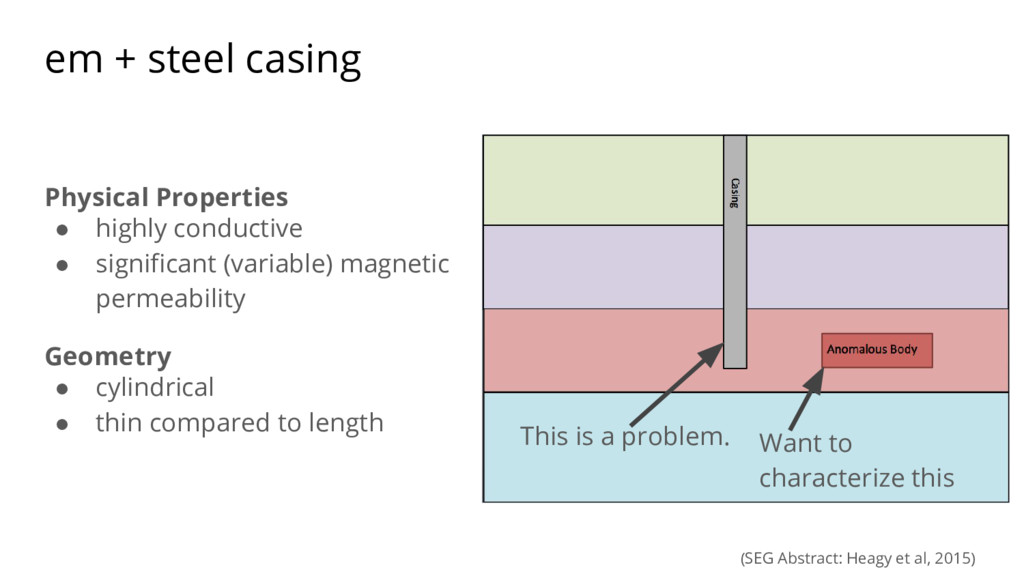
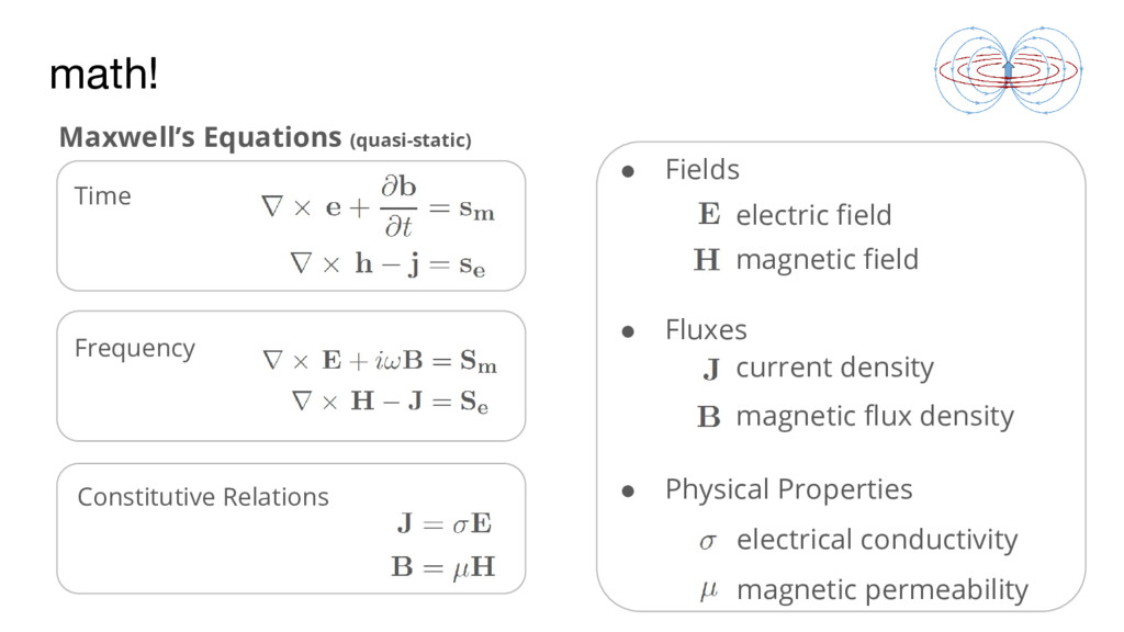
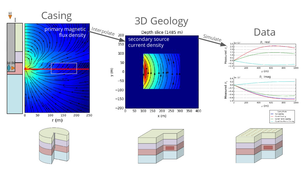
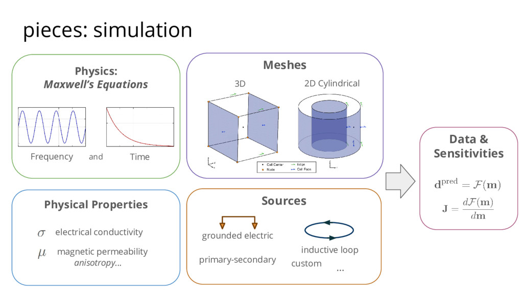
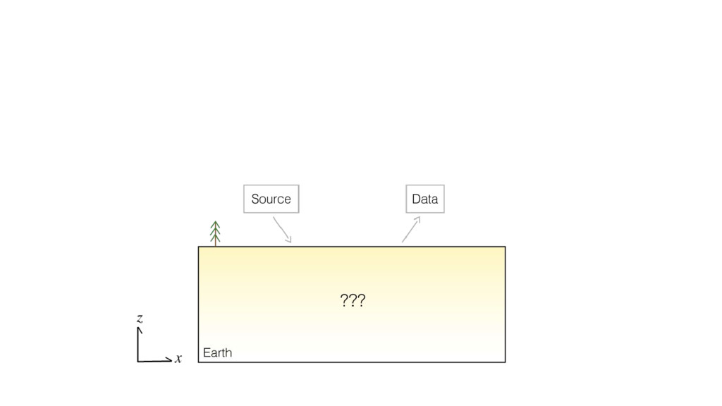
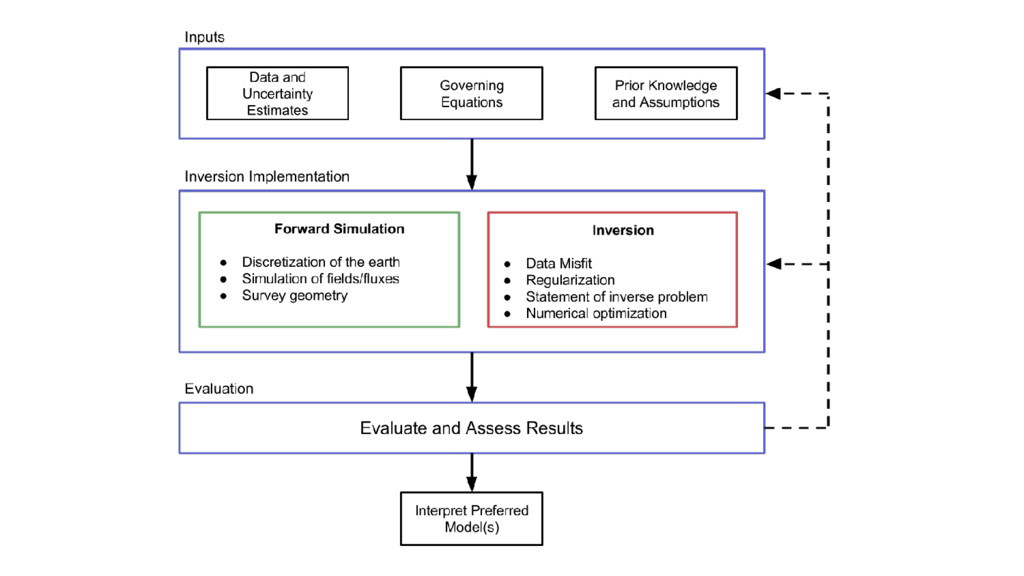
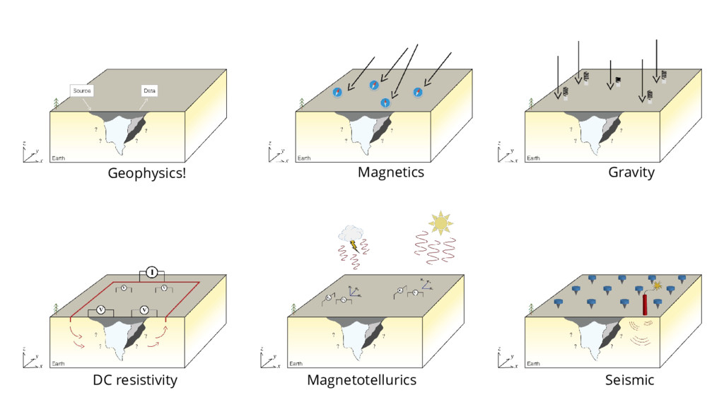
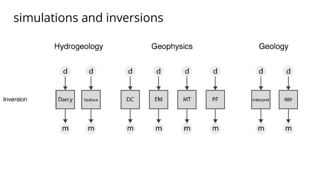
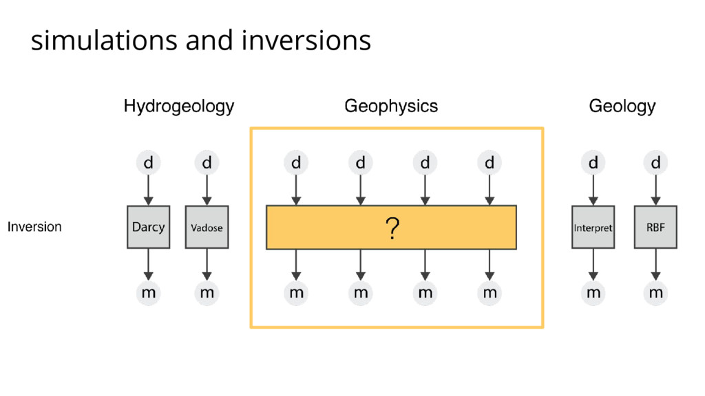
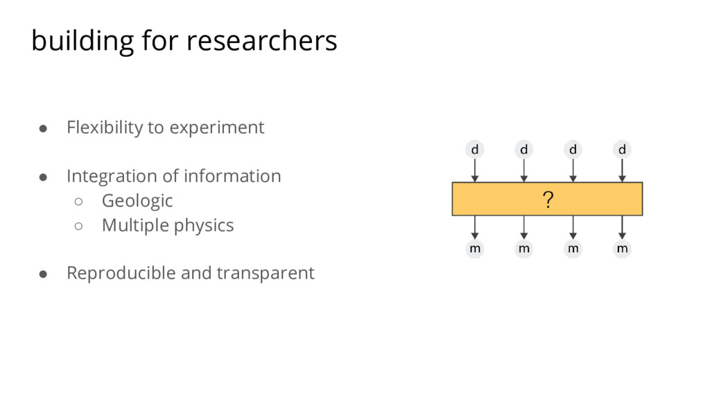
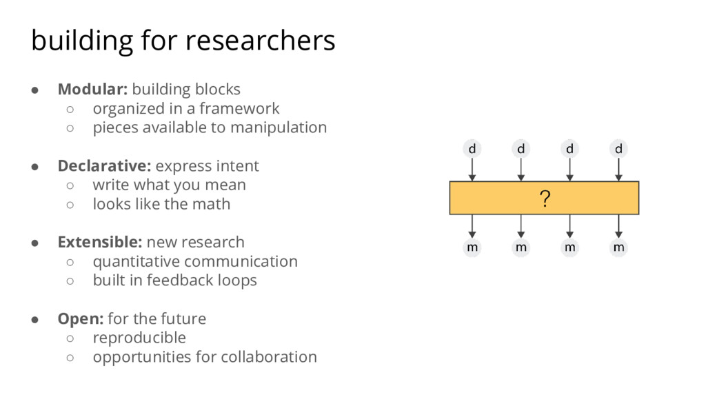
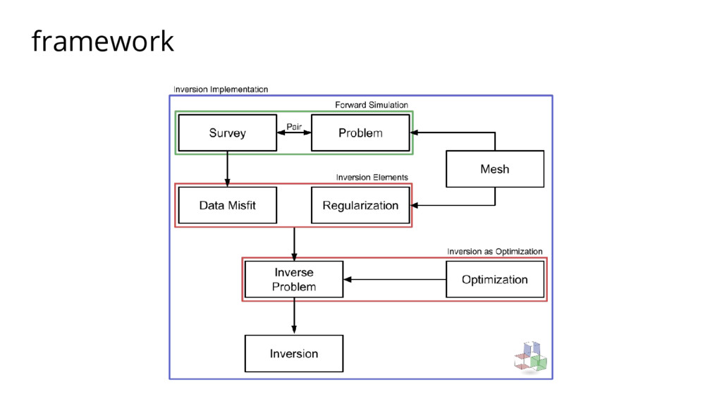
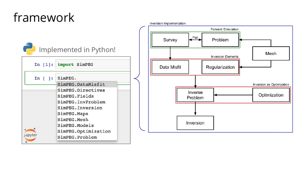
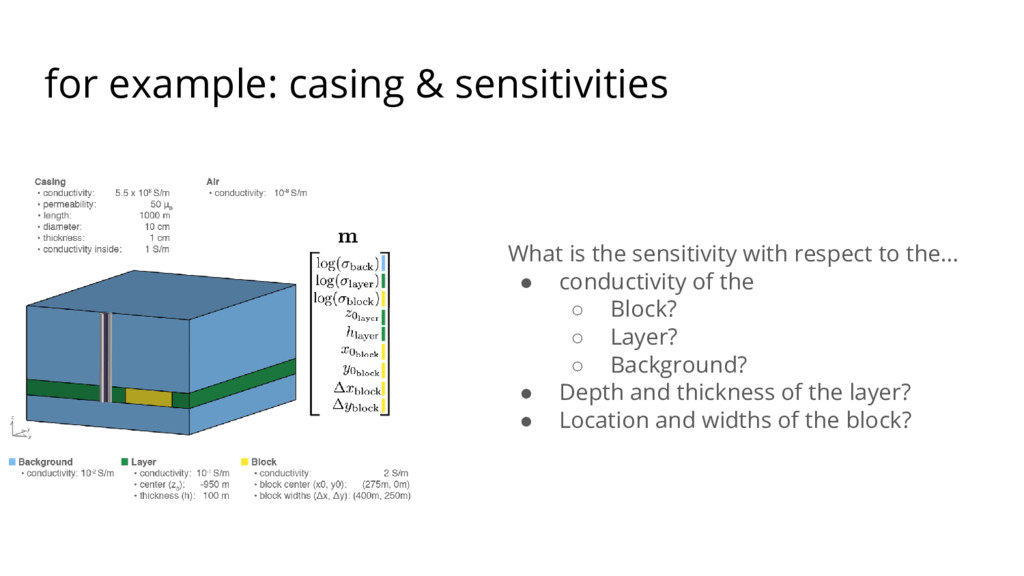
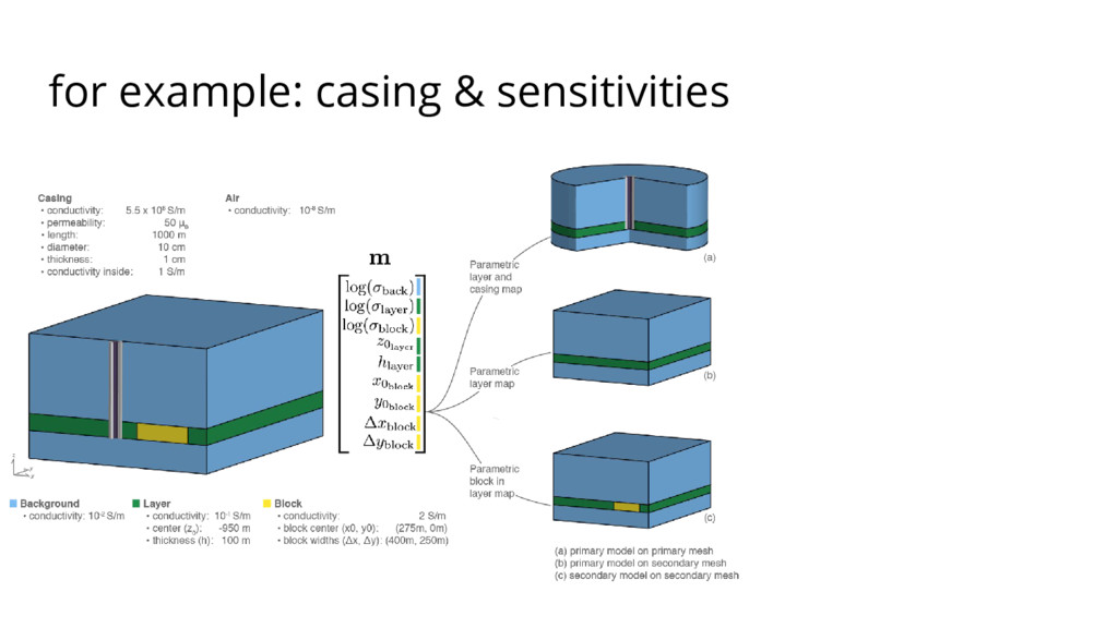
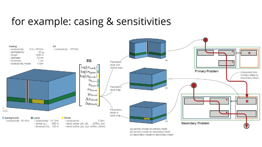
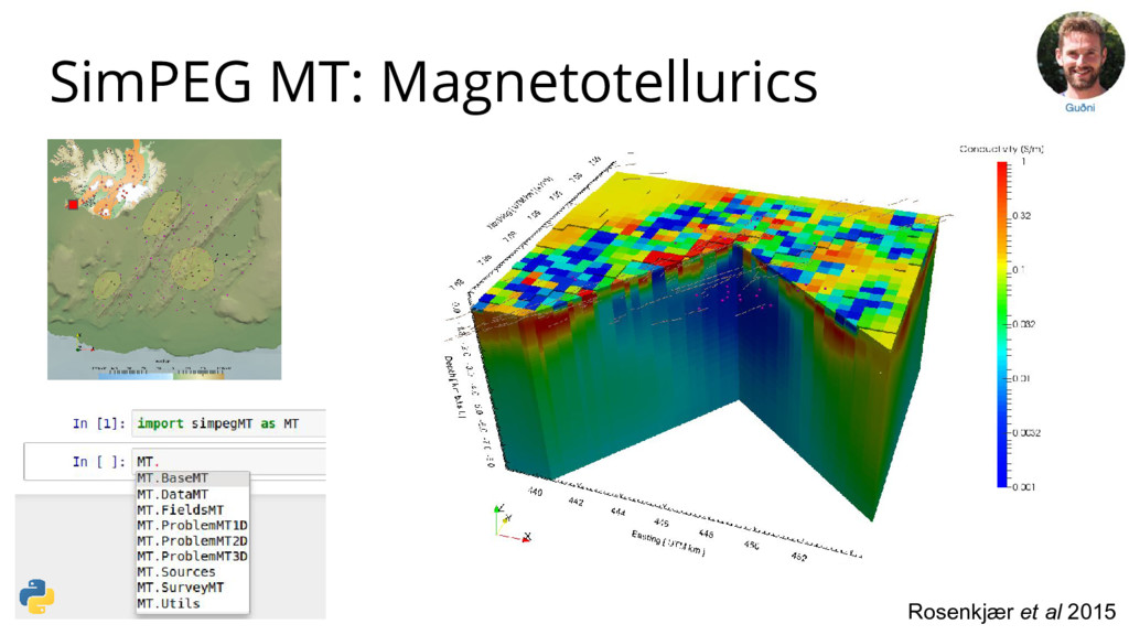
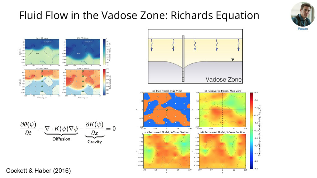
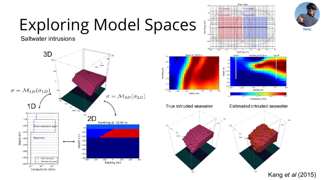
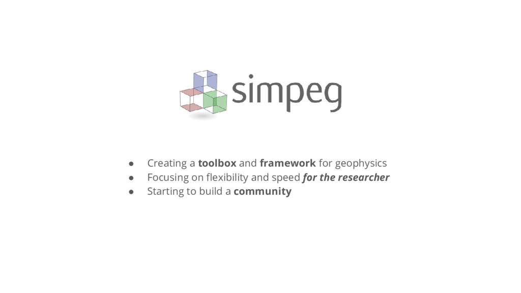
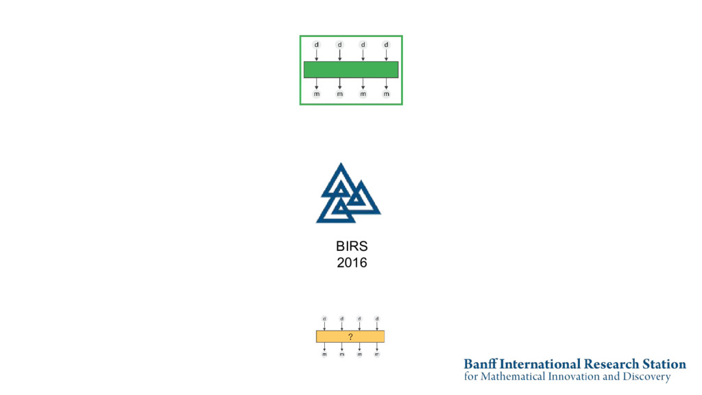
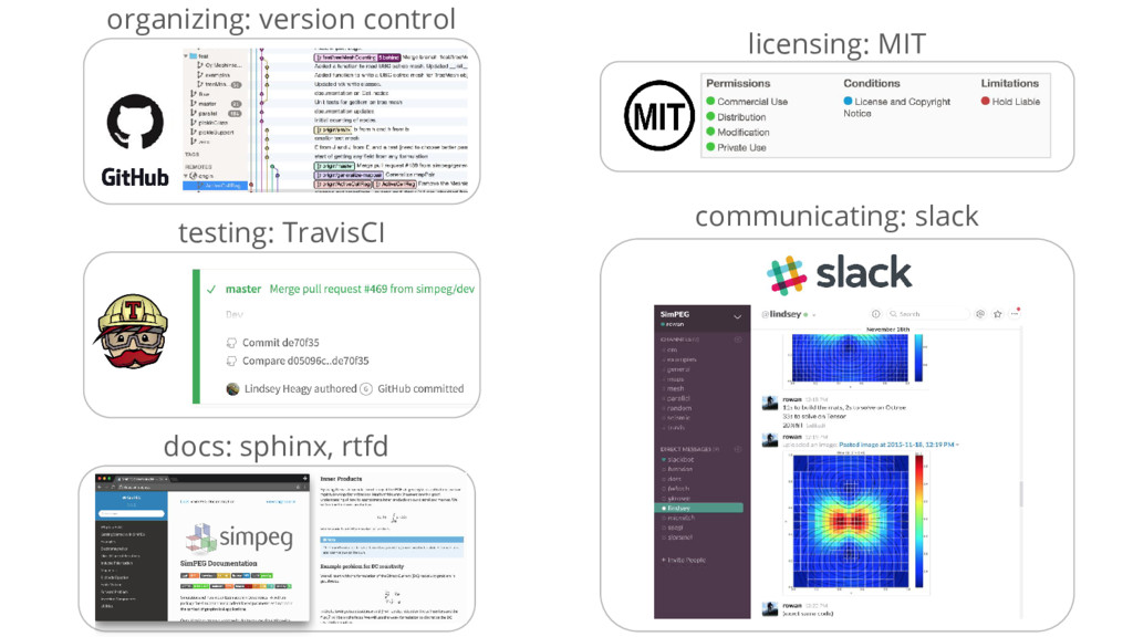
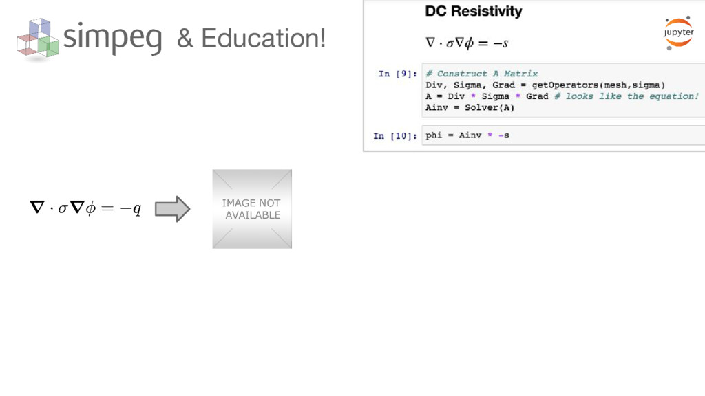
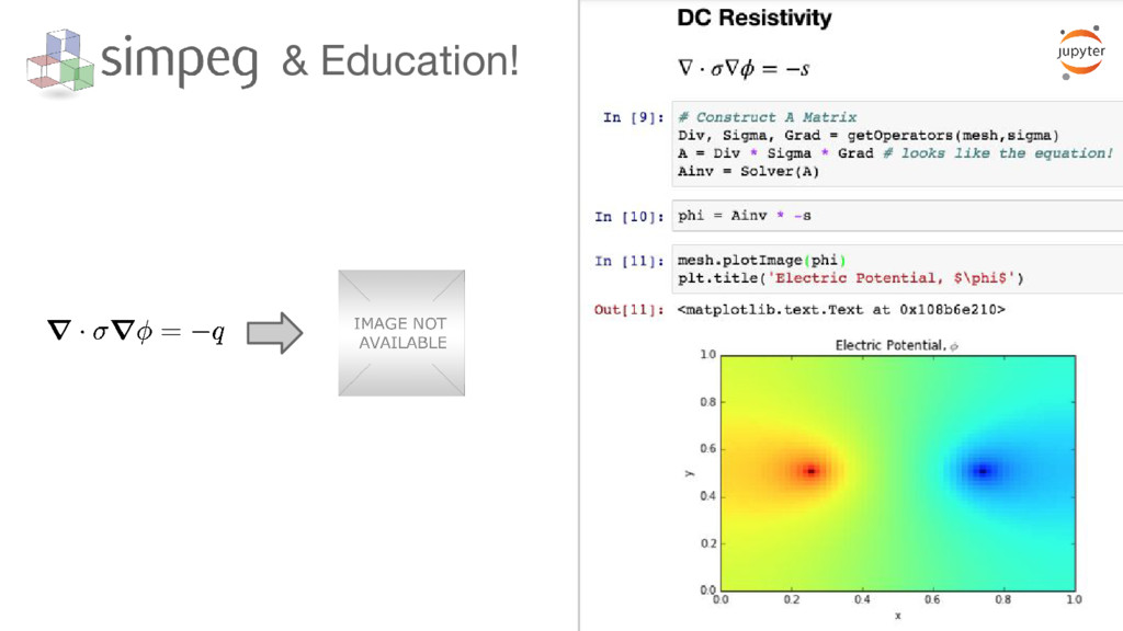
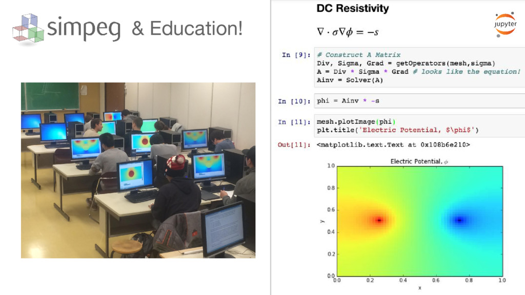
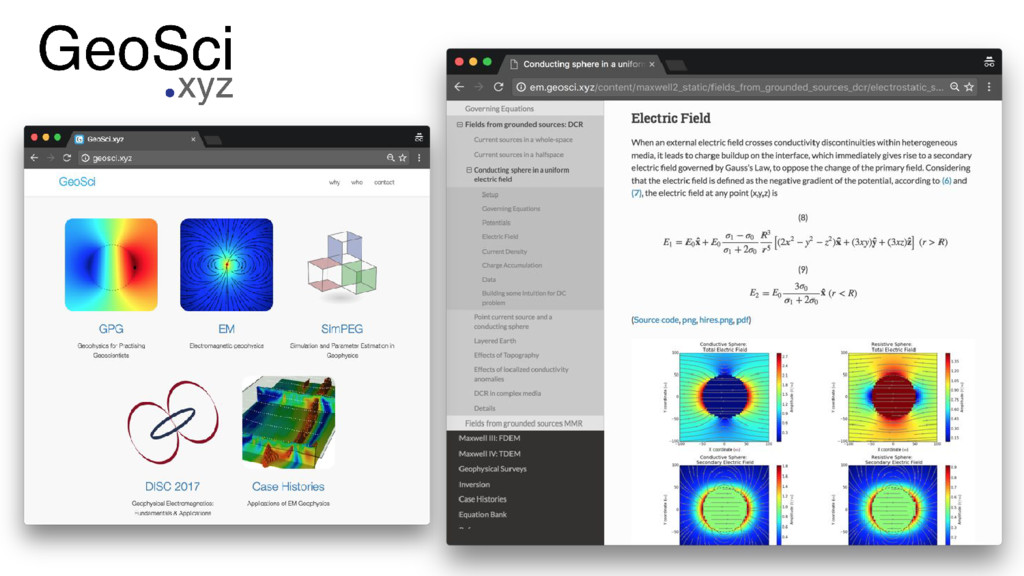
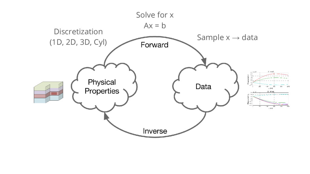
Geophysical inverse problems are used to estimate models of the subsurface from a finite number of data collected over the earth. SimPEG (Simulation and Parameter Estimation in Geophysics, http://simpeg.xyz) is a collaborative effort to develop an open source framework for solving geophysical simulation and inversion problems, including electromagnetics, vadose zone flow, and potential fields, in a consistent manner. The goal in the development of SimPEG is to support a community of researchers with well-tested, extensible tools, and encourage transparency and reproducibility both of the SimPEG software and the geoscientific research it is applied to. Using an example from applied electromagnetics: monitoring an injection (such as a hydraulic fracturing) from a steel cased well, I will provide an overview of the framework and discuss some of the strategies we are using to promote collaboration. I will also discuss how we have re-purposed the numerical tools in SimPEG to build web-based interactive simulations for students to explore fundamental concepts in geophysics (http://geosci.xyz).

Transcript

1. open source simulations and inversions in geophysics Lindsey Heagy with Rowan Cockett, Seogi Kang, Doug Oldenburg, Gudni Rosenkaer, Dom Fournier, et al Geophysical Inversion Facility University of British Columbia
2. • Context: an applied EM problem ◦ An example: steel casing • Big picture: simulations and inversions in geophysics ◦ What are the pieces? • Framework & Toolbox ◦ How do we implement this? • Building in the open ◦ What can I do with it? ◦ Collaborative development • Interactive geophysics ◦ Teaching with numerical simulations outline
3. em? Electrical conductivity can be diagnostic for…
4. em + steel casing This is a problem. Want to characterize this (SEG Abstract: Heagy et al, 2015) Physical Properties • highly conductive • significant (variable) magnetic permeability Geometry • cylindrical • thin compared to length
5. • Fields magnetic flux density current density • Physical Properties • Fluxes Constitutive Relations Maxwell’s Equations (quasi-static) electric field magnetic field electrical conductivity magnetic permeability Time Frequency math!
6. primary magnetic flux density Interpolate secondary source current density Casing 3D Geology Data Simulate
7. grounded electric Physics: Maxwell’s Equations Physical Properties electrical conductivity magnetic permeability anisotropy... Meshes 2D Cylindrical Sources inductive loop primary-secondary Data & Sensitivities … and Time Frequency 3D custom pieces: simulation
8. inverse problems
11. Magnetics Gravity DC resistivity Magnetotellurics Seismic Geophysics!
12. simulations and inversions
13. simulations and inversions
14. building for researchers • Flexibility to experiment • Integration of information ◦ Geologic ◦ Multiple physics • Reproducible and transparent
15. • Modular: building blocks ◦ organized in a framework ◦ pieces available to manipulation • Declarative: express intent ◦ write what you mean ◦ looks like the math • Extensible: new research ◦ quantitative communication ◦ built in feedback loops • Open: for the future ◦ reproducible ◦ opportunities for collaboration building for researchers
16. building for researchers • Modular: building blocks ◦ organized in a framework ◦ pieces available to manipulation • Declarative: express intent ◦ write what you mean ◦ looks like the math • Extensible: new research ◦ quantitative communication ◦ built in feedback loops • Open: for the future ◦ reproducible ◦ opportunities for collaboration
17. framework
18. Implemented in Python! framework
19. forward simulation Survey: Data collection and geometry Problem: Physics
20. finite volume
21. create a mesh
22. • Fields • Fluxes • Physical Properties discretize electric field magnetic field magnetic flux density current density electrical conductivity magnetic permeability
23. solve continuous discrete
24. framework
25. Data Misfit Regularization Inverse Problem inversion elements
26. inversion as optimization
27. For second order optimization techniques, need data: And sensitivities: sensitivities
28. forward simulation & sensitivities
29. Forward Inverse
31. ?
32. Model & Physical Properties: What should we invert for? (SEG Abstract: Kang et al, 2015) Derivatives using chain rule: or : • Active reservoir layer • Parametric representation • ... inversion model physical properties
33. ?
34. grounded electric inductive loop point dipole (electric or magnetic) fields from a primary problem natural source Sources: How do we excite the Earth?
35. ?
36. Solve 2nd order system Solve E-B, H-J ? or and compute derivative Physics: How do we solve Maxwell’s equations
37. ?
38. compute fields everywhere: what we solved for from source derivative Fields: How do we calculate the EM fields and fluxes? from source from physics
39. ?
40. ... Data: Receivers: What, and where, do we measure?
41. Plug in the pieces
42. Sensitivities
43. How do we know it works? Testing! • Taylor series
44. for example: casing & sensitivities What is the sensitivity with respect to the… • conductivity of the ◦ Block? ◦ Layer? ◦ Background? • Depth and thickness of the layer? • Location and widths of the block? Heagy et al. 2016 - in review
45. for example: casing & sensitivities What is the sensitivity with respect to the… • conductivity of the ◦ Block? ◦ Layer? ◦ Background? • Depth and thickness of the layer? • Location and widths of the block?
46. for example: casing & sensitivities
47. for example: casing & sensitivities
48. data
49. sensitivities • Need background model • Collect data away from the
50. sensitivities • Need background model • Collect data away from the source (up to ~1 km away)
51. summary • Modular, composable pieces ◦ Compartmentalize concerns ◦ All pieces available to manipulation → extensible • Testing! ◦ Test pieces ◦ Test composite http://www.flickr.com/photos/13403905@N03/2080281038/
52. Building in the open
53. Heagy et al. 2016 - in review
54. Heagy et al. 2016 - in review
55. Magnetics Gravity DC resistivity Magnetotellurics Seismic Geophysics!
56. DC Resistivity
57. Potential Fields: Gravity & Magnetics
58. Airborne Time Domain EM Inversion Figure above shows plan views of (a) the true conductivity model and (b) the recovered model, and section views of (c) the true and (d) the recovered conductivity models. Figure to the left shows observed and predicted data. Core cell size: 50×50×20 m, The number of cell: 50×50×48 = 120,000; Reference model: Half-space model with conductivity value, 0.005 S/m; Inexact Gauss-Newton: 13 iterations; Cpu time: 48hrs; Maximum memory usage: 51.2GB; Cpu:Intel(R)Xeon(R) CPU 2.80 GHz; Ram: 64 GB
59. SimPEG MT: Magnetotellurics Rosenkjær et al 2015
60. Fluid Flow in the Vadose Zone: Richards Equation Cockett & Haber (2016)
61. Exploring Model Spaces Saltwater intrusions Kang et al (2015)
62. • Creating a toolbox and framework for geophysics • Focusing on flexibility and speed for the researcher • Starting to build a community
63. BIRS 2016
64. strategies for open, collaborative development
65. communicating: slack testing: TravisCI organizing: version control docs: sphinx, rtfd licensing: MIT
66. using numerical tools in education
67. & Education!
68. & Education!
69. & Education!
71. thank you! simpeg.xyz geosci.xyz lheagy@eos.ubc.ca @
73. Discretization (1D, 2D, 3D, Cyl) Solve for x Ax = b Sample x → data
74. Lindsey Heagy with : Geophysical Inversion Facility University of British Columbia
75. about me • Grad studies in geophysics ◦ Computational