Minimizing the Number of Edges via Edge Concentration in Dense Layered Graphs

IEEE Pacific Vis 2016

Transcript

1. Minimizing the Number of Edges via Edge Concentration in Dense Layered Graphs Yosuke Onoue 1), Nobuyuki Kukimoto 1), Naohisa Sakamoto 2), and Koji Koyamada 1) 1) Kyoto University, 2) Kobe University
2. Introduction
3. Layered Drawing • Drawing technique for visualizing the hierarchical structures of directed graphs G = (V, E) • Sugiyama framework (Sugiyama 1981)
4. Layered Drawing for Dense Graphs • Dense graphs have many edge crossings • Visual clutter • Difficult to understand graphs • Crossing reduction has a limitation • Unavoidable edge crossing
 e.g. biclique (complete bipartite graph) K22 X Y A B
5. Edge Concentration (EC) • Optional process for layered drawing • Replace bicliques with concentration vertices
 in bipartite graph G = (U, L, E) • Reduce edge crossings • Newbery’s algorithm (Newbery 1989) X Y Z A B C A B C X 1 1 0 Y 1 1 1 Z 0 1 1 A B C X Y Z Input Output Adjacency matrix
6. Challenge • Existing algorithm sometimes fails to simplify graphs • More efficient algorithm is needed A B C D E W 1 1 1 0 1 X 1 1 1 1 0 Y 0 1 1 1 1 Z 1 0 1 1 1 Adjacency matrix w x y A B C Input z D E 16 edges, 28 crossings Output w x y A B C z D E 30 edges, 42 crossings The number of crossings increases !
7. Related Work • Edge Bundling • EC changes graph topology • Confluent Layered Drawing (Eppstein2007) • Crossing-free layout • Semantic Edge Bundling (Sun2016) • Using biclustering • No novel EC algorithm has been developed D. Eppstein, M. T. Goodrich, and J. Y. Meng, “Confluent Layered Drawings,” Algorithmica, vol. 47, no. 4, pp. 439–452, Apr. 2007. M. Sun, P. Mi, C. North, and N. Ramakrishnan, “BiSet: Semantic Edge Bundling with Biclusters for Sensemaking.,” IEEE Trans. Vis. Comput. Graph., vol. 22, no. 1, pp. 310–9, Jan. 2016.
8. Proposed Method
9. Approach • Minimize the number of edges after EC • Replacing Knm reduces
 (n * m - n - m) edges • Some edges contained in multiple bicliques |E| = 12 X Y Z A B C D E A B C D E X 1 1 1 0 1 Y 1 1 1 1 0 Z 0 1 1 1 1 Input |E| = 15 A B C D E X Y Z A B C D E X 1 1 1 0 1 Y 1 1 1 1 0 Z 0 1 1 1 1 Newbery’s method |E| = 11 X Y Z A B C D E A B C D E X 1 1 1 0 1 Y 1 1 1 1 0 Z 0 1 1 1 1 Minimum edge number 11 edges 10 edges (1 duplicate path)
10. Heuristic Algorithm • MaxRect • Finding maximum rectangular region that reduces the number of edges in an adjacency matrix repeatedly • O(|E||U||L|) C A B D E W 1 1 1 0 1 X 1 1 1 1 0 Y 1 0 1 1 1 Z 1 1 0 1 1 D E C A B Y 1 1 1 0 1 Z 1 1 1 1 0 W 0 1 1 1 1 X 1 0 1 1 1 A B D E C W 1 1 0 1 1 X 1 1 1 0 1 Y 0 1 1 1 1 Z 1 0 1 1 1 Increasing order of out-degree Maximum rectangular region Replaced edges No more edge concentration that reduces the number of edges. Stop. w x y A B C z D E 15 edges, 16 crossings
11. Computational Experiments
12. Comparison • Proposed method vs Newbery’s method • Number of edges • Number of crossings • Number of concentration vertices • Computation time • Randomly generated bipartite graphs • |U|, |L| ∈ {5, 10, 15, 20}, p ∈ {0.7, 0.8, 0.9}, |U| < |L| • 30 instances for each (|U|, |L|, p) • Environment • Laptop PC (Mac OS X, 2.8 GHz Intel CPU, 16GB RAM)
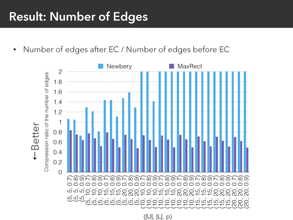
13. Result: Number of Edges • Number of edges after EC / Number of edges before EC Compression ratio of the number of edges 0 0.2 0.4 0.6 0.8 1 1.2 1.4 1.6 1.8 2 (|U|, |L|, p) (5, 5, 0.7) (5, 5, 0.8) (5, 5, 0.9) (5, 10, 0.7) (5, 10, 0.8) (5, 10, 0.9) (5, 15, 0.7) (5, 15, 0.8) (5, 15, 0.9) (5, 20, 0.7) (5, 20, 0.8) (5, 20, 0.9) (10, 10, 0.7) (10, 10, 0.8) (10, 10, 0.9) (10, 15, 0.7) (10, 15, 0.8) (10, 15, 0.9) (10, 20, 0.7) (10, 20, 0.8) (10, 20, 0.9) (15, 15, 0.7) (15, 15, 0.8) (15, 15, 0.9) (15, 20, 0.7) (15, 20, 0.8) (15, 20, 0.9) (20, 20, 0.7) (20, 20, 0.8) (20, 20, 0.9) Newbery MaxRect ←Better
14. Result: Number of Crossings • Number of crossings after EC / Number of crossings before EC Compression ratio of the number of crossings 0 0.2 0.4 0.6 0.8 1 1.2 1.4 1.6 1.8 2 (|U|, |L|, p) (5, 5, 0.7) (5, 5, 0.8) (5, 5, 0.9) (5, 10, 0.7) (5, 10, 0.8) (5, 10, 0.9) (5, 15, 0.7) (5, 15, 0.8) (5, 15, 0.9) (5, 20, 0.7) (5, 20, 0.8) (5, 20, 0.9) (10, 10, 0.7) (10, 10, 0.8) (10, 10, 0.9) (10, 15, 0.7) (10, 15, 0.8) (10, 15, 0.9) (10, 20, 0.7) (10, 20, 0.8) (10, 20, 0.9) (15, 15, 0.7) (15, 15, 0.8) (15, 15, 0.9) (15, 20, 0.7) (15, 20, 0.8) (15, 20, 0.9) (20, 20, 0.7) (20, 20, 0.8) (20, 20, 0.9) Newbery MaxRect ←Better
15. Result: Number of Concentration Vertices Number of concentration vertices 0 2 4 6 8 10 12 14 16 18 20 (|U|, |L|, p) (5, 5, 0.7) (5, 5, 0.8) (5, 5, 0.9) (5, 10, 0.7) (5, 10, 0.8) (5, 10, 0.9) (5, 15, 0.7) (5, 15, 0.8) (5, 15, 0.9) (5, 20, 0.7) (5, 20, 0.8) (5, 20, 0.9) (10, 10, 0.7) (10, 10, 0.8) (10, 10, 0.9) (10, 15, 0.7) (10, 15, 0.8) (10, 15, 0.9) (10, 20, 0.7) (10, 20, 0.8) (10, 20, 0.9) (15, 15, 0.7) (15, 15, 0.8) (15, 15, 0.9) (15, 20, 0.7) (15, 20, 0.8) (15, 20, 0.9) (20, 20, 0.7) (20, 20, 0.8) (20, 20, 0.9) Newbery MaxRect
16. Result: Computation Time ←Better Computation time (milliseconds) 0 2 4 6 8 10 12 14 16 18 20 (|U|, |L|, p) (5, 5, 0.7) (5, 5, 0.8) (5, 5, 0.9) (5, 10, 0.7) (5, 10, 0.8) (5, 10, 0.9) (5, 15, 0.7) (5, 15, 0.8) (5, 15, 0.9) (5, 20, 0.7) (5, 20, 0.8) (5, 20, 0.9) (10, 10, 0.7) (10, 10, 0.8) (10, 10, 0.9) (10, 15, 0.7) (10, 15, 0.8) (10, 15, 0.9) (10, 20, 0.7) (10, 20, 0.8) (10, 20, 0.9) (15, 15, 0.7) (15, 15, 0.8) (15, 15, 0.9) (15, 20, 0.7) (15, 20, 0.8) (15, 20, 0.9) (20, 20, 0.7) (20, 20, 0.8) (20, 20, 0.9) Newbery MaxRect
17. Drawing Results
18. Application Example
19. Real-world Application • Visualization of observed data in the embryogenesis of the nematode C. elegans obtained from the WDDD (Worm Developmental Dynamics Database) K. Kyoda et al. “WDDD: Worm Developmental Dynamics Database.” Nucleic acids research, vol. 41, no. Database issue, pp. D732–7, jan 2013. https://en.wikipedia.org/wiki/Caenorhabditis_elegans
20. Visual Representation 1 cell 1-2 cell 2 cells Time … … Nucleus volume Nucleus position Distance between 2 nuclei Variable Type An edge from X to Y 㱺 |correlation between X and Y| > threshold X Y
21. Drawing Result (a) without edge concentration (b) with edge concentration 16 concentration vertices are inserted, the number of edges reduced by 11 % 179 vertices, 329 edges 195 vertices, 294 edges
22. Drawing Result (a) without edge concentration (b) with edge concentration
23. Conclusion
24. Conclusion • We proposed a novel edge concentration method • Approach based on minimizing the total number of edges after edge concentration • Proposed method has advantage over the simplification performance compared to the existing method • Efficiency of the proposed method is demonstrated in application example
25. Future Work • Developing an exact solution method • To evaluate the relative performance of the heuristic method • Conducting a formal user study • To assess the user performance • Applying to other application fields • Software visualization • Citation network
28. Drawing Result (4cell, 4-8cell, 8cell)