Black Scholes Model

Mathematical study of black and scholes model.

Transcript

1. Mathematical Study of Black-Scholes Model Luckshay Batra luckybatra17@gmail.com
2. Table of content Black-Scholes Model • Introduction • Key terms • Black Scholes Formula • Black Scholes Calculators • Wiener Process • Stock Pricing Model • Ito’s Lemma • Derivation of Black-Sholes Equation • Solution of Black-Scholes Equation • Maple solution of Black Scholes Equation • Figures Option Pricing with Transaction costs and Stochastic Volatility • Introduction • Key terms • Stochastic Volatility Model Quanto Option Pricing Model • Key Terms • Pricing Quantos in Excel • Black-Scholes Equation of Quanto options • Solution of Quanto options Black-Scholes Equation
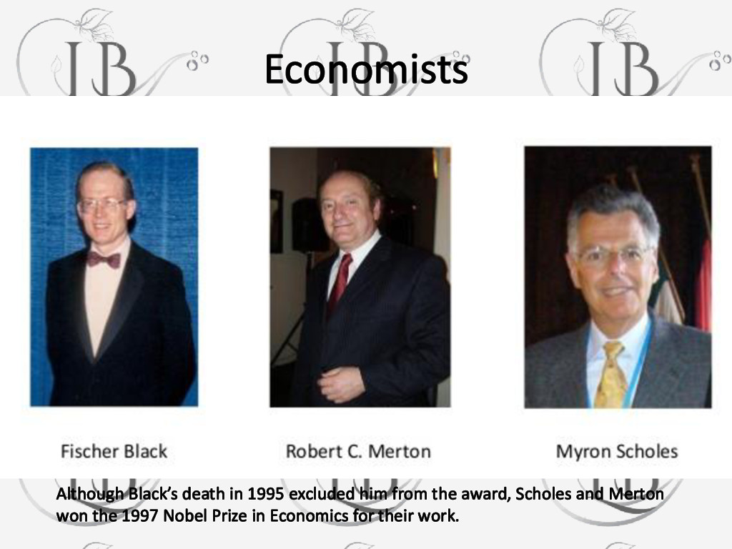
3. Introduction  A model of price variation over time of financial instruments such as stocks that can, among other things, be used to determine the price of a European call option & American option.  The Black Scholes Model is one of the most important concepts in modern financial theory.  It was developed in 1973 by Fisher Black, Robert Merton and Myron Scholes and is still widely used today, and regarded as one of the best ways of determining fair prices of options.  Also known as the Black-Scholes-Merton Model.
4. Economists Although Black’s death in 1995 excluded him from the award, Scholes and Merton won the 1997 Nobel Prize in Economics for their work.
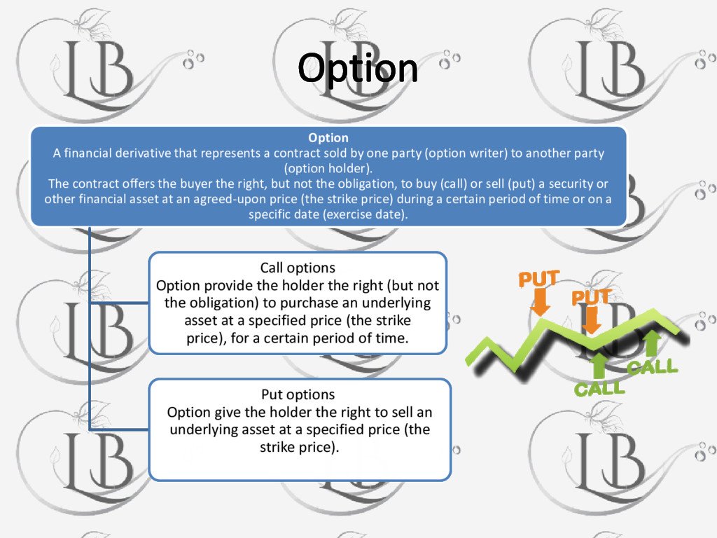
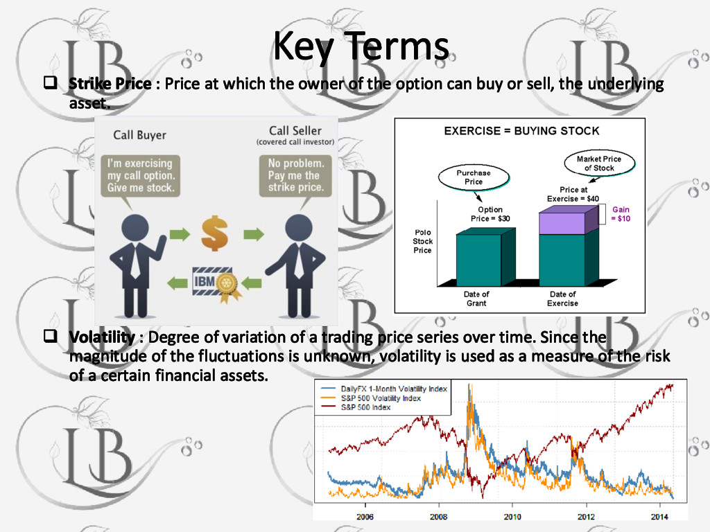
5. Option Option A financial derivative that represents a contract sold by one party (option writer) to another party (option holder). The contract offers the buyer the right, but not the obligation, to buy (call) or sell (put) a security or other financial asset at an agreed-upon price (the strike price) during a certain period of time or on a specific date (exercise date). Call options Option provide the holder the right (but not the obligation) to purchase an underlying asset at a specified price (the strike price), for a certain period of time. Put options Option give the holder the right to sell an underlying asset at a specified price (the strike price).
6. Key Terms  Strike Price : Price at which the owner of the option can buy or sell, the underlying asset.  Volatility : Degree of variation of a trading price series over time. Since the magnitude of the fluctuations is unknown, volatility is used as a measure of the risk of a certain financial assets.
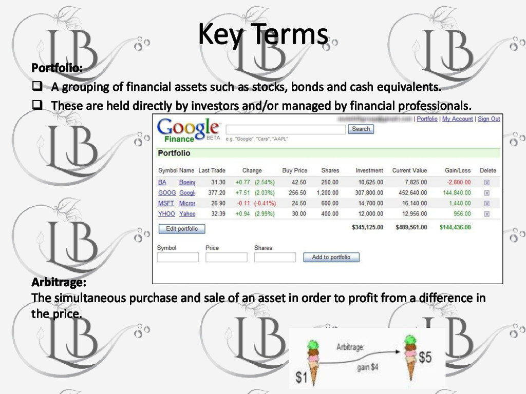
7. Key Terms Portfolio:  A grouping of financial assets such as stocks, bonds and cash equivalents.  These are held directly by investors and/or managed by financial professionals. Arbitrage: The simultaneous purchase and sale of an asset in order to profit from a difference in the price.
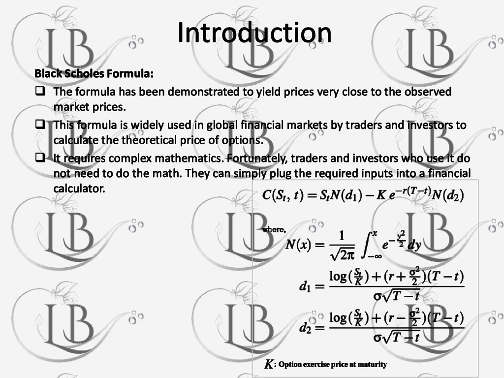
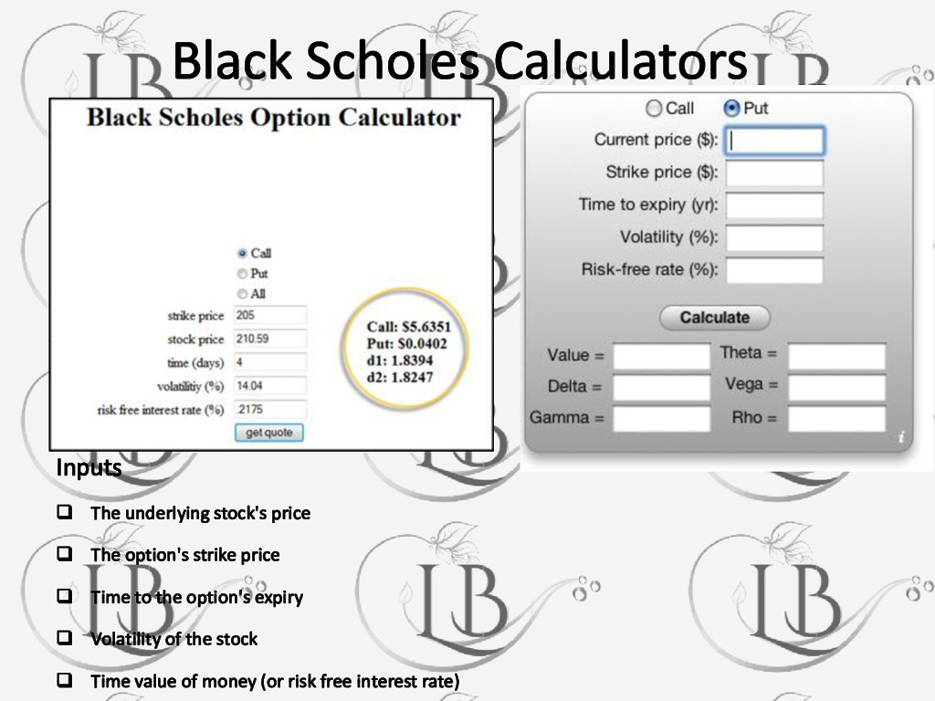
8. Introduction Black Scholes Formula:  The formula has been demonstrated to yield prices very close to the observed market prices.  This formula is widely used in global financial markets by traders and investors to calculate the theoretical price of options.  It requires complex mathematics. Fortunately, traders and investors who use it do not need to do the math. They can simply plug the required inputs into a financial calculator.
9. Black Scholes Calculators Inputs  The underlying stock's price  The option's strike price  Time to the option's expiry  Volatility of the stock  Time value of money (or risk free interest rate)
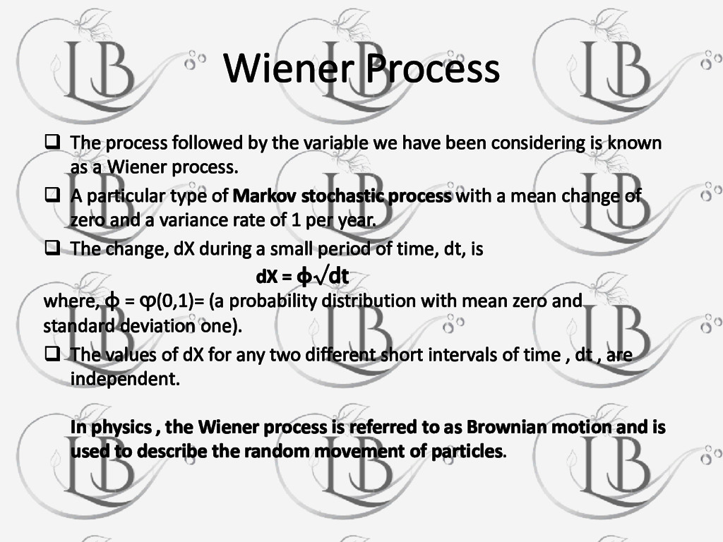
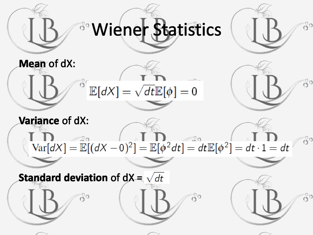
10. Wiener Process  The process followed by the variable we have been considering is known as a Wiener process.  A particular type of Markov stochastic process with a mean change of zero and a variance rate of 1 per year.  The change, dX during a small period of time, dt, is dX = φ√dt where, φ = ϕ(0,1)= (a probability distribution with mean zero and standard deviation one).  The values of dX for any two different short intervals of time , dt , are independent. In physics , the Wiener process is referred to as Brownian motion and is used to describe the random movement of particles.
11. Wiener Statistics Mean of dX: Variance of dX: Standard deviation of dX =
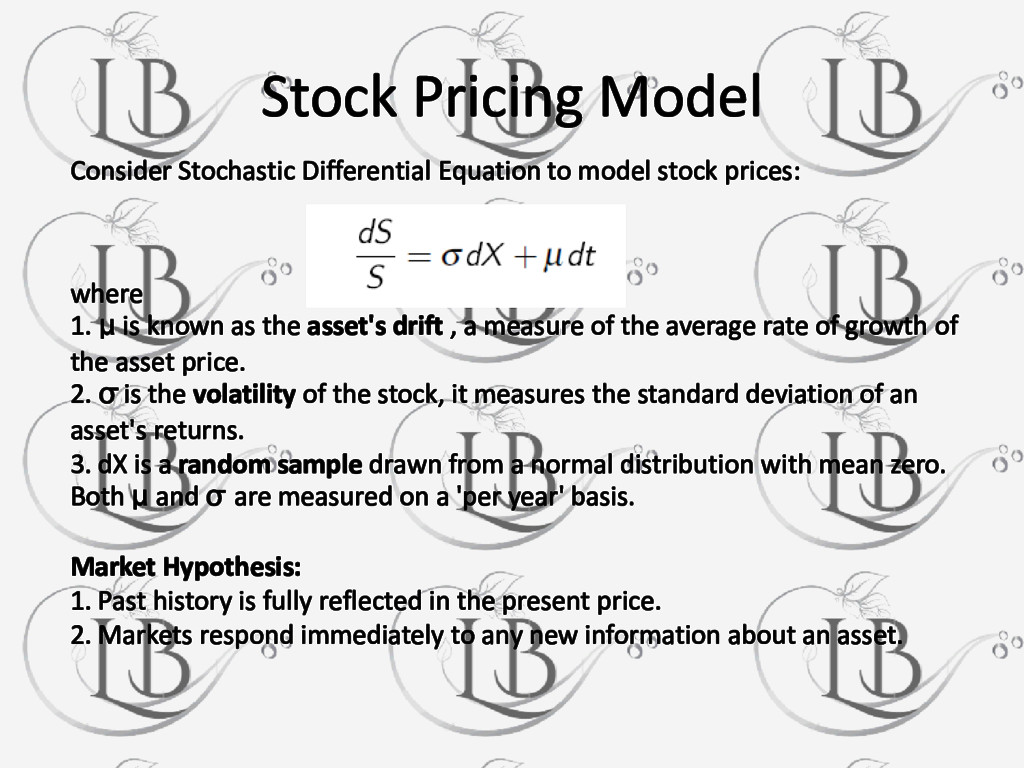
12. Stock Pricing Model Consider Stochastic Differential Equation to model stock prices: where 1. μ is known as the asset's drift , a measure of the average rate of growth of the asset price. 2. σ is the volatility of the stock, it measures the standard deviation of an asset's returns. 3. dX is a random sample drawn from a normal distribution with mean zero. Both μ and σ are measured on a 'per year' basis. Market Hypothesis: 1. Past history is fully reflected in the present price. 2. Markets respond immediately to any new information about an asset.
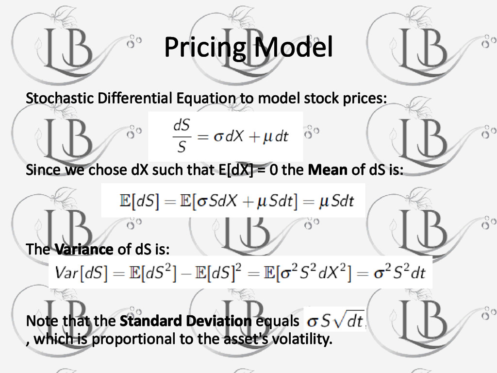
13. Pricing Model Stochastic Differential Equation to model stock prices: Since we chose dX such that E[dX] = 0 the Mean of dS is: The Variance of dS is: Note that the Standard Deviation equals , which is proportional to the asset's volatility.
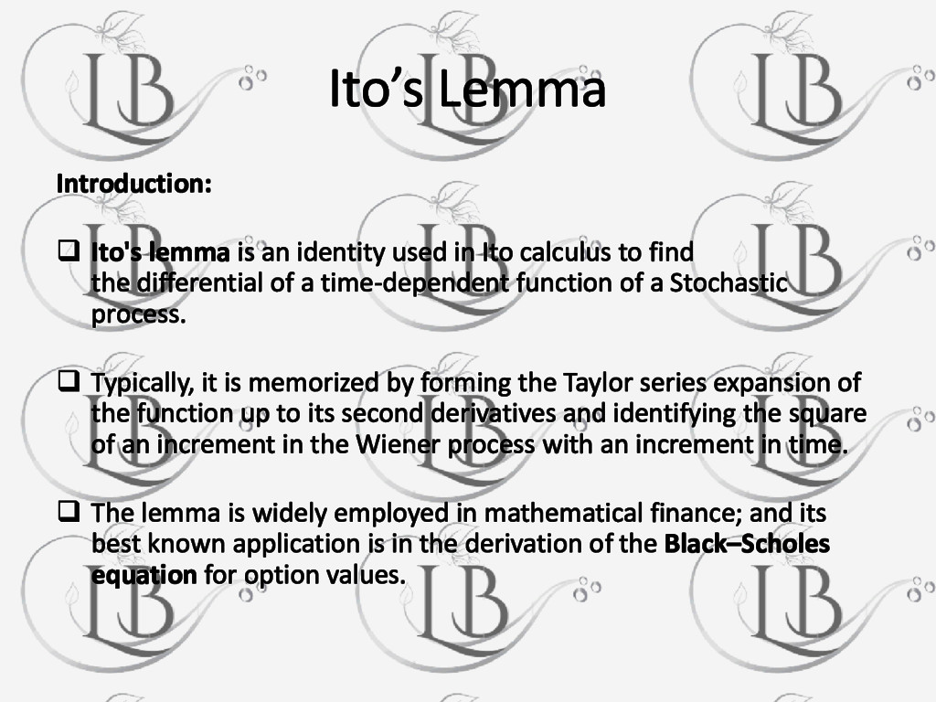
14. Ito’s Lemma Introduction:  Ito's lemma is an identity used in Ito calculus to find the differential of a time-dependent function of a Stochastic process.  Typically, it is memorized by forming the Taylor series expansion of the function up to its second derivatives and identifying the square of an increment in the Wiener process with an increment in time.  The lemma is widely employed in mathematical finance; and its best known application is in the derivation of the Black–Scholes equation for option values.
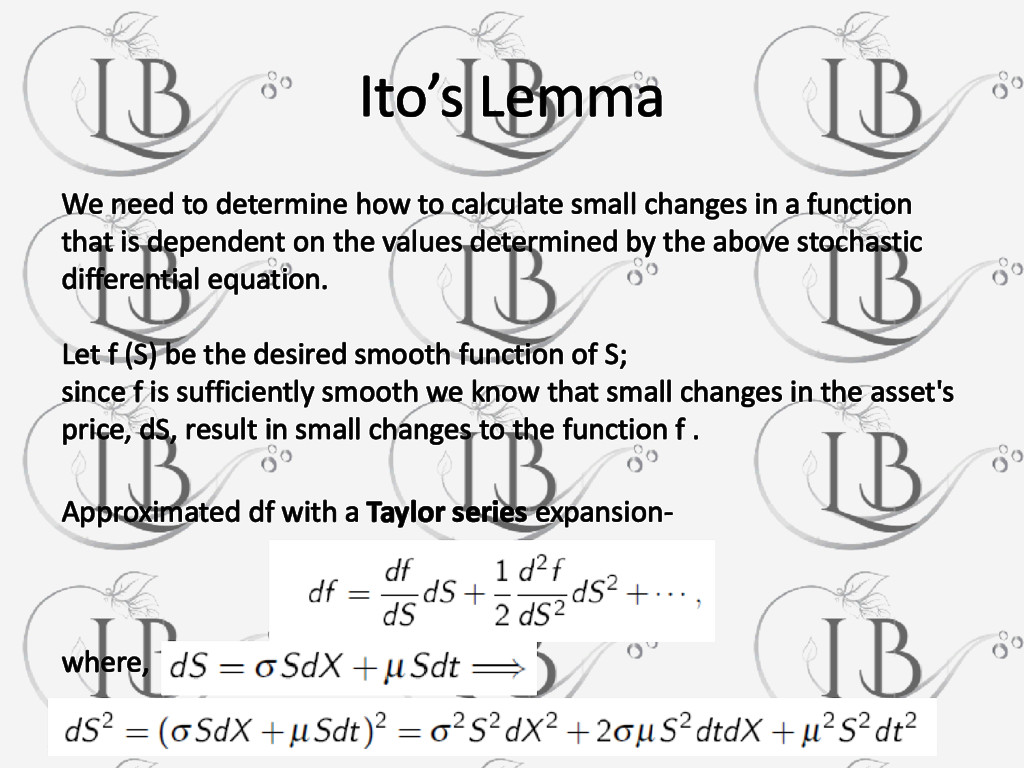
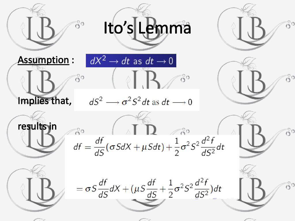
15. Ito’s Lemma We need to determine how to calculate small changes in a function that is dependent on the values determined by the above stochastic differential equation. Let f (S) be the desired smooth function of S; since f is sufficiently smooth we know that small changes in the asset's price, dS, result in small changes to the function f . Approximated df with a Taylor series expansion- where,
16. Ito’s Lemma Assumption : Implies that, results in
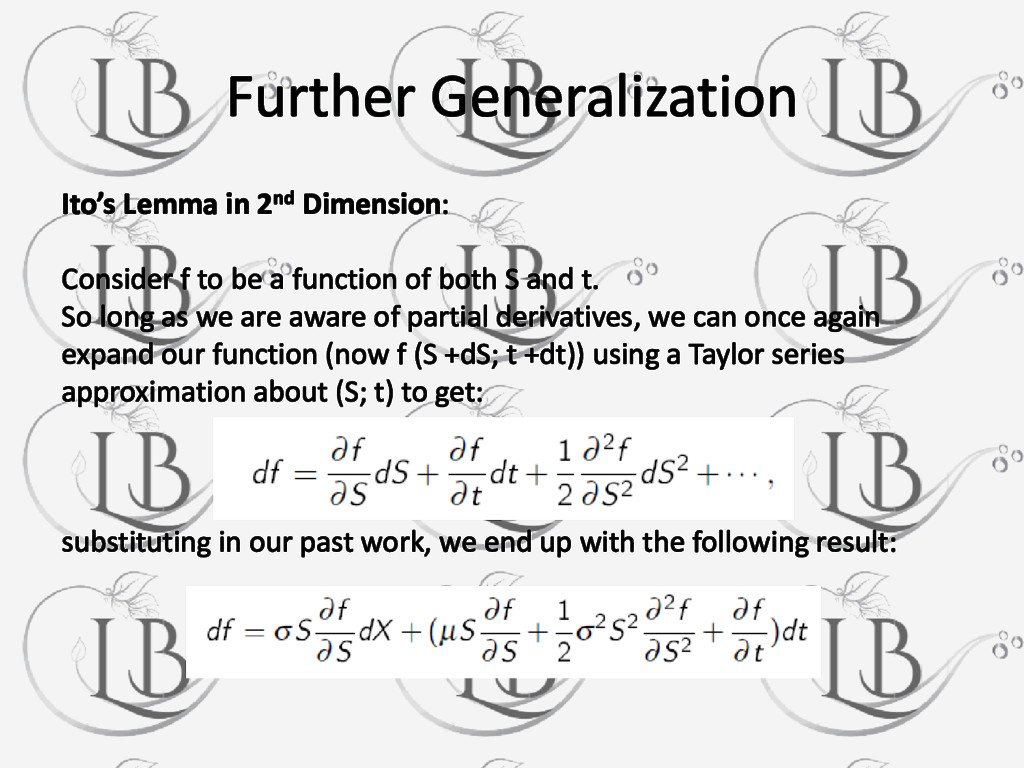
17. Further Generalization Ito’s Lemma in 2nd Dimension: Consider f to be a function of both S and t. So long as we are aware of partial derivatives, we can once again expand our function (now f (S +dS; t +dt)) using a Taylor series approximation about (S; t) to get: substituting in our past work, we end up with the following result:
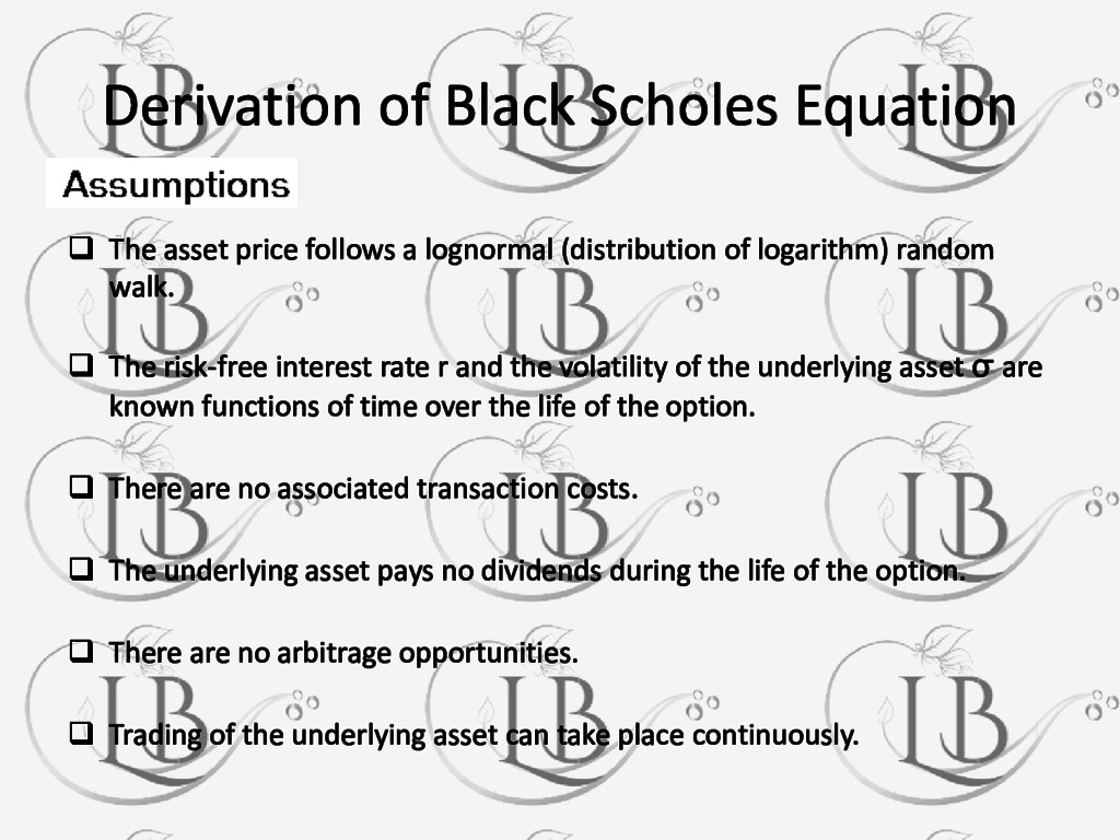
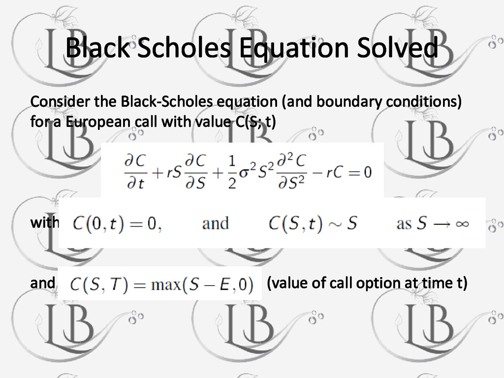
18. Derivation of Black Scholes Equation  The asset price follows a lognormal (distribution of logarithm) random walk.  The risk-free interest rate r and the volatility of the underlying asset σ are known functions of time over the life of the option.  There are no associated transaction costs.  The underlying asset pays no dividends during the life of the option.  There are no arbitrage opportunities.  Trading of the underlying asset can take place continuously.
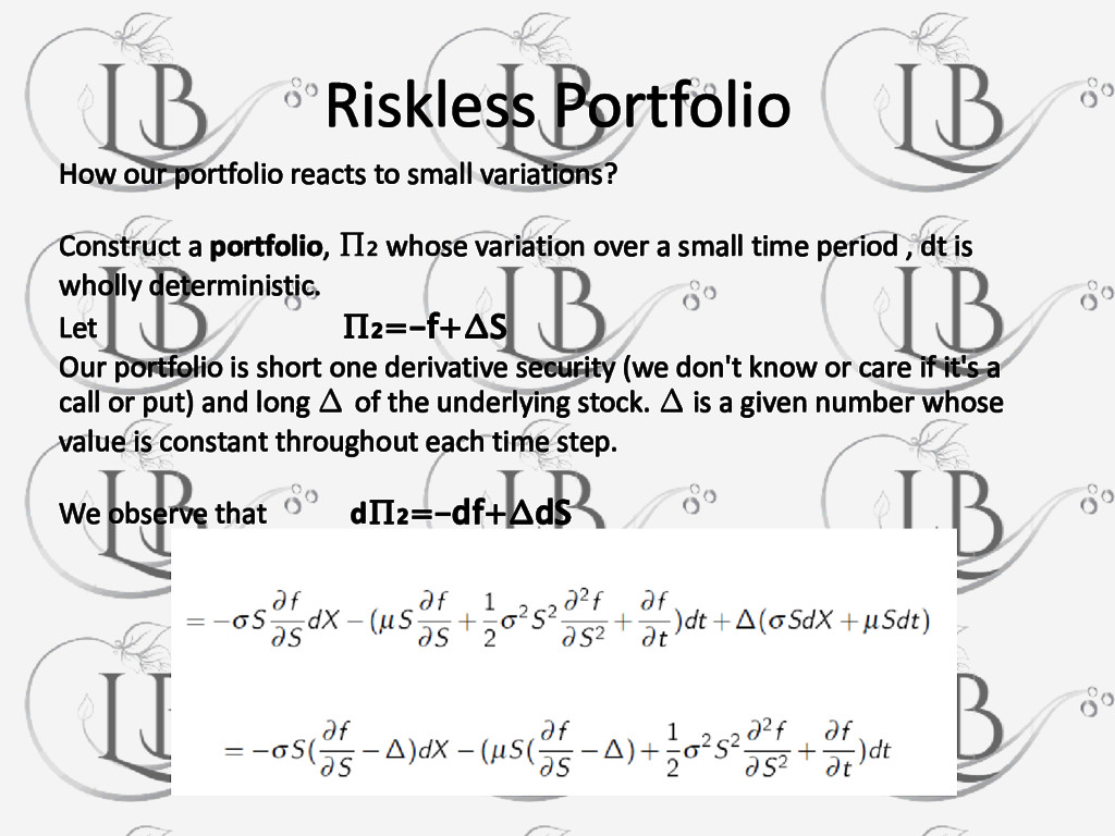
19. Riskless Portfolio How our portfolio reacts to small variations? Construct a portfolio, ∏₂ whose variation over a small time period , dt is wholly deterministic. Let ∏₂=-f+∆S Our portfolio is short one derivative security (we don't know or care if it's a call or put) and long ∆ of the underlying stock. ∆ is a given number whose value is constant throughout each time step. We observe that d∏₂=-df+∆dS
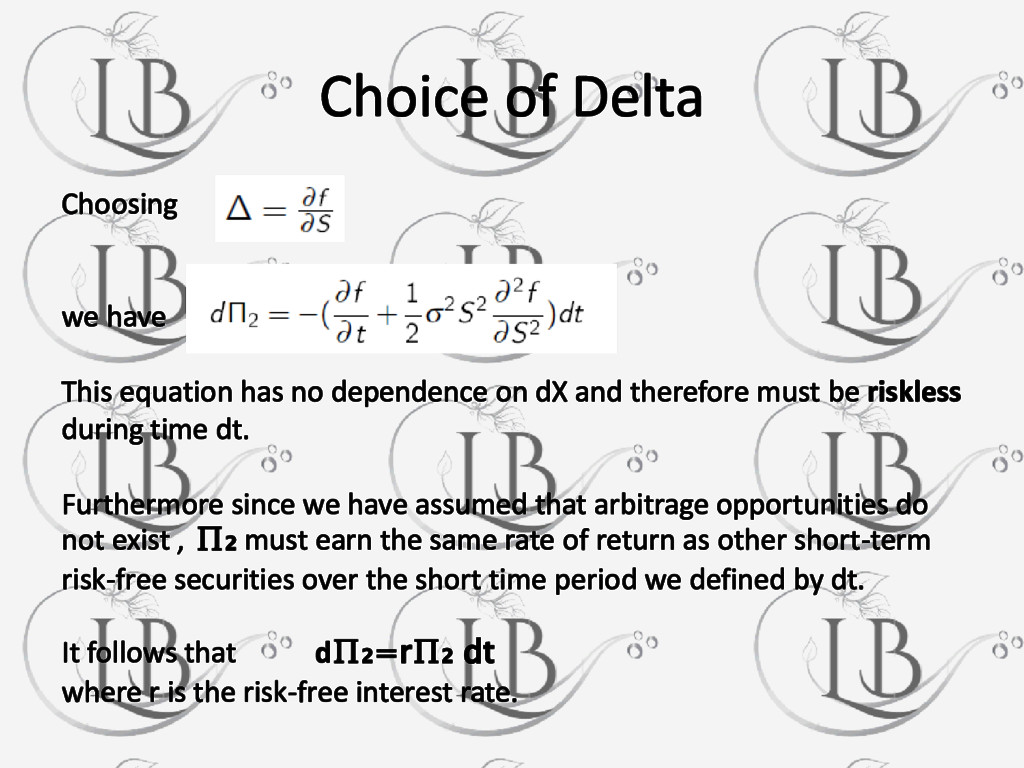
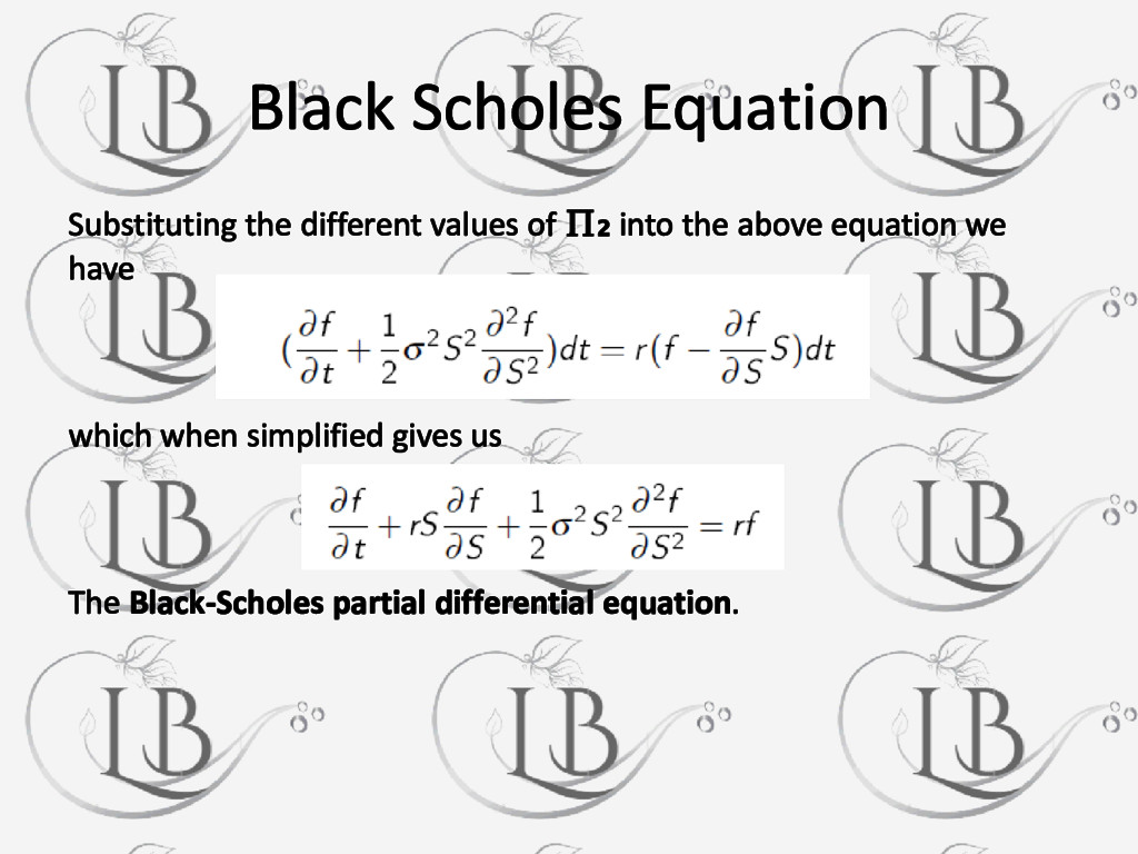
20. Choice of Delta Choosing we have This equation has no dependence on dX and therefore must be riskless during time dt. Furthermore since we have assumed that arbitrage opportunities do not exist , ∏₂ must earn the same rate of return as other short-term risk-free securities over the short time period we defined by dt. It follows that d∏₂=r∏₂ dt where r is the risk-free interest rate.
21. Black Scholes Equation Substituting the different values of ∏₂ into the above equation we have which when simplified gives us The Black-Scholes partial differential equation.
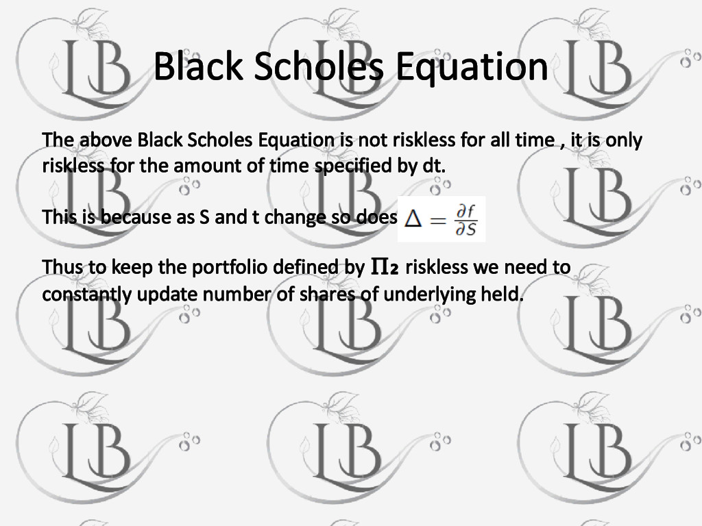
22. Black Scholes Equation The above Black Scholes Equation is not riskless for all time , it is only riskless for the amount of time specified by dt. This is because as S and t change so does Thus to keep the portfolio defined by ∏₂ riskless we need to constantly update number of shares of underlying held.
23. Black Scholes Equation Solved Consider the Black-Scholes equation (and boundary conditions) for a European call with value C(S; t) with and (value of call option at time t)
24. Substitutions We make the following substitution , to remove S & S^2 terms The above substitutions result in the following equation where and the initial condition becomes
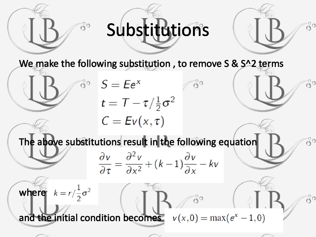
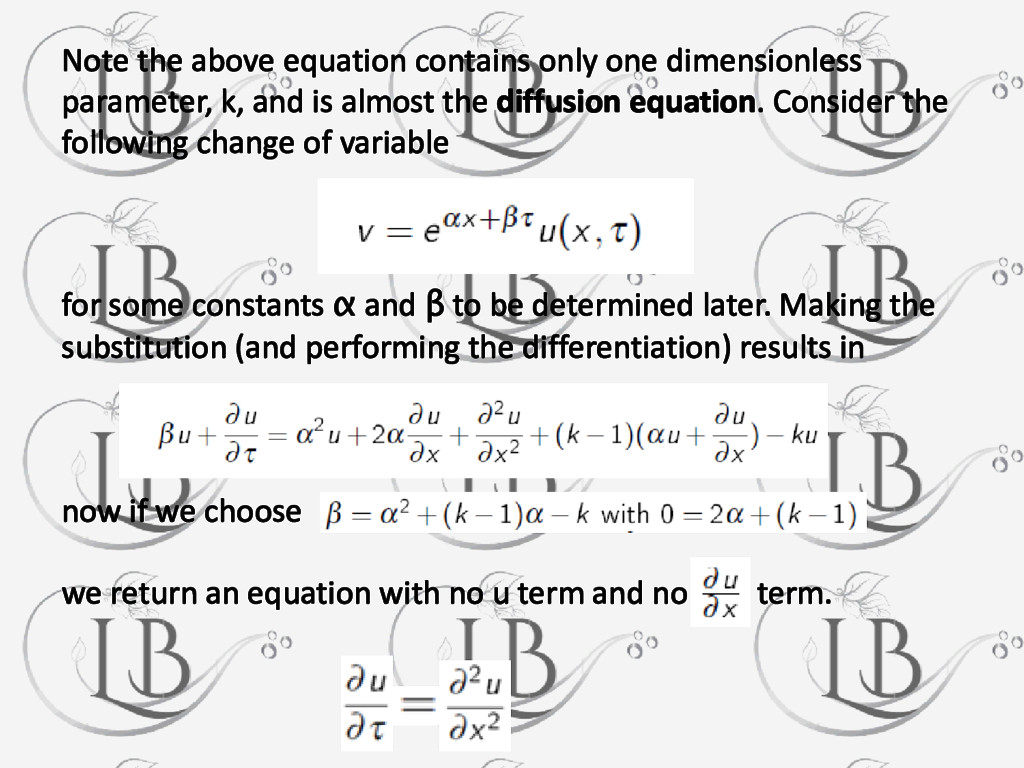
25. Note the above equation contains only one dimensionless parameter, k, and is almost the diffusion equation. Consider the following change of variable for some constants α and β to be determined later. Making the substitution (and performing the differentiation) results in now if we choose we return an equation with no u term and no term.
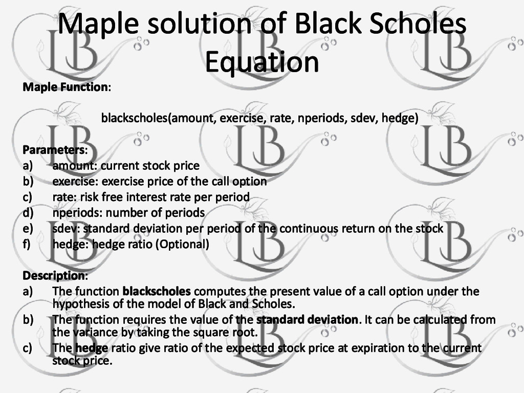
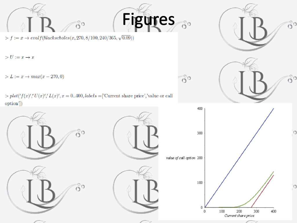
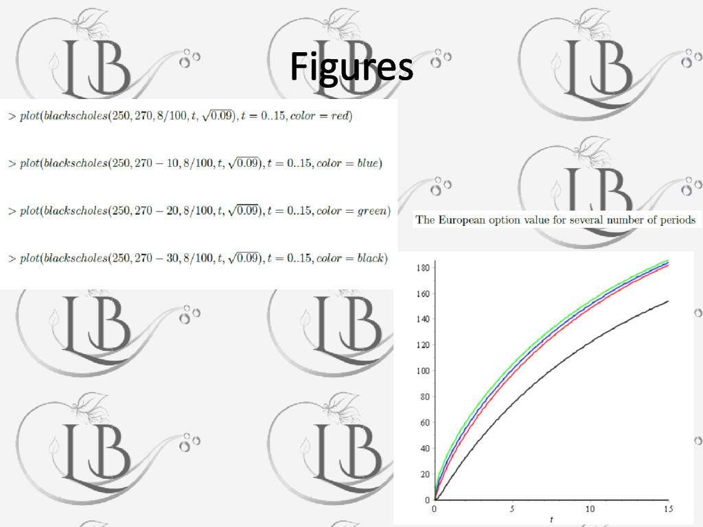
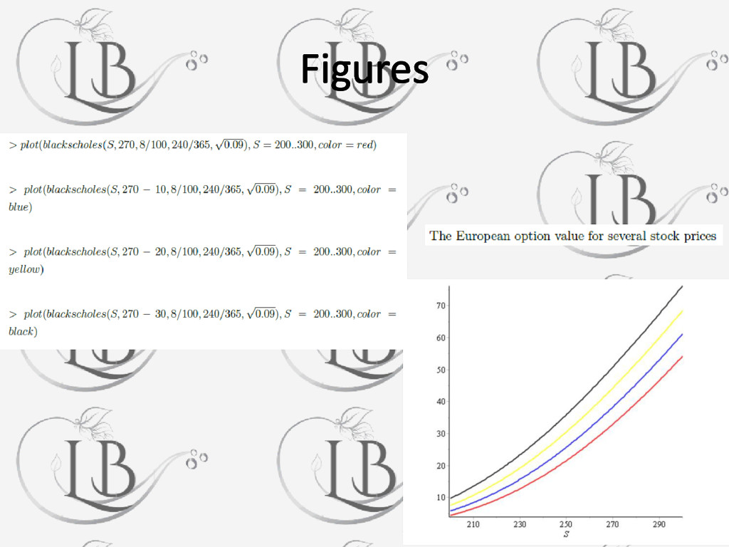
26. Maple solution of Black Scholes Equation Maple Function: blackscholes(amount, exercise, rate, nperiods, sdev, hedge) Parameters: a) amount: current stock price b) exercise: exercise price of the call option c) rate: risk free interest rate per period d) nperiods: number of periods e) sdev: standard deviation per period of the continuous return on the stock f) hedge: hedge ratio (Optional) Description: a) The function blackscholes computes the present value of a call option under the hypothesis of the model of Black and Scholes. b) The function requires the value of the standard deviation. It can be calculated from the variance by taking the square root. c) The hedge ratio give ratio of the expected stock price at expiration to the current stock price.
30. Figures
31. Figures
32. Figures
33. OPTION PRICING WITH TRANSACTION COSTS AND STOCHASTIC VOLATILITY
34. Introduction  We consider a market model in which trading the asset requires paying transaction fees which are proportional to the quantity and the value of the asset traded.  A model where the volatility is random is called Stochastic Volatility Model.  This problem is important when high-frequency data are considered. For such data, the volatility is clearly stochastic. Thus it is necessary to deal with Stochastic Volatility Model.  In this market we study the problem of finding option prices when the underlying asset may be approximated using a Stochastic Volatility Model. So basically, our main motive is to extend the transaction costs model when the asset price is approximated using stochastic volatility models.
35. Key Terms Stochastic volatility - A statistical method in mathematical finance in which volatility & co-dependence between variables is allowed to fluctuate over time rather than remain constant.  These Models for options were developed out of a need to modify Black Scholes model for option pricing , which failed to effectively take the volatility in the price of underlying security into account.  Allowing the price to vary in the Stochastic Models improved the accuracy of calculations & forecasts. Transaction Cost – Expenses incurred when buying or selling securities. These costs include broker’s commissions.  These costs to buyers and sellers are the payments that banks and brokers receive for their roles in these transactions.  These costs are important to investors because they are one of the key determinant of net return.
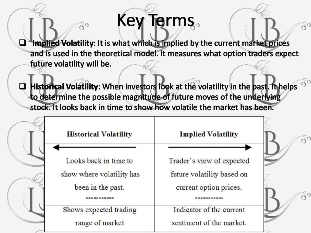
36. Key Terms  Implied Volatility: It is what which is implied by the current market prices and is used in the theoretical model. It measures what option traders expect future volatility will be.  Historical Volatility: When investors look at the volatility in the past. It helps to determine the possible magnitude of future moves of the underlying stock. It looks back in time to show how volatile the market has been.
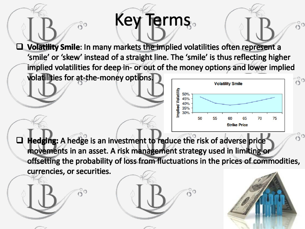
37. Key Terms  Volatility Smile: In many markets the implied volatilities often represent a ‘smile’ or ‘skew’ instead of a straight line. The ‘smile’ is thus reflecting higher implied volatilities for deep in- or out of the money options and lower implied volatilities for at-the-money options.  Hedging: A hedge is an investment to reduce the risk of adverse price movements in an asset. A risk management strategy used in limiting or offsetting the probability of loss from fluctuations in the prices of commodities, currencies, or securities.
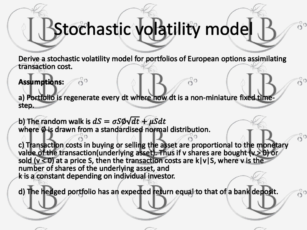
38. Stochastic volatility model Derive a stochastic volatility model for portfolios of European options assimilating transaction cost. Assumptions: a) Portfolio is regenerate every dt where now dt is a non-miniature fixed time- step. b) The random walk is = ∅ + where ∅ is drawn from a standardised normal distribution. c) Transaction costs in buying or selling the asset are proportional to the monetary value of the transaction(underlying asset). Thus if v shares are bought (v > 0) or sold (v < 0) at a price S, then the transaction costs are k|v|S, where v is the number of shares of the underlying asset, and k is a constant depending on individual investor. d) The hedged portfolio has an expected return equal to that of a bank deposit.
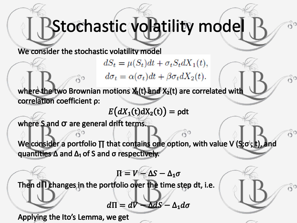
39. Stochastic volatility model We consider the stochastic volatility model where the two Brownian motions X₁(t) and X₂(t) are correlated with correlation coefficient ρ: ₁ t dX₂ t = ρdt where S and σ are general drift terms. We consider a portfolio ∏ that contains one option, with value V (S;σ ; t), and quantities ∆ and ∆₁ of S and σ respectively. Π = − ∆ − ∆₁ Then dП changes in the portfolio over the time step dt, i.e. Π = − ∆ − ∆₁ Applying the Ito’s Lemma, we get
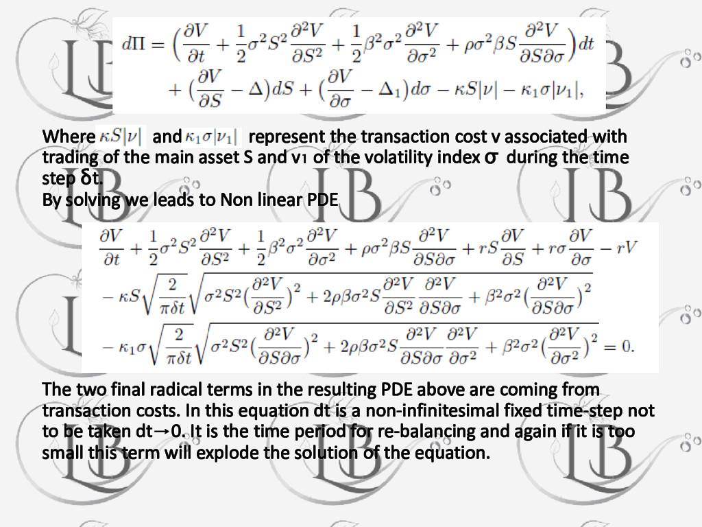
40. Where and represent the transaction cost v associated with trading of the main asset S and v₁ of the volatility index σ during the time step δt. By solving we leads to Non linear PDE The two final radical terms in the resulting PDE above are coming from transaction costs. In this equation dt is a non-infinitesimal fixed time-step not to be taken dt→0. It is the time period for re-balancing and again if it is too small this term will explode the solution of the equation.
41. Quanto Option Pricing Model
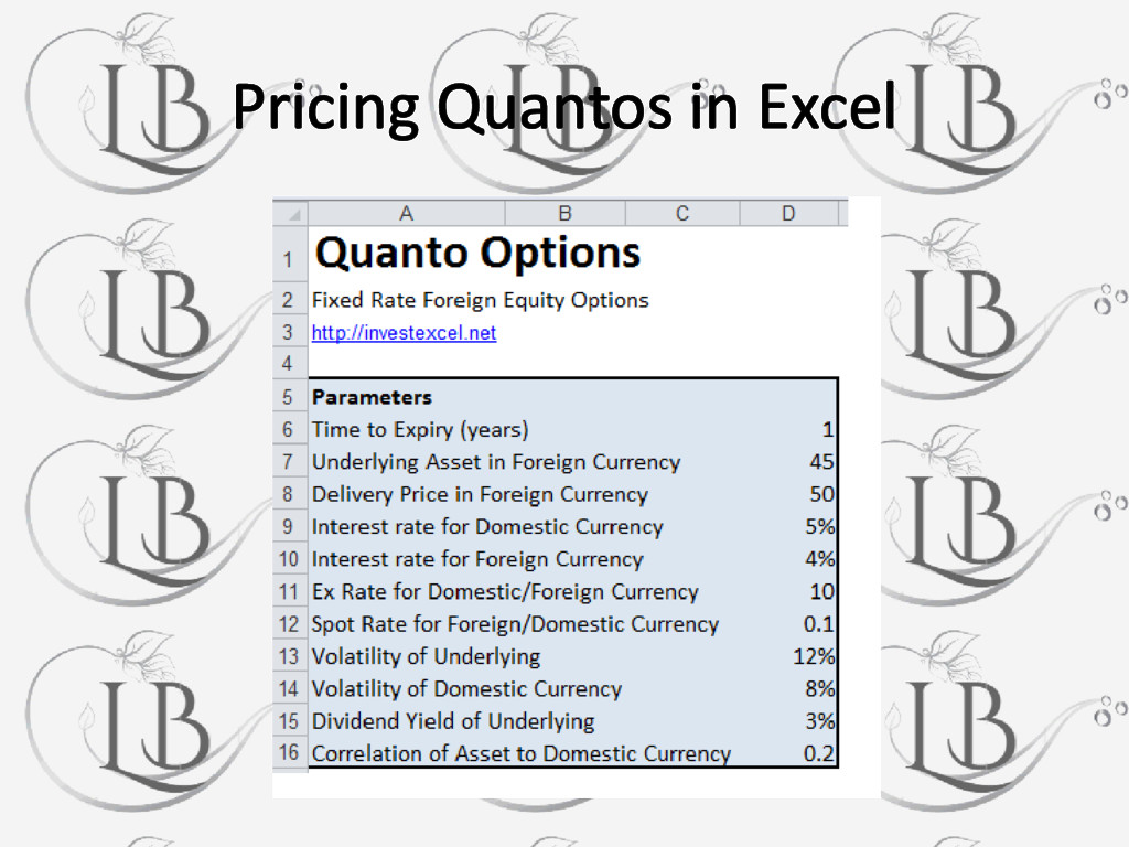
42. Key Terms Quanto: It is a type of derivative in which the underlying is denominated in one currency, but the instrument itself is settled in another currency at some rate. Quantos are attractive because they shield the purchaser from exchange rate fluctuations. The name “quanto” is, in fact, derived from the variable notional amount, and is short for “quantity adjusting option”. Quanto options: A cash-settled, cross-currency derivative in which the underlying asset is denominated in a currency other than the currency in which the option is settled. Quantos are settled at a fixed rate of exchange, providing investors with shelter from exchange-rate risk. At the time of expiration, the option's value is calculated in the amount of foreign currency and then converted at a fixed rate into the domestic currency. Basically, options in which the difference between the underlying and a fixed strike price is paid out in another currency.
43. Pricing Quantos in Excel
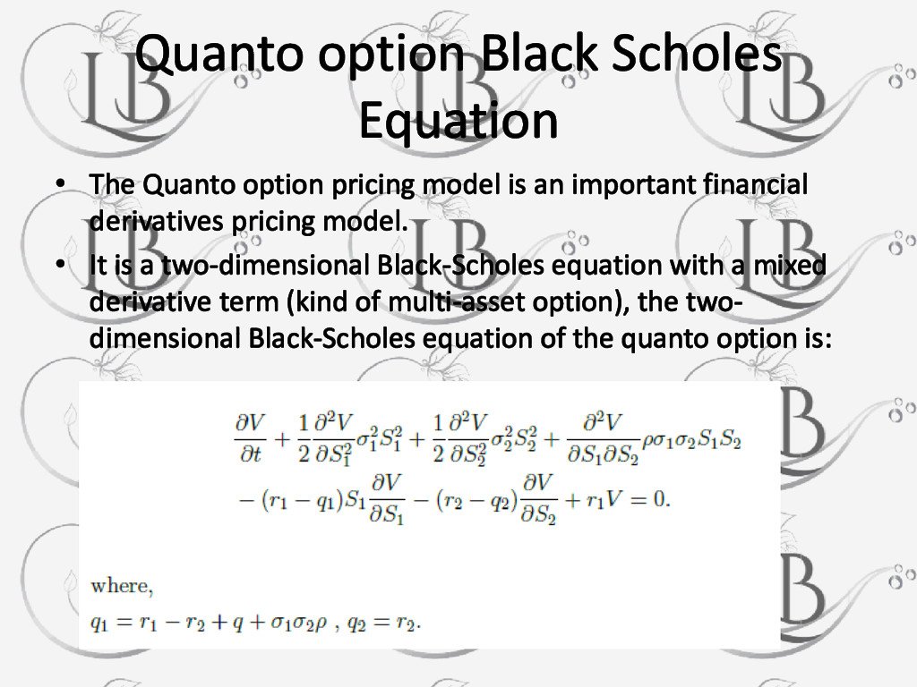
44. Quanto option Black Scholes Equation • The Quanto option pricing model is an important financial derivatives pricing model. • It is a two-dimensional Black-Scholes equation with a mixed derivative term (kind of multi-asset option), the two- dimensional Black-Scholes equation of the quanto option is:
45. Quanto option Black Scholes Equation We have assumed that an American investor buys a Nikkei index call option. Assumptions:
46. Quanto option Black Scholes Equation Solved The Analytical Solution of 2D Black-Scholes equation of the Quanto options is: is the strike price of the option (yen), and is the due date of the options (year).
47. References ▪ P.Witmott, S.Howison, and J.Dewynne; The mathematics of financial derivative, Cambridge University press, USA, 1995. ▪ M. C. Mariani, I. SenGupta, and G.Sewell; Numerical methods applied to option pricing models with transaction costs and stochastic volatility, Quantitative Finance, 2015, Vol. 15, No. 8, 1417- 1424. ▪ X.Yang, L.Wu, and Y.Shi; A new kind of parallel nite dierence methods for the quanto option pricing model, Yang et al. Advances in Differential Equations (2015) 2015:311. ▪ http://www.investopedia.com/terms/b/blackscholes.asp?optm=orig ▪ http://www.investopedia.com/video/play/blackscholes-model/ ▪ https://en.wikipedia.org/wiki/Black%E2%80%93Scholes_model#cite_note-div_yield-3 ▪ http://worldmarketpulse.com/Investing/Options/Advantages-And-Limitations-Of-Black-Scholes- Model.html ▪ https://en.wikipedia.org/wiki/BlackScholes_model#Short_stock_rate ▪ http://www.diva-portal.org/smash/get/diva2:121095/FULLTEXT01.pdf ▪ http://investexcel.net/wp-content/uploads/2012/02/Quanto-Options.png