stan推定後の可視化について Tokyo.R#94

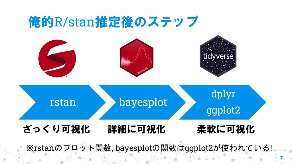
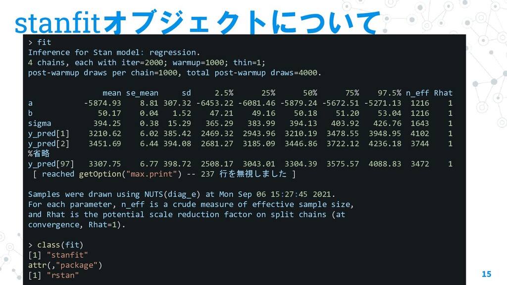
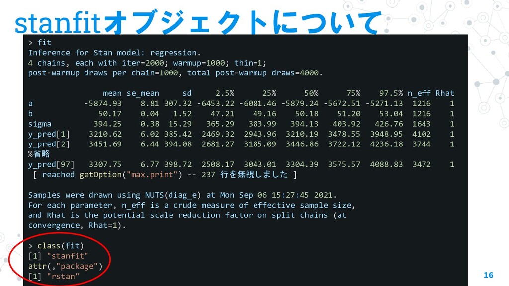
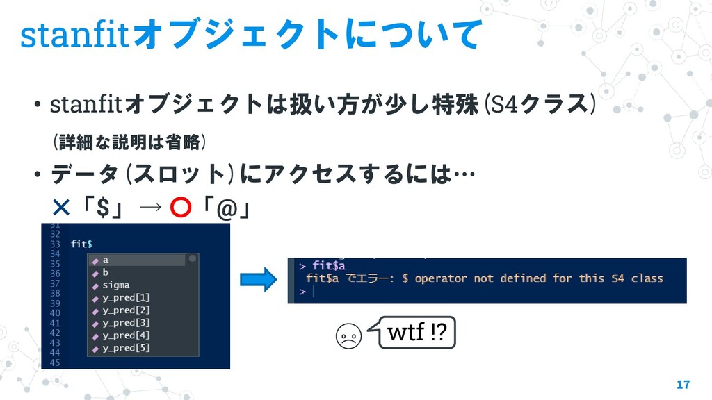
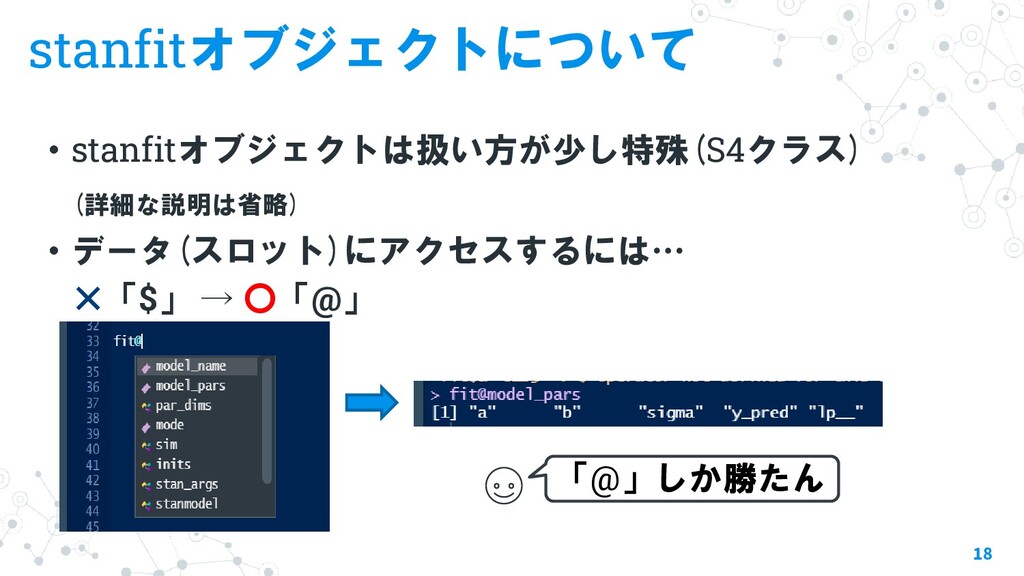
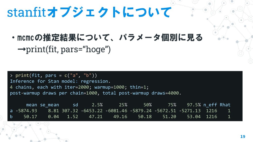
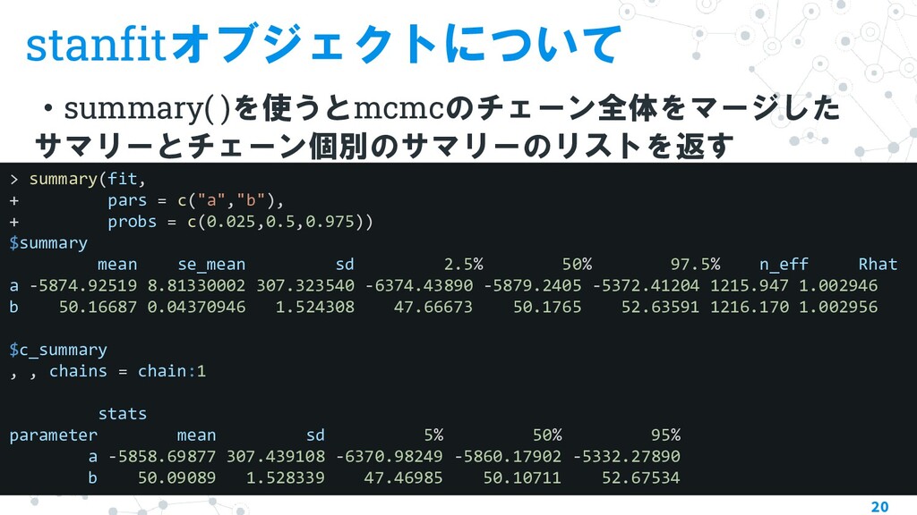
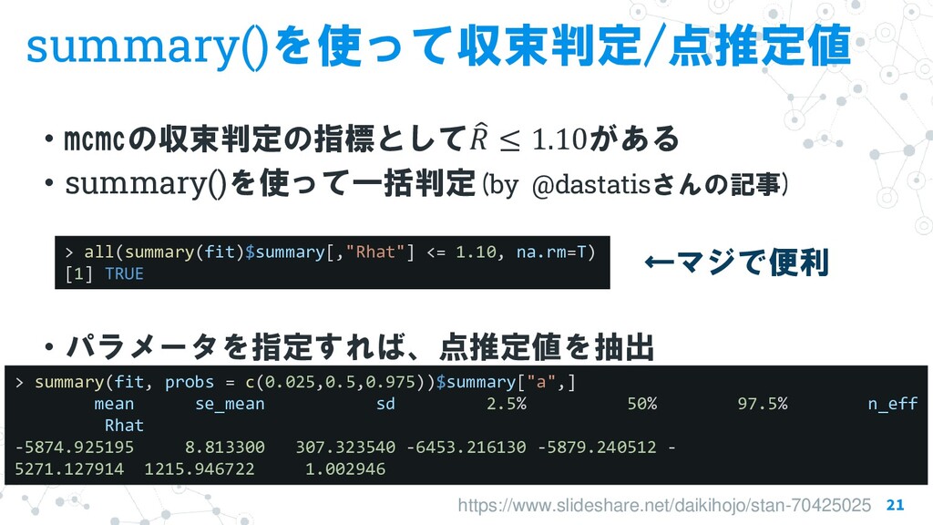
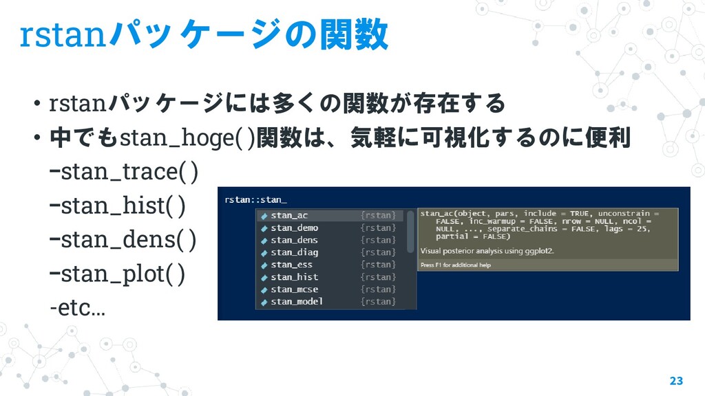
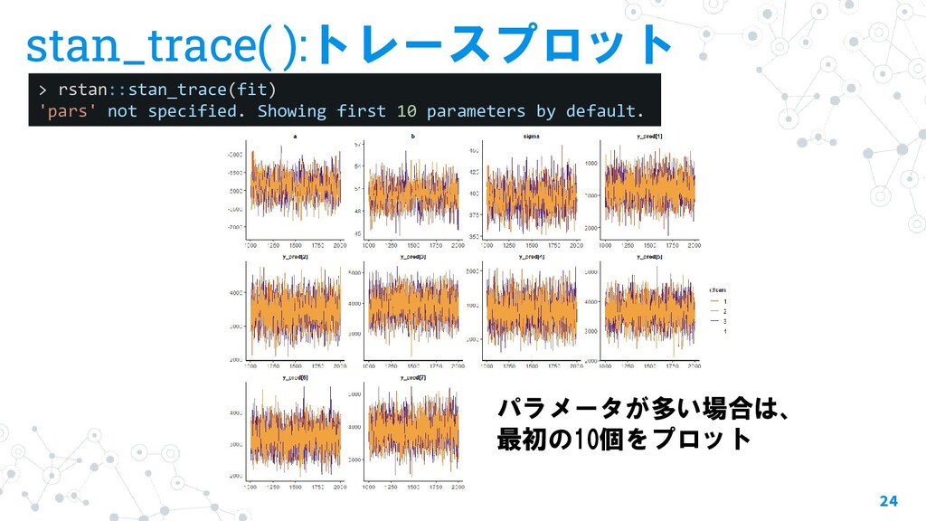
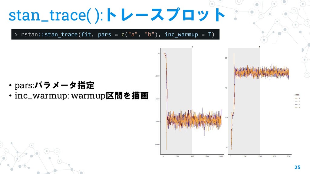
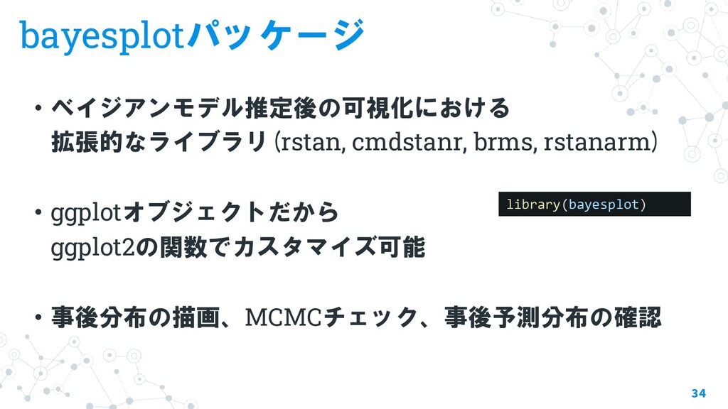
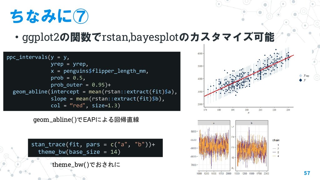
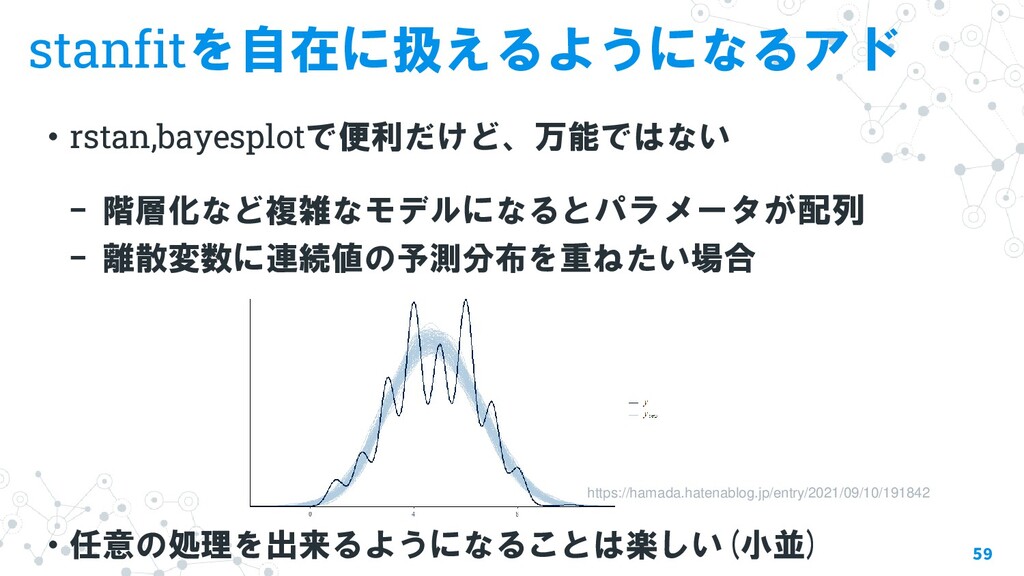
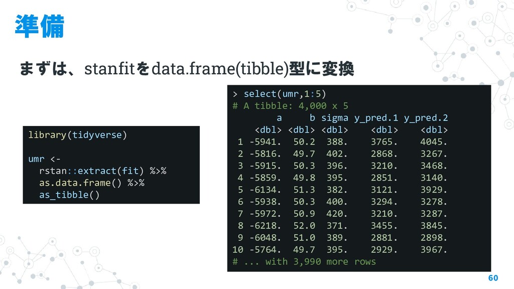
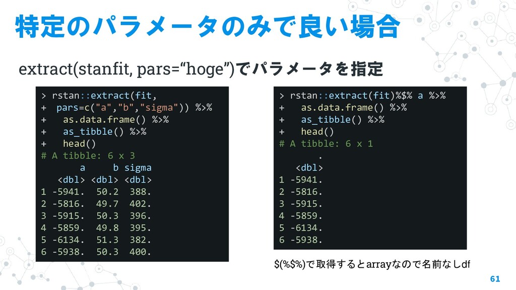
stan推定後の可視化に便利なパッケージとその関数について紹介します。
・stanfitオブジェクトについて
・rstanパッケージの関数
・bayesplotパッケージの関数
・tidyverseでstanfitを扱う

1. stan推定後の可視化について Tokyo.R#94 (2021/09/11) by ando_Roid @hirahira2835
2. 自己紹介 名前: 安藤正和 ・専攻: 心理学(M2) ・R/stan歴: 3年 ・ベイズ統計なんもわからん 2
3. 3 https://qiita.com/ando_roid/items/d37028ea65953a1e53d9 https://qiita.com/ando_roid/items/8e7142f8c87e5e0f44b0
4. stanは、本はもちろん日本語の神記事いっぱい 4 https://das-kino.hatenablog.com/entry/2018/12/10/211511 https://ill-identified.hatenablog.com/entry/2019/06/13/010510 https://www.slideshare.net/daikihojo/stan-70425025
5. stan推定後にやりたいこと ・MCMCの収束判定 ・パラメータの挙動確認 ・事後予測分布/予測値の確認 etc… 5
6. 俺的R/stan推定後のステップ 6 rstan bayesplot dplyr ggplot2 ざっくり可視化 詳細に可視化 柔軟に可視化
7. 俺的R/stan推定後のステップ 7 rstan bayesplot dplyr ggplot2 ざっくり可視化 詳細に可視化 柔軟に可視化 ※rstanのプロット関数, bayesplotの関数はggplot2が使われている!
8. 目次 ◎ stanfitオブジェクトについて ◎ rstanパッケージの関数 ◎ beyesplotパッケージの関数 ◎ tidyverseでstanfitを扱う 8
9. 準備 ・今回はpalmerpenguinsパッケージのデータを使う ・penguinsには、3種類334匹のペンギンちゃん ・変数(8つ) -species: 種類 -island: 生息地(島) -bill_length_mm: くちばしの長さ -bill_depth_mm: くちばしの高さ(?) -flipper_length_mm: 翼の長さ -etc… 9 https://allisonhorst.github.io/palmerpenguins/
10. penguinsデータ 10 > install.packages("palmerpenguins") > library(palmerpenguins) > Penguins # A tibble: 333 x 8 species island bill_length_mm bill_depth_mm flipper_length_mm body_mass_g sex year <fct> <fct> <dbl> <dbl> <int> <int> <fct> <int> 1 Adelie Torgersen 39.1 18.7 181 3750 male 2007 2 Adelie Torgersen 39.5 17.4 186 3800 female 2007 3 Adelie Torgersen 40.3 18 195 3250 female 2007 4 Adelie Torgersen 36.7 19.3 193 3450 female 2007 5 Adelie Torgersen 39.3 20.6 190 3650 male 2007 6 Adelie Torgersen 38.9 17.8 181 3625 female 2007 7 Adelie Torgersen 39.2 19.6 195 4675 male 2007 8 Adelie Torgersen 41.1 17.6 182 3200 female 2007 9 Adelie Torgersen 38.6 21.2 191 3800 male 2007 10 Adelie Torgersen 34.6 21.1 198 4400 male 2007 # ... with 323 more rows
11. 準備 ・単回帰モデル -従属変数: body_mass_g(ペンギンの体重) -独立変数: flipper_length_mm(ペンギンの翼の長さ) 11 library(tidyverse) penguins %>% ggplot()+ aes(x=flipper_length_mm, body_mass_g)+ geom_point()+ geom_smooth(formula = "y~x", method = "lm",se=F)+ theme_bw(base_size = 14)
12. stanコード 12 data{ int N; vector[N] Y; vector[N] X; } parameters{ real a; //切片 real b; //flipper_length_mmの係数項 real<lower = 0> sigma; //標準偏差 } model{ Y ~ normal(a + b*X, sigma); } generated quantities{ vector[N] y_pred; //事後予測分布みるための生成量 for(n in 1:N){ y_pred[n] = normal_rng(a + b*X[n], sigma); } } ・regression.stan として保存
13. Rコード 13 library(rstan) library(magrittr) # 性別のNAを除去 penguins %<>% filter(!is.na(sex)) stanmodel <- rstan::stan_model("regression.stan") standata <- list(N = nrow(penguins), Y = penguins$body_mass_g, X = penguins$flipper_length_mm) fit <- rstan::sampling(object = stanmodel, data = standata, seed = 42, iter = 2000, warmup = 1000, chain = 4) ・性別のNAを除去 ・推定結果をfitに格納 ・mcmcの設定 - iter=2000 - warmup=1000 - chain=4 - 計4000サンプル
14. stanfitオブジェクトについて
15. stanfitオブジェクトについて 15 > fit Inference for Stan model: regression. 4 chains, each with iter=2000; warmup=1000; thin=1; post-warmup draws per chain=1000, total post-warmup draws=4000. mean se_mean sd 2.5% 25% 50% 75% 97.5% n_eff Rhat a -5874.93 8.81 307.32 -6453.22 -6081.46 -5879.24 -5672.51 -5271.13 1216 1 b 50.17 0.04 1.52 47.21 49.16 50.18 51.20 53.04 1216 1 sigma 394.25 0.38 15.29 365.29 383.99 394.13 403.92 426.76 1643 1 y_pred[1] 3210.62 6.02 385.42 2469.32 2943.96 3210.19 3478.55 3948.95 4102 1 y_pred[2] 3451.69 6.44 394.08 2681.27 3185.09 3446.86 3722.12 4236.18 3744 1 %省略 y_pred[97] 3307.75 6.77 398.72 2508.17 3043.01 3304.39 3575.57 4088.83 3472 1 [ reached getOption("max.print") -- 237 行を無視しました ] Samples were drawn using NUTS(diag_e) at Mon Sep 06 15:27:45 2021. For each parameter, n_eff is a crude measure of effective sample size, and Rhat is the potential scale reduction factor on split chains (at convergence, Rhat=1). > class(fit) [1] "stanfit" attr(,"package") [1] "rstan"
16. stanfitオブジェクトについて 16 > fit Inference for Stan model: regression. 4 chains, each with iter=2000; warmup=1000; thin=1; post-warmup draws per chain=1000, total post-warmup draws=4000. mean se_mean sd 2.5% 25% 50% 75% 97.5% n_eff Rhat a -5874.93 8.81 307.32 -6453.22 -6081.46 -5879.24 -5672.51 -5271.13 1216 1 b 50.17 0.04 1.52 47.21 49.16 50.18 51.20 53.04 1216 1 sigma 394.25 0.38 15.29 365.29 383.99 394.13 403.92 426.76 1643 1 y_pred[1] 3210.62 6.02 385.42 2469.32 2943.96 3210.19 3478.55 3948.95 4102 1 y_pred[2] 3451.69 6.44 394.08 2681.27 3185.09 3446.86 3722.12 4236.18 3744 1 %省略 y_pred[97] 3307.75 6.77 398.72 2508.17 3043.01 3304.39 3575.57 4088.83 3472 1 [ reached getOption("max.print") -- 237 行を無視しました ] Samples were drawn using NUTS(diag_e) at Mon Sep 06 15:27:45 2021. For each parameter, n_eff is a crude measure of effective sample size, and Rhat is the potential scale reduction factor on split chains (at convergence, Rhat=1). > class(fit) [1] "stanfit" attr(,"package") [1] "rstan"
17. stanfitオブジェクトについて ・stanfitオブジェクトは扱い方が少し特殊(S4クラス) (詳細な説明は省略) ・データ(スロット)にアクセスするには… ×「$」 → 〇「@」 17 wtf !?
18. stanfitオブジェクトについて 18 「@」しか勝たん ・stanfitオブジェクトは扱い方が少し特殊(S4クラス) (詳細な説明は省略) ・データ(スロット)にアクセスするには… ×「$」 → 〇「@」
19. stanfitオブジェクトについて ・mcmcの推定結果について、パラメータ個別に見る →print(fit, pars=“hoge”) 19 > print(fit, pars = c("a", "b")) Inference for Stan model: regression. 4 chains, each with iter=2000; warmup=1000; thin=1; post-warmup draws per chain=1000, total post-warmup draws=4000. mean se_mean sd 2.5% 25% 50% 75% 97.5% n_eff Rhat a -5874.93 8.81 307.32 -6453.22 -6081.46 -5879.24 -5672.51 -5271.13 1216 1 b 50.17 0.04 1.52 47.21 49.16 50.18 51.20 53.04 1216 1
20. stanfitオブジェクトについて ・summary( )を使うとmcmcのチェーン全体をマージした サマリーとチェーン個別のサマリーのリストを返す 20 > summary(fit, + pars = c("a","b"), + probs = c(0.025,0.5,0.975)) $summary mean se_mean sd 2.5% 50% 97.5% n_eff Rhat a -5874.92519 8.81330002 307.323540 -6374.43890 -5879.2405 -5372.41204 1215.947 1.002946 b 50.16687 0.04370946 1.524308 47.66673 50.1765 52.63591 1216.170 1.002956 $c_summary , , chains = chain:1 stats parameter mean sd 5% 50% 95% a -5858.69877 307.439108 -6370.98249 -5860.17902 -5332.27890 b 50.09089 1.528339 47.46985 50.10711 52.67534
21. summary()を使って収束判定/点推定値 ・mcmcの収束判定の指標として ෠ 𝑅 ≤ 1.10がある ・summary()を使って一括判定(by @dastatisさんの記事) ・パラメータを指定すれば、点推定値を抽出 21 > all(summary(fit)$summary[,"Rhat"] <= 1.10, na.rm=T) [1] TRUE https://www.slideshare.net/daikihojo/stan-70425025 > summary(fit, probs = c(0.025,0.5,0.975))$summary["a",] mean se_mean sd 2.5% 50% 97.5% n_eff Rhat -5874.925195 8.813300 307.323540 -6453.216130 -5879.240512 - 5271.127914 1215.946722 1.002946 ←マジで便利
22. rstanパッケージの関数
23. rstanパッケージの関数 ・rstanパッケージには多くの関数が存在する ・中でもstan_hoge( )関数は、気軽に可視化するのに便利 -stan_trace( ) -stan_hist( ) -stan_dens( ) -stan_plot( ) -etc… 23
24. stan_trace( ):トレースプロット 24 > rstan::stan_trace(fit) 'pars' not specified. Showing first 10 parameters by default. パラメータが多い場合は、 最初の10個をプロット
25. stan_trace( ):トレースプロット 25 > rstan::stan_trace(fit, pars = c("a", "b"), inc_warmup = T) ・pars:パラメータ指定 ・inc_warmup: warmup区間を描画
26. 上手く推定できていない時… 26 https://discourse.mc-stan.org/t/gaussian-process-on-hpc-issues-and-speeding-up/18202 [mcmcあるある] ・あるチェインだけ変な挙動 ・局所解 ※色んなトレースプロットを集めよう(?)
27. stan_dens( ): デンシティプロット 27 > rstan::stan_dens(fit, pars = c("a", "b")) > rstan::stan_dens(fit, pars = c("a", "b"), separate_chains = T) ・separate_chains: チェイン別に描画するかどうか separate_chains = FALSE separate_chains = TRUE
28. 上手く推定できていない時 28 http://www.eeso.ges.kyoto-u.ac.jp/emm/materials/bayesian/stan_step1 [mcmcあるある] ・多峰性 ・チェインでばらばら ※色んなデンシティプロットを集めよう(?)
29. stan_hist( ): ヒストグラム 29 rstan::stan_hist(fit, pars = c("a", "b"), bins=40) ・bins: 数値の幅を調整
30. stan_ac( ): 自己相関 30 rstan::stan_ac(fit, pars = c("a", "b")) 効率よくサンプリングが行われている場合、自己相関はすぐに減少 引数 ・lags: 描画する最大のlag数 ・separate_chains ・inc_warmup
31. stan_rhat( ): ෠ 𝑅のプロット 31 rstan::stan_rhat(fit) 推定したパラメータ、生成量の ෠ 𝑅を確認 → 全ての ෠ 𝑅 ≤ 1.10 ※chain=1では無理
32. stan_plot( ):事後分布の区間と点推定値 32 rstan::stan_plot(fit, point_est ="mean", show_density = T, ci_level = 0.8, outer_level = 1) 引数 ・point_est:点推定値の代表値 ・show_density:分布の山の表示 ・ci_level:確信区間の範囲 ・outer_level:分布どこまで表示するか ・fill_color, outline_color, est_colorでそれぞれの色をカスタマイズできるお
33. bayesplotパッケージの関数
34. bayesplotパッケージ ・ベイジアンモデル推定後の可視化における 拡張的なライブラリ(rstan, cmdstanr, brms, rstanarm) ・ggplotオブジェクトだから ggplot2の関数でカスタマイズ可能 ・事後分布の描画、MCMCチェック、事後予測分布の確認 34 library(bayesplot)
35. bayesplotパッケージの関数 ・mcmc_hoge( ): MCMCの描画/診断系関数 ・ppc_hoge( ): 事後予測チェック系関数 ppc…posterior predictive check 35
36. mcmc_hoge()系
37. mcmc_trace( ): トレースプロット 37 mcmc_trace(fit, pars = c("a", "b")) mcmc_trace_highlight(fit, pars = c("a", "b"), highlight = 1) #チェイン 特定のチェインとそれ以外のチェインの挙動の比較
38. ちなみに① ・bayesplotのプロット関数(mcmc_trace()など)は、 parsを指定しないと、全パラメータを描画する 38 mcmc_trace(fit)
39. mcmc_rhat(rhat ): ෠ 𝑅のプロット 39 mcmc_rhat(rhat(fit)) > all(rhat(fit) <= 1.10, na.rm = T) [1] TRUE 描画しなくても(ry rhat( )はパラメータの ෠ 𝑅をベクトルで返す mcmc_rhat(rhat(fit,pars=c("a","b","sigma")))+ yaxis_text(hjust=1) パラメータ指定して、y軸にパラメータ名
40. mcmc_dens( ): デンシティプロット 40 mcmc_dens(fit, pars = c("a", "b")) mcmc_dens_overlay(fit, pars = c("a", "b"))
41. mcmc_hist( ): ヒストグラム 41 mcmc_hist(fit, pars = c("a", "b")) mcmc_hist_by_chain(fit, pars = c("a", "b"))
42. ちなみに② 大抵のmcmc_hoge( )内でパラメータの変換可能(transformations) 42 mcmc_hist(fit, pars = "sigma", transformations = list(sigma = "log"))
43. mcmc_scatter( ):二変数の散布図 43 mcmc_scatter(fit, pars = c("a", "b")) mcmc_hex(fit, pars = c("a", "b")) ※hexbinパッケージが必要 事後サンプルサイズが大きいときに有効 sizeやalphaの変更可能
44. mcmc_pairs( ): 1・2変量の事後分布 44 mcmc_pairs(fit, pars = c("a","b","sigma")) chain:1~2 chain:3~4
45. ちなみに③ ・気分に合わせてプロット時の配色を変更可能 45 color_scheme_set("darkgray") color_scheme_set(“teal") color_scheme_set("brewer-Spectral") mcmc_trace(fit, pars = "sigma") https://mc-stan.org/bayesplot/reference/bayesplot-colors.html
46. ppc_hoge()系
47. ppc_hoge()系 ・事後予測チェック(posterior predictive check) 系関数 ・ppc_hoge(y, yrep)は基本的に二つの引数を取る - y: 従属変数 - yrep: 事後予測分布から複製(replicate)されたサンプル (generated quantitiesブロックで生成した乱数) 47
48. 準備 ・MCMCの結果は rstan::extract( )で取得可能 ・dollar演算子(%$%)でも取得可能(library(magrittr)) ・rstan::extract(fit,pars=)だとリスト型 48 > y <- penguins$body_mass_g > yrep <- rstan::extract(fit)$y_pred > class(yrep) [1] "matrix" > rstan::extract(fit) %$% yrep %>% class() [1] "matrix" > class(rstan::extract(fit,pars="y_pred")) [1] "list"
49. ちなみに④ 49 > extract(fit) Error in UseMethod("extract_") : no applicable method for 'extract_' applied to an object of class "stanfit" ・extract()はconflictしやすいのでrstan::を付けることを推奨 wtf !? > rstan::extract(fit) 「rstan::」しか勝たん
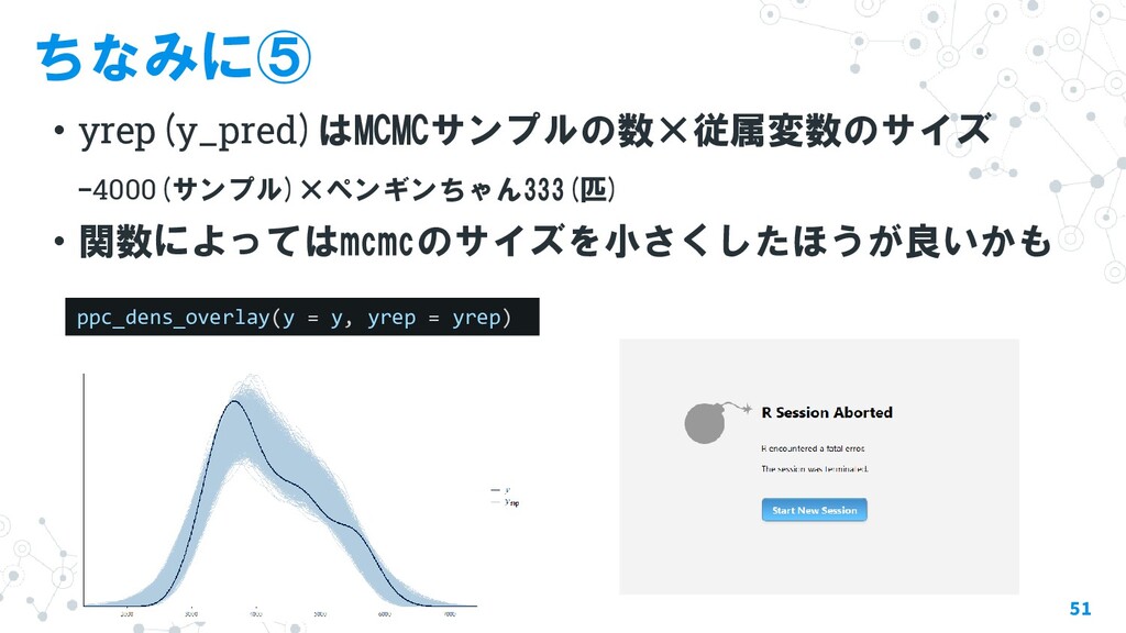
50. ppc_dens_overlay( ):データと予測値の密度分布比較 50 ppc_dens_overlay(y = y, yrep = yrep[sample(nrow(yrep), 10),]) ・濃線: 従属変数のデータ ・薄線: 事後予測分布からのmcmcサンプル yrep[sample(nrow(yrep), 10),] →ランダムにmcmcサンプルから 10セットとってくる
51. ちなみに⑤ ・yrep(y_pred)はMCMCサンプルの数×従属変数のサイズ -4000(サンプル)×ペンギンちゃん333(匹) ・関数によってはmcmcのサイズを小さくしたほうが良いかも 51 ppc_dens_overlay(y = y, yrep = yrep)
52. ppc_hist( ), ppc_boxplot( ) ・ヒストグラムやボックスプロットでの比較 52 ppc_hist(y, yrep[sample(nrow(yrep), 5),]) ppc_boxplot(y, yrep[sample(nrow(yrep), 5),])
53. ちなみに⑥ ・ppc_hoge_grouped(y,yrep,group) ・グループごとに事後予測チェックできる関数もある 53 https://mc-stan.org/bayesplot/reference/PPC-distributions.html ppc_violin_grouped(y, yrep, group, size = 1.5) ppc_dens_grouped(y, yrep, group, size = 1.5)
54. ppc_error_hoge( ): 予測誤差のプロット データと予測値の誤差(y - yrep)をヒストグラムや散布図で可視化 54 ppc_error_hist(y, yrep[sample(nrow(yrep), 3),])+ yaxis_text() ppc_error_scatter(y, yrep[sample(nrow(yrep), 4),])
55. ppc interval: 独立変数との関連も見る ・ppc_ribbon( ): 独立変数が従属変数に及ぼす影響をリボン表示 55 ppc_ribbon(y = y, yrep = yrep, x = penguins$flipper_length_mm, prob = 0.5, prob_outer = 0.95) ・prob, prob:_outer: 表示する区間幅
56. ppc interval: 独立変数との関連も見る ・ppc_intervals( ): 独立変数が従属変数に及ぼす影響を点と区間表示 56 ppc_intervals(y = y, yrep = yrep, x = penguins$flipper_length_mm, prob = 0.5, prob_outer = 0.95) サンプルサイズが大きいと分かりづらいかも…?
57. ちなみに⑦ ・ggplot2の関数でrstan,bayesplotのカスタマイズ可能 57 ppc_intervals(y = y, yrep = yrep, x = penguins$flipper_length_mm, prob = 0.5, prob_outer = 0.95)+ geom_abline(intercept = mean(rstan::extract(fit)$a), slope = mean(rstan::extract(fit)$b), col = “red", size=1.3) stan_trace(fit, pars = c("a", "b"))+ theme_bw(base_size = 14) geom_abline( )でEAPによる回帰直線 theme_bw( )でおされに
58. tidyverseでstanfitを扱う
59. stanfitを自在に扱えるようになるアド ・rstan,bayesplotで便利だけど、万能ではない - 階層化など複雑なモデルになるとパラメータが配列 - 離散変数に連続値の予測分布を重ねたい場合 ・任意の処理を出来るようになることは楽しい(小並) 59 https://hamada.hatenablog.jp/entry/2021/09/10/191842
60. 準備 まずは、stanfitをdata.frame(tibble)型に変換 60 library(tidyverse) umr <- rstan::extract(fit) %>% as.data.frame() %>% as_tibble() > select(umr,1:5) # A tibble: 4,000 x 5 a b sigma y_pred.1 y_pred.2 <dbl> <dbl> <dbl> <dbl> <dbl> 1 -5941. 50.2 388. 3765. 4045. 2 -5816. 49.7 402. 2868. 3267. 3 -5915. 50.3 396. 3210. 3468. 4 -5859. 49.8 395. 2851. 3140. 5 -6134. 51.3 382. 3121. 3929. 6 -5938. 50.3 400. 3294. 3278. 7 -5972. 50.9 420. 3210. 3287. 8 -6218. 52.0 371. 3455. 3845. 9 -6048. 51.0 389. 2881. 2898. 10 -5764. 49.7 395. 2929. 3967. # ... with 3,990 more rows
61. 特定のパラメータのみで良い場合 extract(stanfit, pars=“hoge”)でパラメータを指定 61 > rstan::extract(fit, + pars=c("a","b","sigma")) %>% + as.data.frame() %>% + as_tibble() %>% + head() # A tibble: 6 x 3 a b sigma <dbl> <dbl> <dbl> 1 -5941. 50.2 388. 2 -5816. 49.7 402. 3 -5915. 50.3 396. 4 -5859. 49.8 395. 5 -6134. 51.3 382. 6 -5938. 50.3 400. > rstan::extract(fit)%$% a %>% + as.data.frame() %>% + as_tibble() %>% + head() # A tibble: 6 x 1 . <dbl> 1 -5941. 2 -5816. 3 -5915. 4 -5859. 5 -6134. 6 -5938. $(%$%)で取得するとarrayなので名前なしdf
62. 記述統計はsummarise( ) 62 # EAPとSD > umr %>% + select(a,b,sigma) %>% + summarise(across(everything(), + list(mean = mean, sd = sd))) # A tibble: 1 x 6 a_mean a_sd b_mean b_sd sigma_mean sigma_sd <dbl> <dbl> <dbl> <dbl> <dbl> <dbl> 1 -5875. 307. 50.2 1.52 394. 15.3
63. 記述統計はsummarise( ) 63 > #quantile()で任意の分位値 > umr %>% + select(a,b,sigma) %>% + summarise(across(everything(), + quantile,c(0.05,0.25,0.5,0.75,0.975))) %>% + mutate(q_tile=c(0.05,0.25,0.5,0.75,0.975)) # A tibble: 5 x 4 a b sigma q_tile <dbl> <dbl> <dbl> <dbl> 1 -6374. 47.7 370. 0.05 2 -6081. 49.2 384. 0.25 3 -5879. 50.2 394. 0.5 4 -5673. 51.2 404. 0.75 5 -5271. 53.0 427. 0.975
64. プロットも 64 umr %>% select(a) %>% rowid_to_column("iter") %>% ggplot()+ aes(x=iter, y=a)+ geom_line() umr %>% select(b) %>% ggplot()+ aes(x=b)+ geom_density(size=1.2) トレースプロット デンシティプロット
65. 元データとフィッテッィング 65 fit_parm <- umr %>% select(a,b) %>% summarise(across(everything(), list(EAP=mean))) penguins %>% ggplot()+ aes(x=flipper_length_mm, body_mass_g)+ geom_point()+ stat_function(fun = function(x){ fit_parm$a_EAP+fit_parm$b_EAP*x}, col="red",lty="dashed",size=1.3)+ theme_bw(base_size = 14)
66. tidyverseをつかった整形と可視化の神本 66
67. 参考 書籍 ・RとStanではじめる ベイズ統計モデリングによるデータ分析入門 (https://www.kspub.co.jp/book/detail/5165362.html) Web ・bayesplot(https://mc-stan.org/bayesplot/index.html) ・ggplot for Rstan(https://mc-stan.org/rstan/reference/stan_plot.html) ・Stanの便利な事後処理関数 ・Introduction to bayesplot (mcmc_ series) ・Introduction to bayesplot (ppc_ series) 67
68. Enjoy!! ando_Roid(@hirahira2835) 68