R Workshop for Beginners

Munging and Visualizing Data with R
Michael E. Driscoll & Xavier Léauté

Transcript

1. Munging & Visualizing Data with R Michael E. Driscoll CTO, Metamarkets @medriscoll Xavier Léauté Metamarkets @xvrl Barret Schloerke Metamarkets
2. I.  A  Tour  of  R  
3. January  6,  2009  
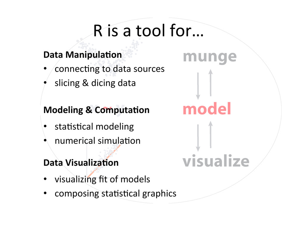
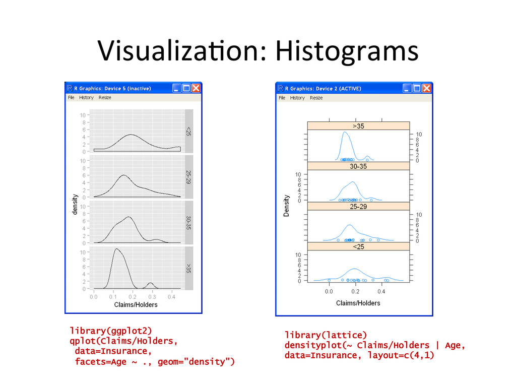
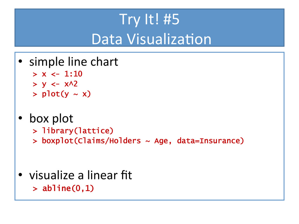
5. Modeling  &  Computa?on   •  sta$s$cal  modeling   •  numerical  simula$on   Data  Visualiza?on   R  is  a  tool  for…   Data  Manipula?on   •  connec$ng  to  data  sources   •  slicing  &  dicing  data   •  visualizing  fit  of  models   •  composing  sta$s$cal  graphics  
6. R  is  an  environment  
7. Its  interface  is  plain  
8. RStudio  to  the  rescue  
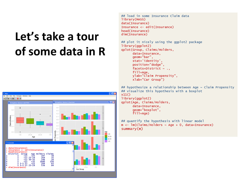
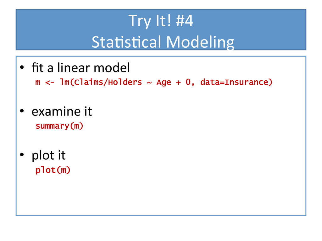
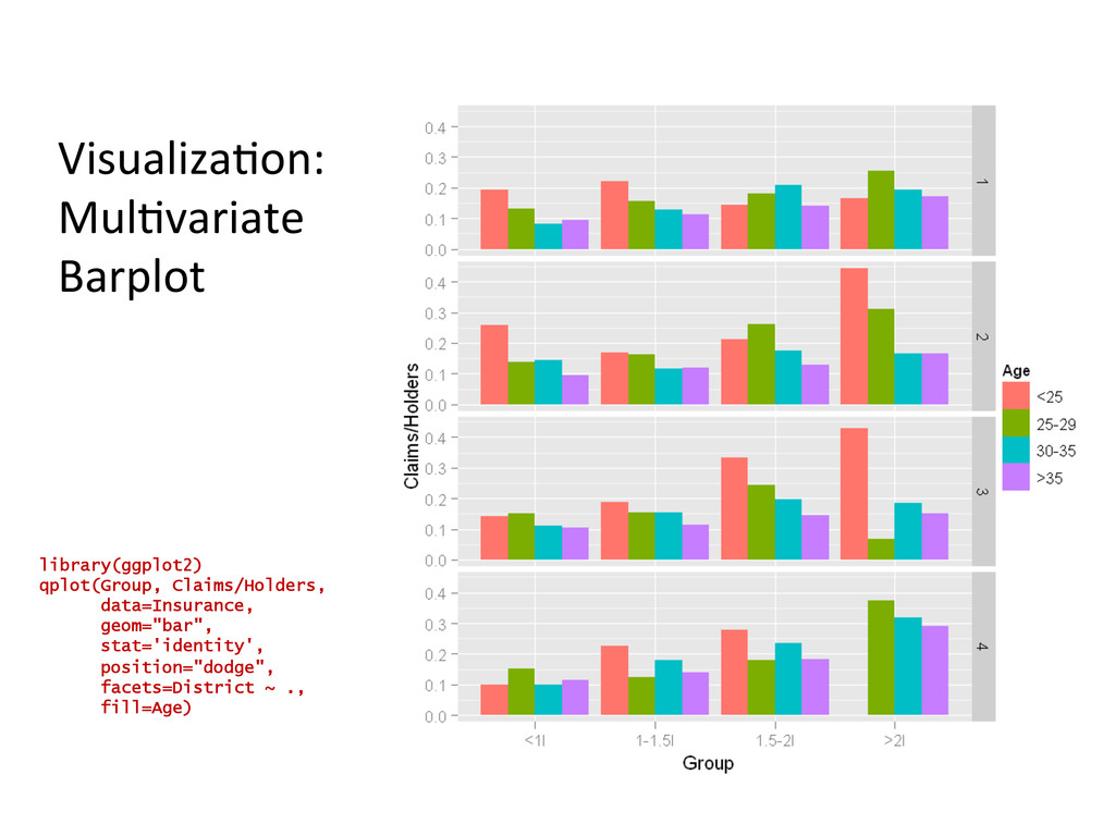
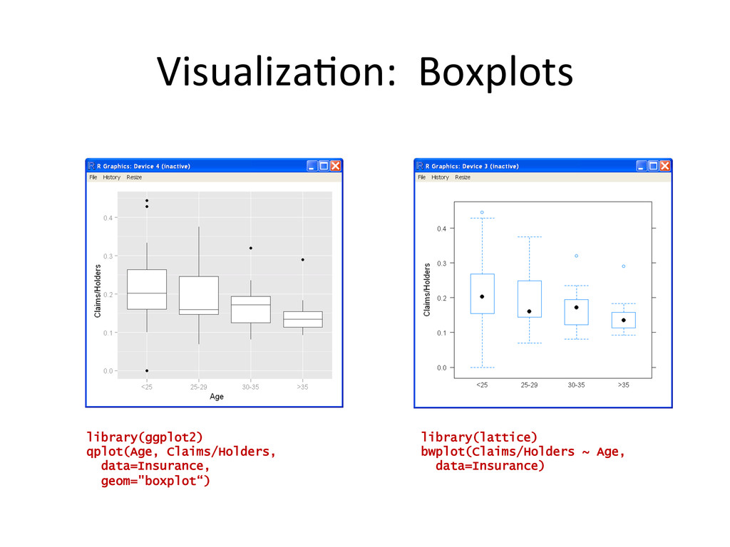
9. Let’s  take  a  tour   of  some  data  in  R   ## load in some Insurance Claim data library(MASS) data(Insurance) Insurance <- edit(Insurance) head(Insurance) dim(Insurance) ## plot it nicely using the ggplot2 package library(ggplot2) qplot(Group, Claims/Holders, data=Insurance, geom="bar", stat='identity', position="dodge", facets=District ~ ., fill=Age, ylab="Claim Propensity", xlab="Car Group") ## hypothesize a relationship between Age ~ Claim Propensity ## visualize this hypothesis with a boxplot x11() library(ggplot2) qplot(Age, Claims/Holders, data=Insurance, geom="boxplot", fill=Age) ## quantify the hypothesis with linear model m <- lm(Claims/Holders ~ Age + 0, data=Insurance) summary(m)
10. R  is  “an  overgrown  calculator”   sum(rgamma(rpois(1,lambda=2),shape=49,scale=.2)))
11. R  is  “an  overgrown  calculator”   •  simple  math   > 2+2 4 •  storing  results  in  variables   > x <- 2+2 ## ‘<-’ is R syntax for ‘=’ or assignment > x^2 16 •  vectorized  math   > weight <- c(110, 180, 240) ## three weights > height <- c(5.5, 6.1, 6.2) ## three heights > bmi <- (weight*4.88)/height^2 ## divides element-wise 17.7 23.6 30.4  
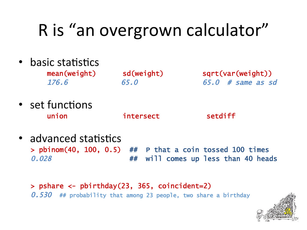
12. R  is  “an  overgrown  calculator”   •  basic  sta$s$cs   mean(weight) sd(weight) sqrt(var(weight)) 176.6 65.0 65.0 # same as sd •  set  func$ons   union intersect setdiff •  advanced  sta$s$cs   > pbinom(40, 100, 0.5) ## P that a coin tossed 100 times 0.028 ## will comes up less than 40 heads > pshare <- pbirthday(23, 365, coincident=2)   0.530 ## probability that among 23 people, two share a birthday  
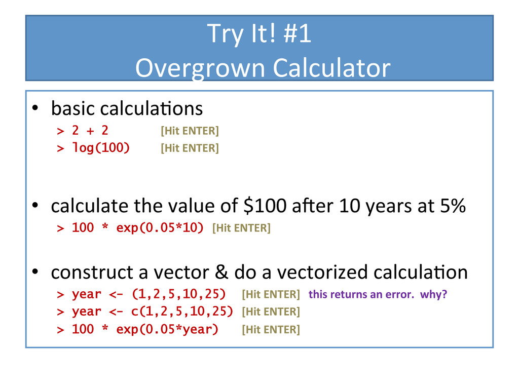
13. Try  It!  #1    Overgrown  Calculator   •  basic  calcula$ons   > 2 + 2 [Hit  ENTER] > log(100) [Hit  ENTER]   •  calculate  the  value  of  $100  aIer  10  years  at  5%   > 100 * exp(0.05*10) [Hit  ENTER] •  construct  a  vector  &  do  a  vectorized  calcula$on   > year <- (1,2,5,10,25) [Hit  ENTER]      this  returns  an  error.    why?   > year <- c(1,2,5,10,25) [Hit  ENTER] > 100 * exp(0.05*year) [Hit  ENTER]      
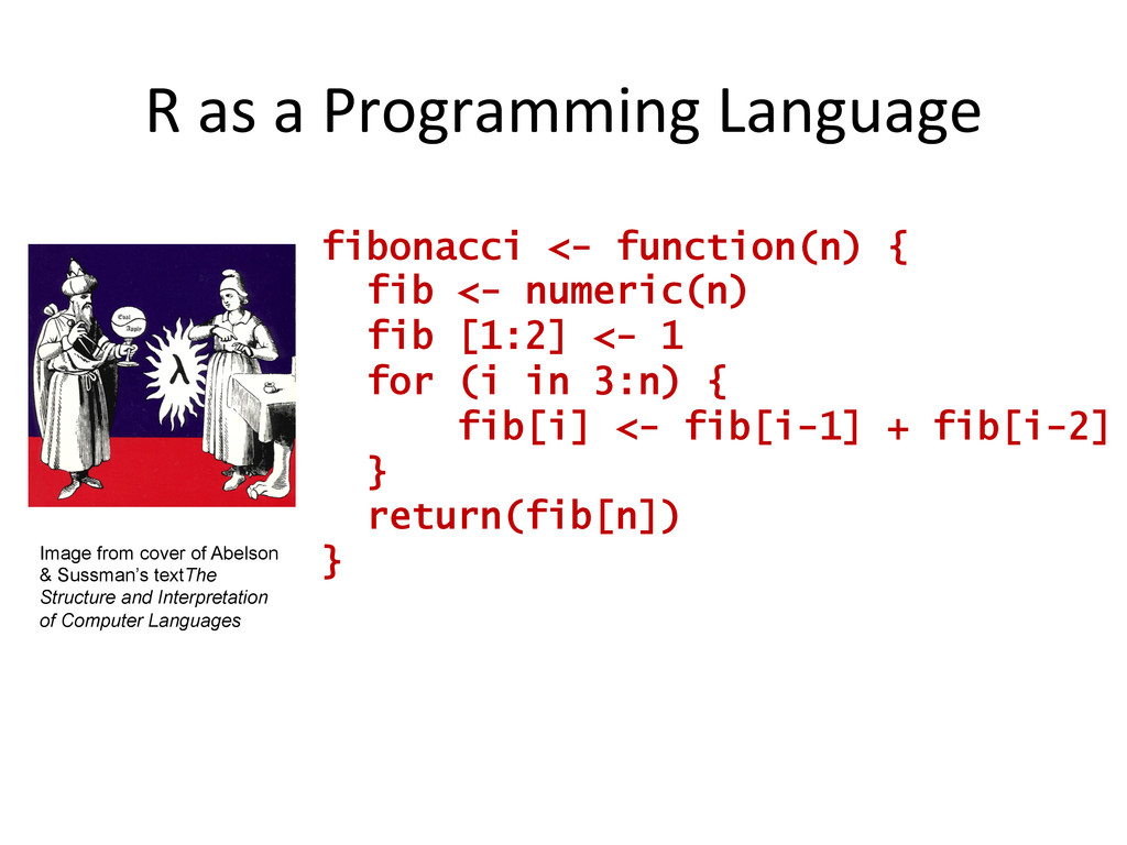
14. R  as  a  Programming  Language   fibonacci <- function(n) { fib <- numeric(n) fib [1:2] <- 1 for (i in 3:n) { fib[i] <- fib[i-1] + fib[i-2] } return(fib[n]) } Image from cover of Abelson & Sussman’s textThe Structure and Interpretation of Computer Languages
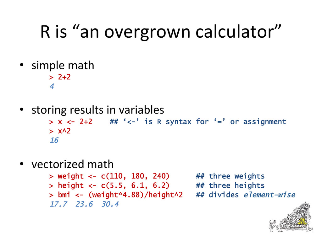
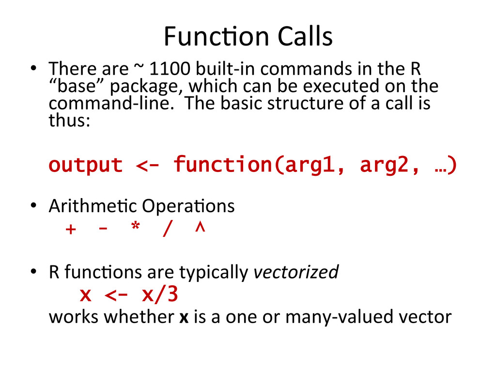
15. Func$on  Calls   •  There  are  ~  1100  built-­‐in  commands  in  the  R   “base”  package,  which  can  be  executed  on  the   command-­‐line.    The  basic  structure  of  a  call  is   thus:      output <- function(arg1, arg2, …)   •  Arithme$c  Opera$ons   + - * / ^   •  R  func$ons  are  typically  vectorized   x <- x/3  works  whether  x  is  a  one  or  many-­‐valued  vector  
16. Character   numeric   vectors   logical   x <- c(0,2:4) y <- c(“alpha”, “b”, “c3”, “4”) z <- c(1, 0, TRUE, FALSE) Data  Structures  in  R   > class(x) [1] "numeric" > x2 <- as.logical(x) > class(x2) [1] “logical”
17. matrices   lists   objects   data  frames*   lst <- list(x,y,z) M <- matrix(rep(x,3),ncol=3) df <- data.frame(x,y,z) Data  Structures  in  R   > class(df) [1] “data.frame"
18. Summary  of  Data  Structures   Linear Rectangular Homogeneous Heterogeneous data  frames*   matrices   vectors   lists   ?  
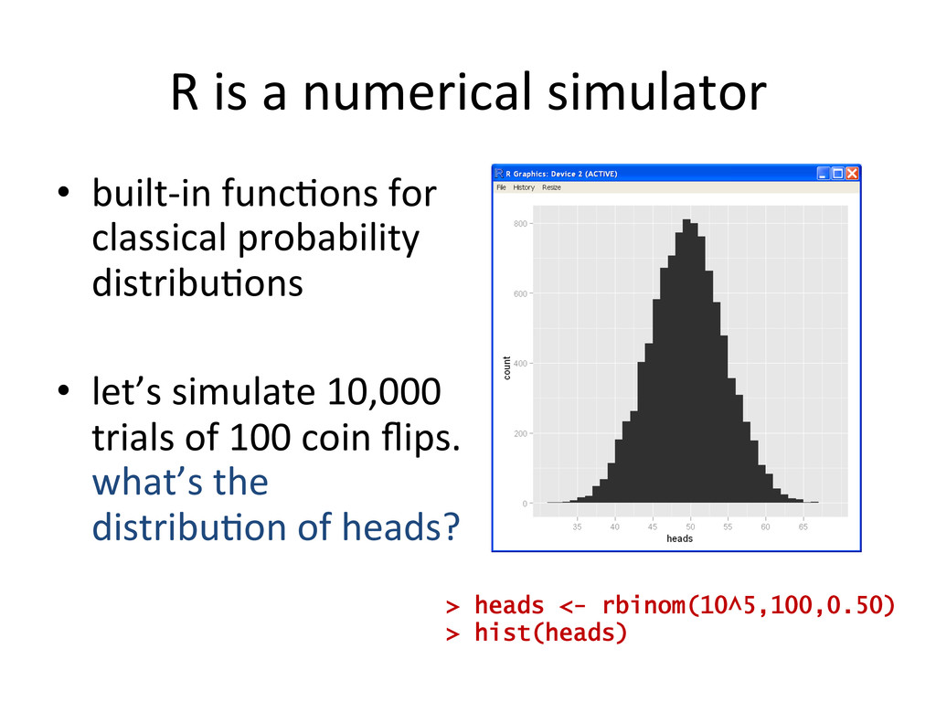
19. R  is  a  numerical  simulator     •  built-­‐in  func$ons  for   classical  probability   distribu$ons   •  let’s  simulate  10,000   trials  of  100  coin  flips.     what’s  the   distribu$on  of  heads?     > heads <- rbinom(10^5,100,0.50) > hist(heads)
20. Func$ons  for  Probability  Distribu$ons   Examples   Normal   dnorm,  pnorm,  qnorm,  rnorm   Binomial   dbinom,  pbinom,  …   Poisson   dpois,  …   ddist(  )   density  func$on  (pdf)   pdist(  )   cumula$ve  density  func$on   qdist(  )   quan$le  func$on   rdist(  )   random  deviates   >  pnorm(0)    0.05     >  qnorm(0.9)    1.28   >  rnorm(100)    vector  of  length  100    
21. Func$ons  for  Probability  Distribu$ons   distribu?on   dist  suffix  in  R   Beta   -­‐beta   Binomial   -­‐binom   Cauchy   -­‐cauchy   Chisquare   -­‐chisq   Exponen?al   -­‐exp   F   -­‐f   Gamma   -­‐gamma   Geometric   -­‐geom   Hypergeometric   -­‐hyper   Logis?c   -­‐logis   Lognormal   -­‐lnorm   Nega?ve  Binomial     -­‐nbinom   Normal   -­‐norm   Poisson   -­‐pois   Student  t     -­‐t   Uniform   -­‐unif   Tukey   -­‐tukey   Weibull   -­‐weib   Wilcoxon   -­‐wilcox   How  to  find  the  func?ons  for   lognormal  distribu?on?         1)  Use  the  double  ques$on  mark   ‘??’  to  search   > ??lognormal   2)  Then  iden$fy  the  package    >  ?Lognormal     3)  Discover  the  dist  func$ons     dlnorm, plnorm, qlnorm, rlnorm
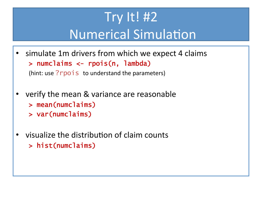
22. Try  It!  #2    Numerical  Simula$on   •  simulate  1m  drivers  from  which  we  expect  4  claims   > numclaims <- rpois(n, lambda) (hint:  use  ?rpois to  understand  the  parameters)   •  verify  the  mean  &  variance  are  reasonable > mean(numclaims) > var(numclaims) •  visualize  the  distribu$on  of  claim  counts   > hist(numclaims)    
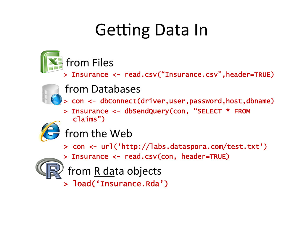
23. Gehng  Data  In    -­‐  from  Files   > Insurance <- read.csv(“Insurance.csv”,header=TRUE)      from  Databases   > con <- dbConnect(driver,user,password,host,dbname) > Insurance <- dbSendQuery(con, “SELECT * FROM claims”)      from  the  Web   > con <- url('http://labs.dataspora.com/test.txt') > Insurance <- read.csv(con, header=TRUE)        from  R  data  objects   > load(‘Insurance.Rda’)
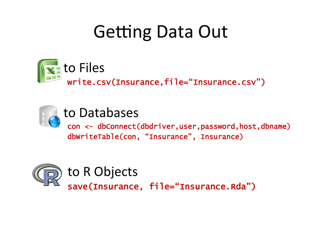
24. Gehng  Data  Out   •  to  Files   write.csv(Insurance,file=“Insurance.csv”) •  to  Databases   con <- dbConnect(dbdriver,user,password,host,dbname) dbWriteTable(con, “Insurance”, Insurance)          to  R  Objects   save(Insurance, file=“Insurance.Rda”)
25. Naviga$ng  within  the  R  environment   •  lis$ng  all  variables   > ls() •  examining  a  variable  ‘x’   > str(x) > head(x) > tail(x) > class(x) •  removing  variables   > rm(x) > rm(list=ls()) # remove everything
26. Try  It!  #3    Data  Processing     •  load  data  &  view  it   library(MASS) head(Insurance) ## the first 7 rows dim(Insurance) ## number of rows & columns •  write  it  out   write.csv(Insurance,file=“Insurance.csv”, row.names=FALSE) getwd() ## where am I? •  view  it  in  Excel,  make  a  change,  save  it   remove the first district   •  load  it  back  in  to  R  &  plot  it   Insurance <- read.csv(file=“Insurance.csv”) plot(Claims/Holders ~ Age, data=Insurance)
27. A  Swiss-­‐Army  Knife  for  Data  
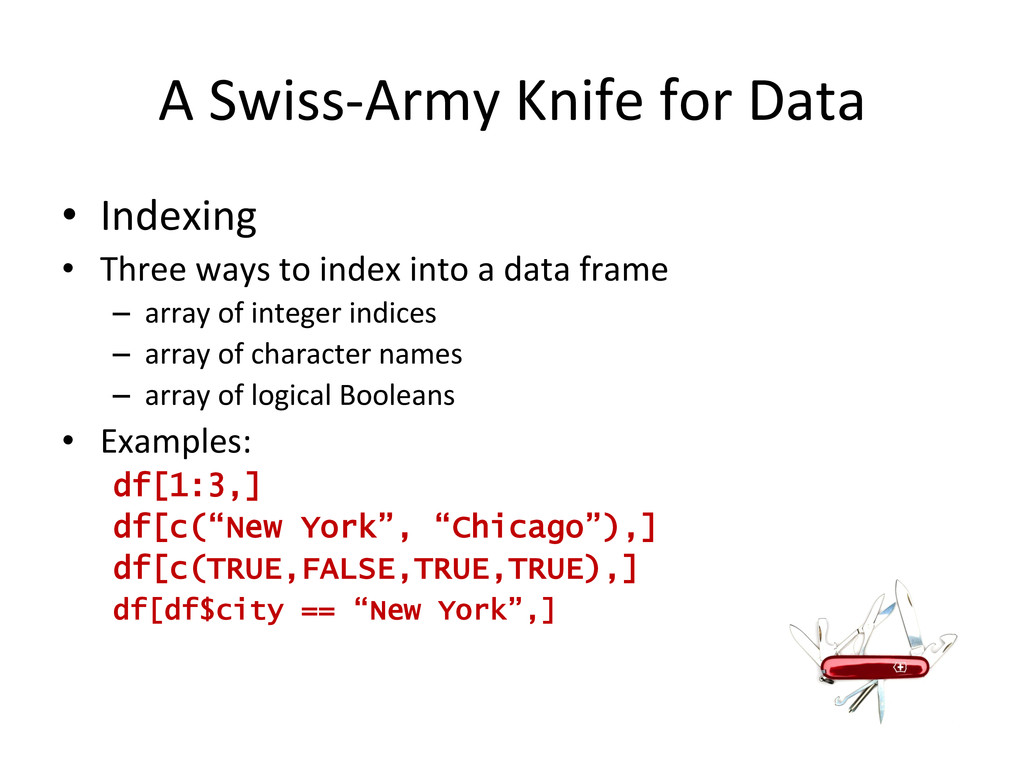
28. A  Swiss-­‐Army  Knife  for  Data   •  Indexing   •  Three  ways  to  index  into  a  data  frame   –  array  of  integer  indices   –  array  of  character  names   –  array  of  logical  Booleans   •  Examples:   df[1:3,] df[c(“New York”, “Chicago”),] df[c(TRUE,FALSE,TRUE,TRUE),] df[df$city == “New York”,]
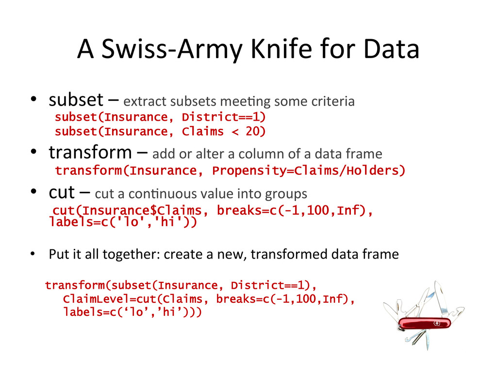
29. A  Swiss-­‐Army  Knife  for  Data   •  subset  –  extract  subsets  mee$ng  some  criteria   subset(Insurance, District==1) subset(Insurance, Claims < 20) •  transform  –  add  or  alter  a  column  of  a  data  frame   transform(Insurance, Propensity=Claims/Holders) •  cut  –  cut  a  con$nuous  value  into  groups cut(Insurance$Claims, breaks=c(-1,100,Inf), labels=c('lo','hi')) •  Put  it  all  together:  create  a  new,  transformed  data  frame   transform(subset(Insurance, District==1), ClaimLevel=cut(Claims, breaks=c(-1,100,Inf), labels=c(‘lo’,’hi’)))  
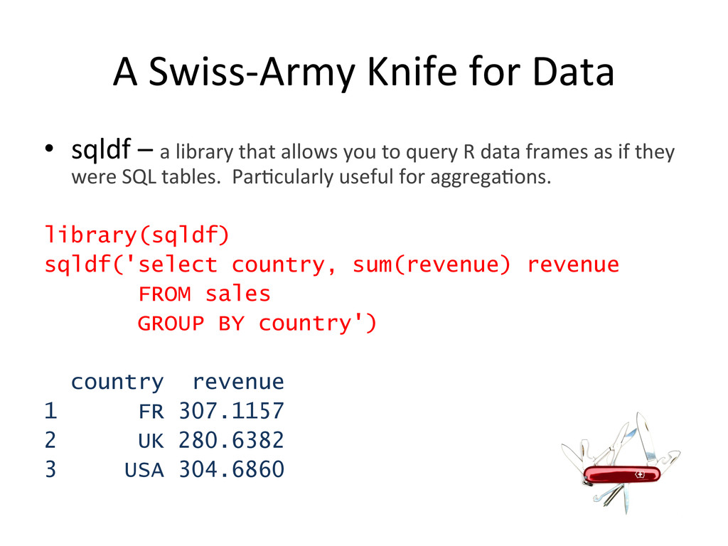
30. A  Swiss-­‐Army  Knife  for  Data   •  sqldf  –  a  library  that  allows  you  to  query  R  data  frames  as  if  they   were  SQL  tables.    Par$cularly  useful  for  aggrega$ons.   library(sqldf) sqldf('select country, sum(revenue) revenue FROM sales GROUP BY country') country revenue 1 FR 307.1157 2 UK 280.6382 3 USA 304.6860
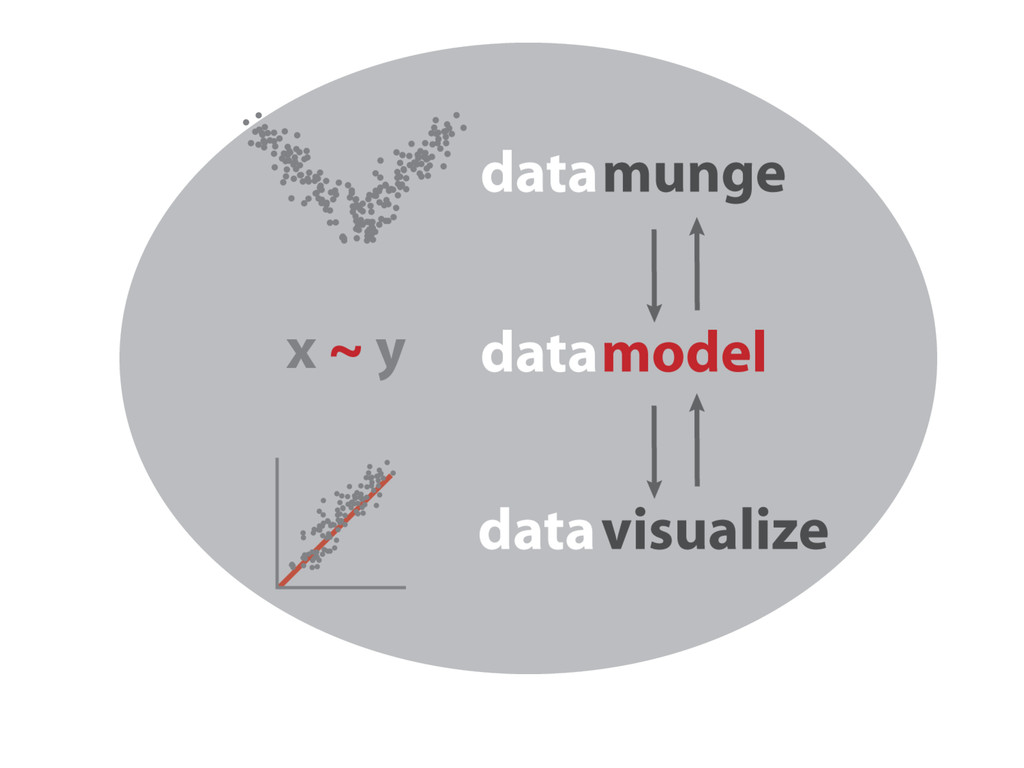
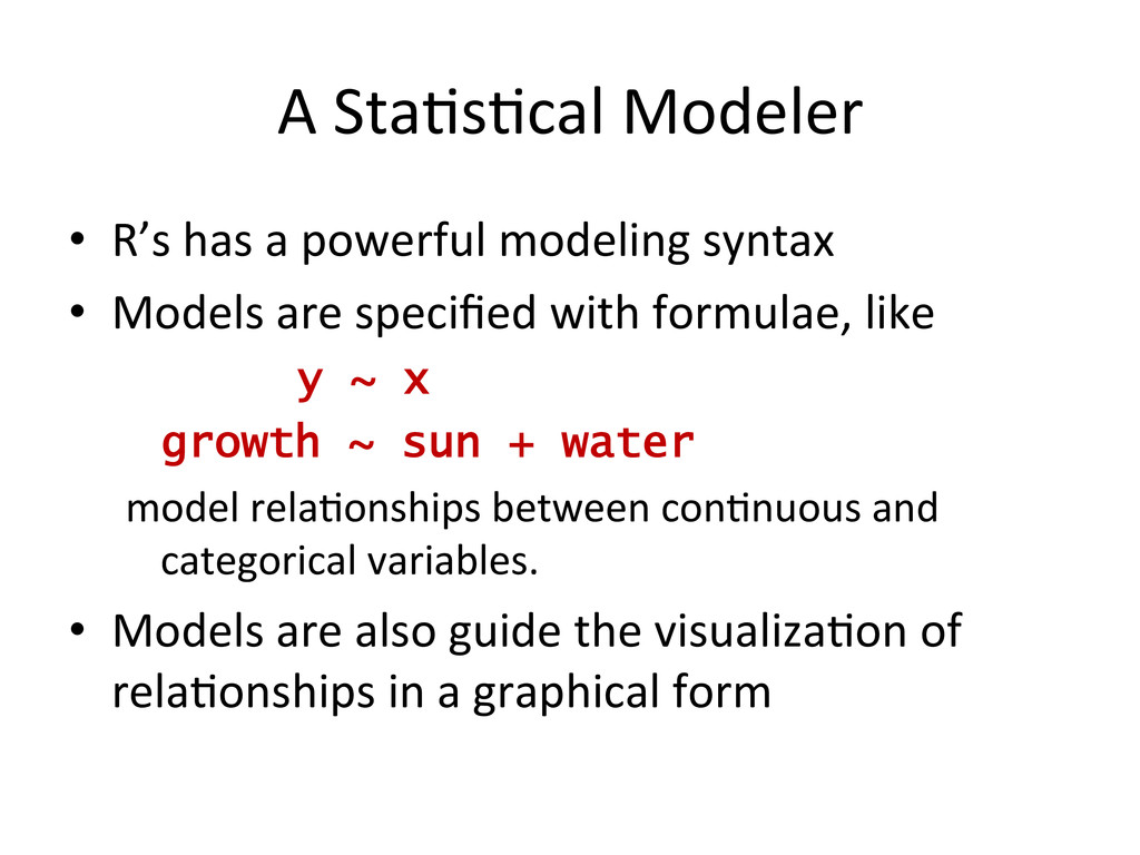
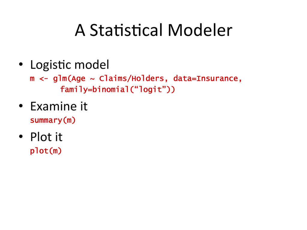
31. A  Sta$s$cal  Modeler   •  R’s  has  a  powerful  modeling  syntax   •  Models  are  specified  with  formulae,  like     y ~ x growth ~ sun + water model  rela$onships  between  con$nuous  and   categorical  variables.   •  Models  are  also  guide  the  visualiza$on  of   rela$onships  in  a  graphical  form  
32. A  Sta$s$cal  Modeler   •  Linear  model   m <- lm(Claims/Holders ~ Age, data=Insurance) •  Examine  it   summary(m) •  Plot  it   plot(m)
33. A  Sta$s$cal  Modeler   •  Logis$c  model   m <- glm(Age ~ Claims/Holders, data=Insurance, family=binomial(“logit”)) •  Examine  it   summary(m) •  Plot  it   plot(m)
34. Try  It!  #4    Sta$s$cal  Modeling   •  fit  a  linear  model   m <- lm(Claims/Holders ~ Age + 0, data=Insurance) •  examine  it     summary(m)   •  plot  it   plot(m)
35. Visualiza$on:       Mul$variate   Barplot   library(ggplot2) qplot(Group, Claims/Holders, data=Insurance, geom="bar", stat='identity', position="dodge", facets=District ~ ., fill=Age)
36. Visualiza$on:    Boxplots   library(ggplot2) qplot(Age, Claims/Holders, data=Insurance, geom="boxplot“)   library(lattice) bwplot(Claims/Holders ~ Age, data=Insurance)
37. Visualiza$on:  Histograms   library(lattice) densityplot(~ Claims/Holders | Age, data=Insurance, layout=c(4,1) library(ggplot2) qplot(Claims/Holders, data=Insurance, facets=Age ~ ., geom="density")
38. Try  It!  #5    Data  Visualiza$on   •  simple  line  chart   > x <- 1:10 > y <- x^2 > plot(y ~ x) •  box  plot   > library(lattice) > boxplot(Claims/Holders ~ Age, data=Insurance)   •  visualize  a  linear  fit   > abline(0,1)
39. Gehng  Help  with  R   Help  within  R  itself  for  a  func?on   > help(func) > ?func For  a  topic   > help.search(topic) > ??topic   •  search.r-­‐project.org   •  Google  Code  Search    www.google.com/codesearch   •  Stack  Overflow    hsp://stackoverflow.com/tags/R     •  R-­‐help  list  hsp://www.r-­‐project.org/pos$ng-­‐guide.html    
40. Six  Indispensable  Books  on  R   Visualiza?on:      la-ce  &  ggplot2   Learning  R   Sta?s?cal  Modeling   Data  Manipula?on  
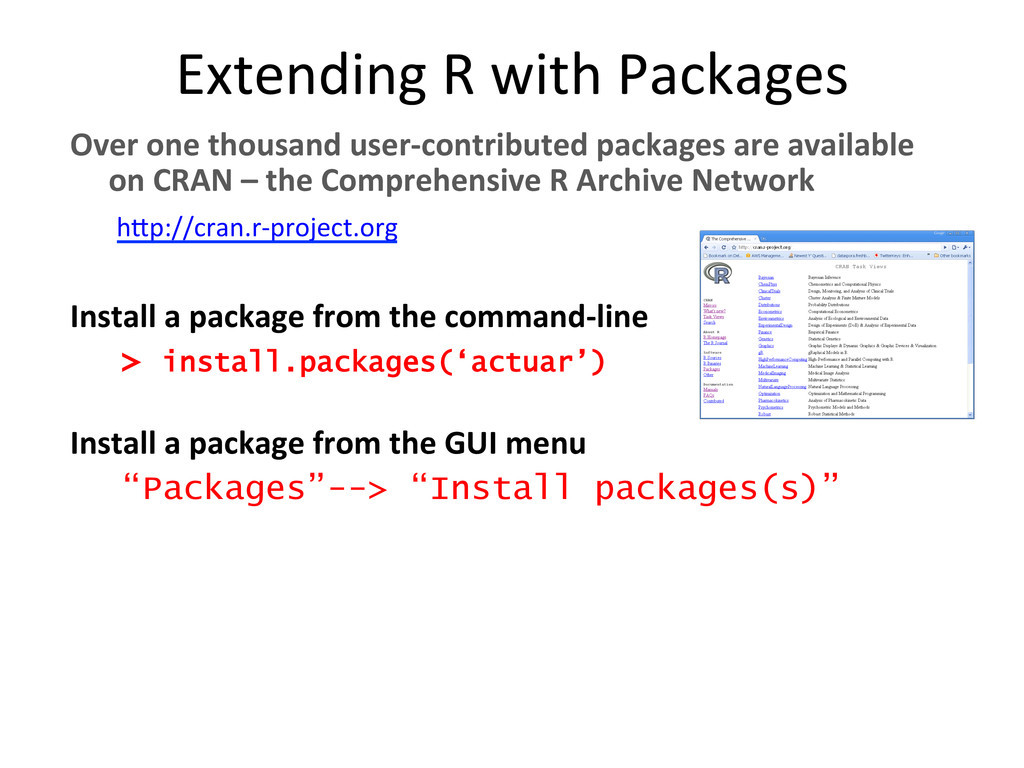
41. Extending  R  with  Packages   Over  one  thousand  user-­‐contributed  packages  are  available   on  CRAN  –  the  Comprehensive  R  Archive  Network              hsp://cran.r-­‐project.org       Install  a  package  from  the  command-­‐line   > install.packages(‘actuar’) Install  a  package  from  the  GUI  menu   “Packages”--> “Install packages(s)”
42. Visualiza?on  with   lagce  
43. lahce  =  trellis   (source:  hsp://lmdvr.r-­‐forge.r-­‐project.org  )  
44. densityplot(~ speed | type, data=pitch)   list  of     lahce   func$ons  
45. Visualiza?on  with     ggplot2  
46. ggplot2  =   grammar  of     graphics  
47. ggplot2  =   grammar  of   graphics  
48. Visualizing  50,000  Diamonds  with  ggplot2  
49. qplot(carat, price, data = diamonds)
50. qplot(log(carat), log(price), data = diamonds)
51. qplot(log(carat), log(price), data = diamonds, alpha = I(1/20))
52. qplot(log(carat), log(price), data = diamonds, alpha = I(1/20), colour=color)
53. qplot(log(carat), log(price), data = diamonds, alpha=I(1/20)) + facet_grid(. ~ color)
54. qplot(color, price/carat, data = diamonds, alpha = I(1/20), geom=“jitter”) qplot(color, price/carat, data = diamonds, geom=“boxplot”)
56. (live  demo)  
57. visualizing  six  dimensions   of  MLB  pitches  with  ggplot2  
58. Demo  with  MLB  Gameday  Data   Code, data, and instructions at: http://metamx-mdriscol-adhoc.s3.amazonaws.com/gameday/README.R