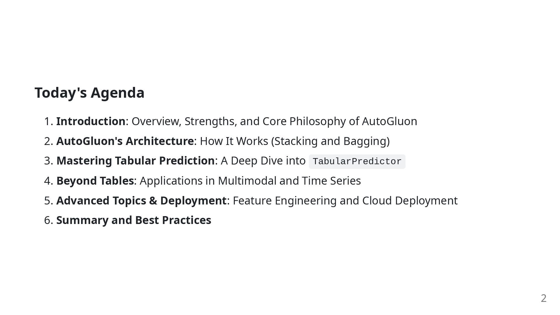
AutoGluon 2. AutoGluon's Architecture: How It Works (Stacking and Bagging) 3. Mastering Tabular Prediction: A Deep Dive into TabularPredictor 4. Beyond Tables: Applications in Multimodal and Time Series 5. Advanced Topics & Deployment: Feature Engineering and Cloud Deployment 6. Summary and Best Practices 2
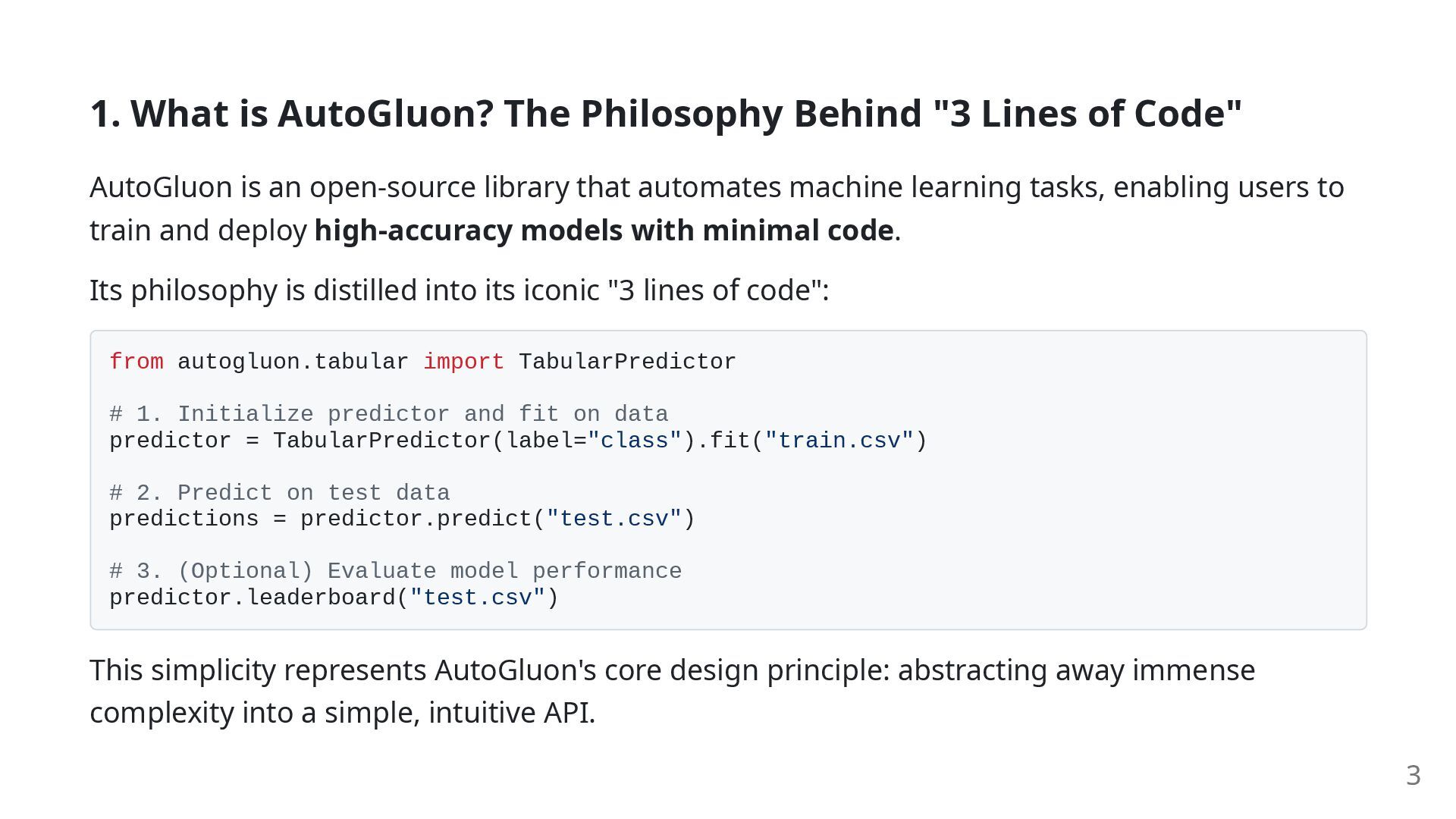
Code" AutoGluon is an open-source library that automates machine learning tasks, enabling users to train and deploy high-accuracy models with minimal code. Its philosophy is distilled into its iconic "3 lines of code": from autogluon.tabular import TabularPredictor # 1. Initialize predictor and fit on data predictor = TabularPredictor(label="class").fit("train.csv") # 2. Predict on test data predictions = predictor.predict("test.csv") # 3. (Optional) Evaluate model performance predictor.leaderboard("test.csv") This simplicity represents AutoGluon's core design principle: abstracting away immense complexity into a simple, intuitive API. 3
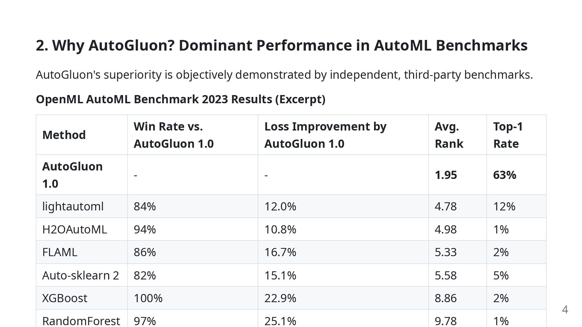
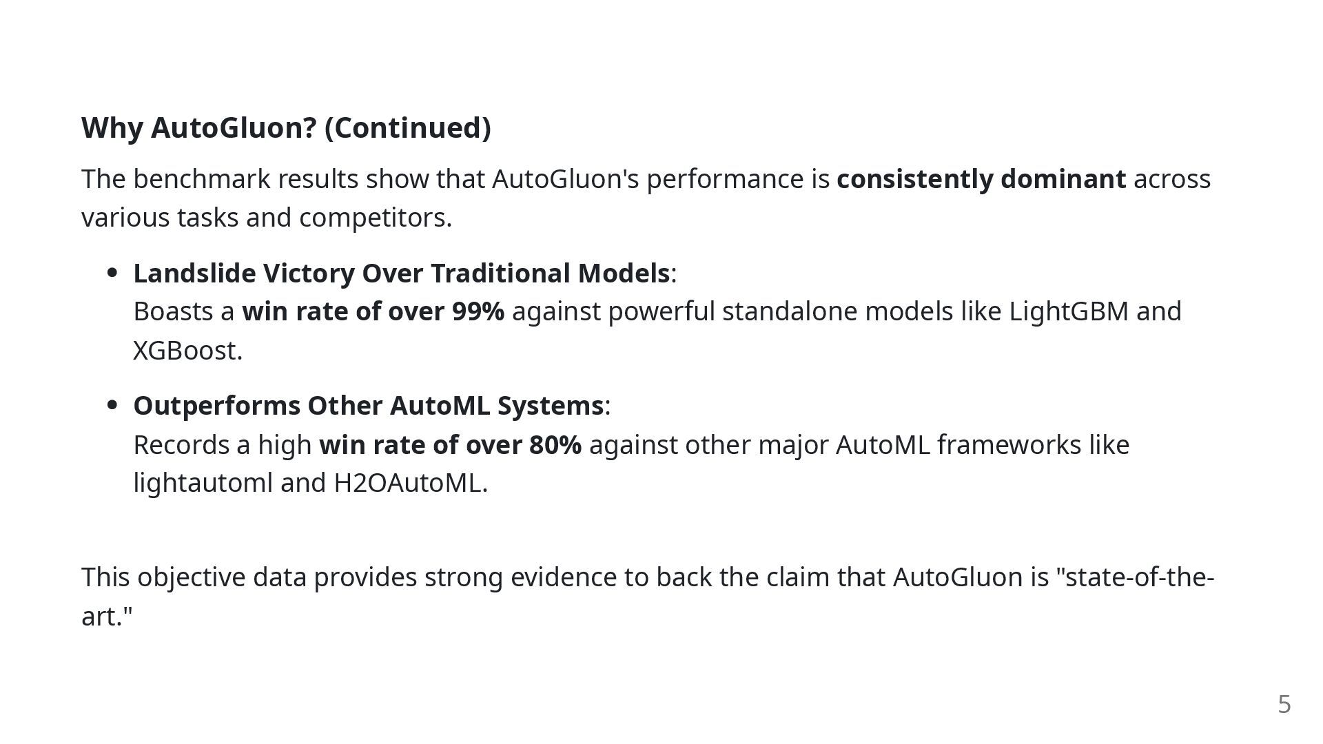
is consistently dominant across various tasks and competitors. Landslide Victory Over Traditional Models: Boasts a win rate of over 99% against powerful standalone models like LightGBM and XGBoost. Outperforms Other AutoML Systems: Records a high win rate of over 80% against other major AutoML frameworks like lightautoml and H2OAutoML. This objective data provides strong evidence to back the claim that AutoGluon is "state-of-the- art." 5
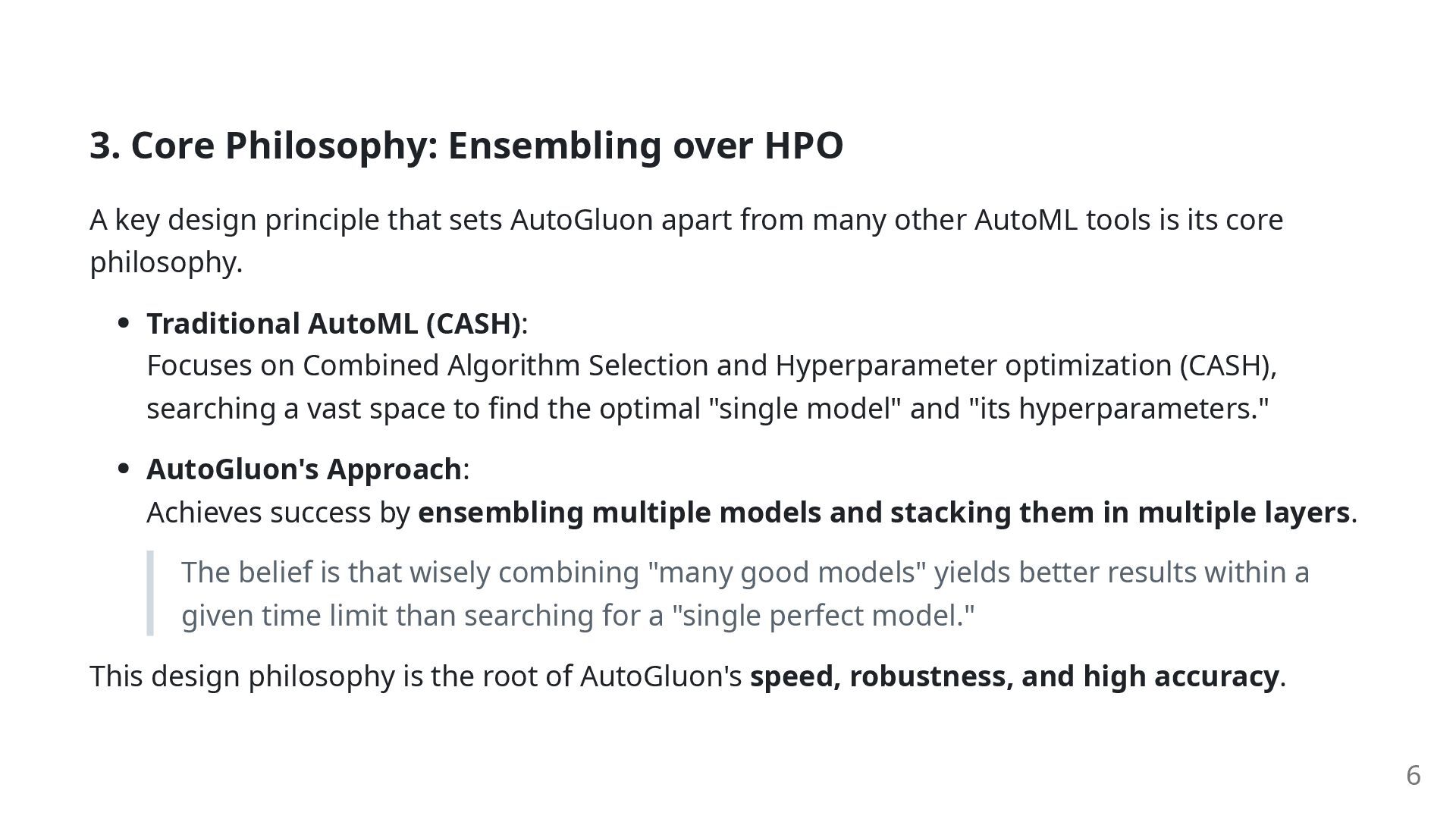
that sets AutoGluon apart from many other AutoML tools is its core philosophy. Traditional AutoML (CASH): Focuses on Combined Algorithm Selection and Hyperparameter optimization (CASH), searching a vast space to find the optimal "single model" and "its hyperparameters." AutoGluon's Approach: Achieves success by ensembling multiple models and stacking them in multiple layers. The belief is that wisely combining "many good models" yields better results within a given time limit than searching for a "single perfect model." This design philosophy is the root of AutoGluon's speed, robustness, and high accuracy. 6
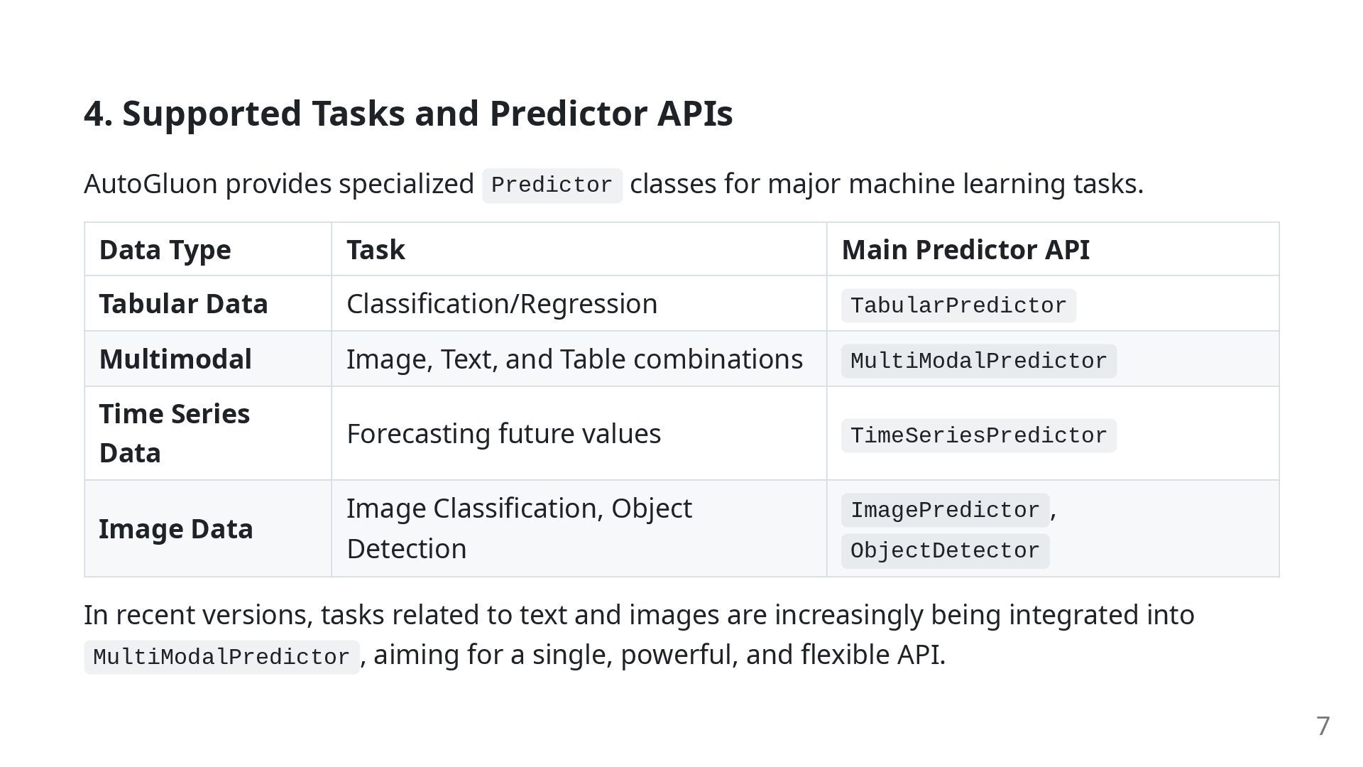
classes for major machine learning tasks. Data Type Task Main Predictor API Tabular Data Classification/Regression TabularPredictor Multimodal Image, Text, and Table combinations MultiModalPredictor Time Series Data Forecasting future values TimeSeriesPredictor Image Data Image Classification, Object Detection ImagePredictor , ObjectDetector In recent versions, tasks related to text and images are increasingly being integrated into MultiModalPredictor , aiming for a single, powerful, and flexible API. 7
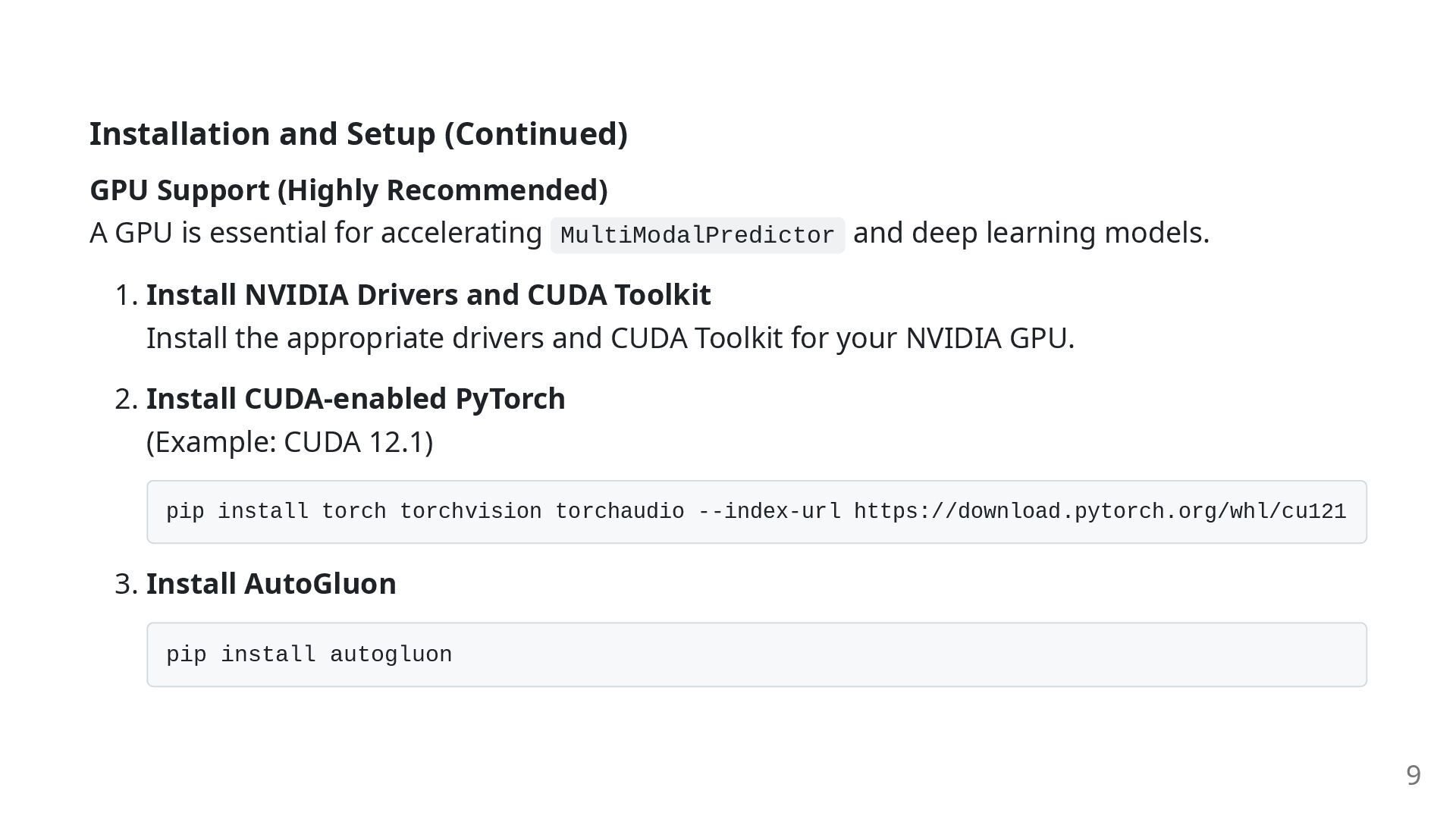
is essential for accelerating MultiModalPredictor and deep learning models. 1. Install NVIDIA Drivers and CUDA Toolkit Install the appropriate drivers and CUDA Toolkit for your NVIDIA GPU. 2. Install CUDA-enabled PyTorch (Example: CUDA 12.1) pip install torch torchvision torchaudio --index-url https://download.pytorch.org/whl/cu121 3. Install AutoGluon pip install autogluon 9
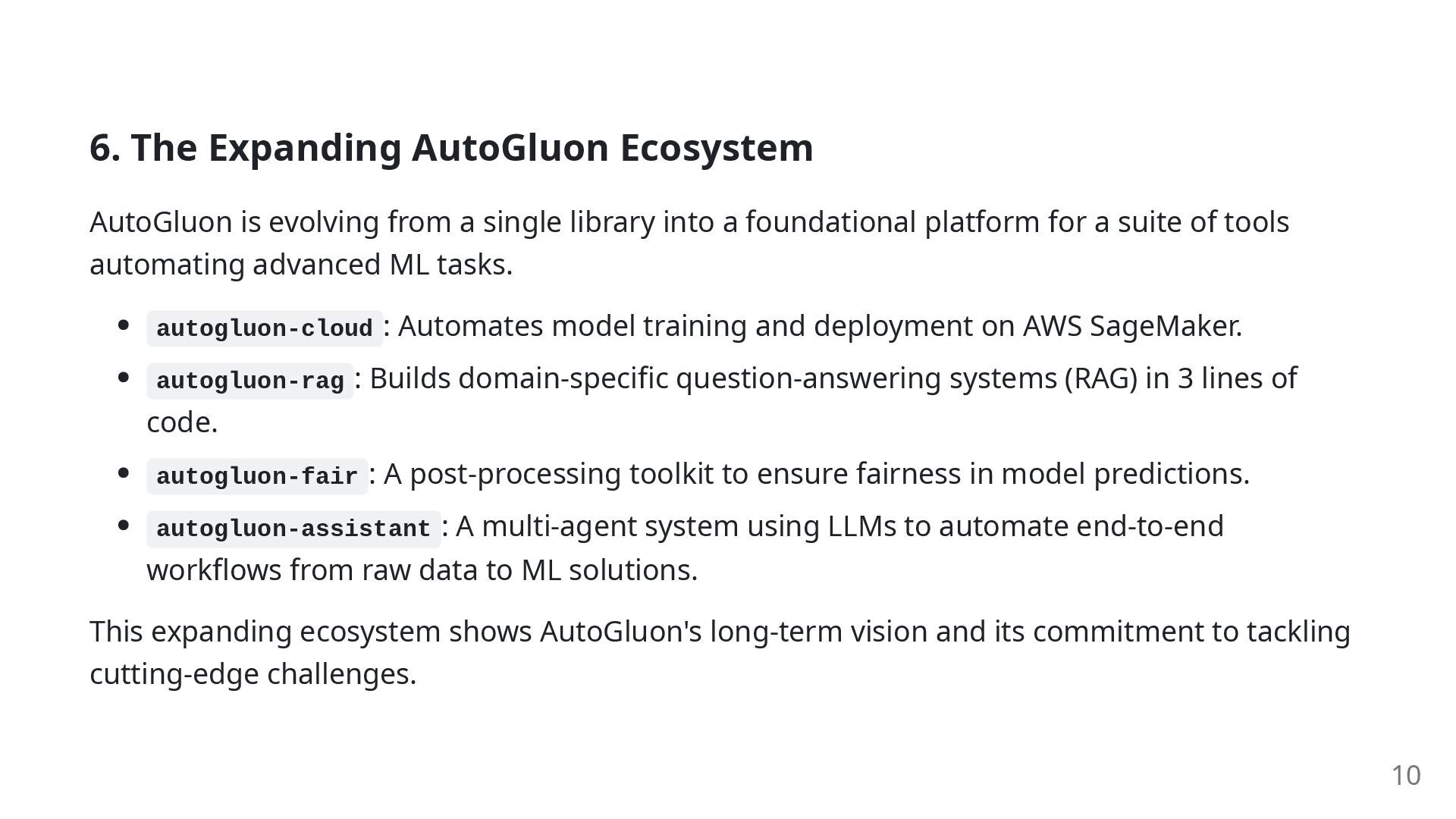
single library into a foundational platform for a suite of tools automating advanced ML tasks. autogluon-cloud : Automates model training and deployment on AWS SageMaker. autogluon-rag : Builds domain-specific question-answering systems (RAG) in 3 lines of code. autogluon-fair : A post-processing toolkit to ensure fairness in model predictions. autogluon-assistant : A multi-agent system using LLMs to automate end-to-end workflows from raw data to ML solutions. This expanding ecosystem shows AutoGluon's long-term vision and its commitment to tackling cutting-edge challenges. 10
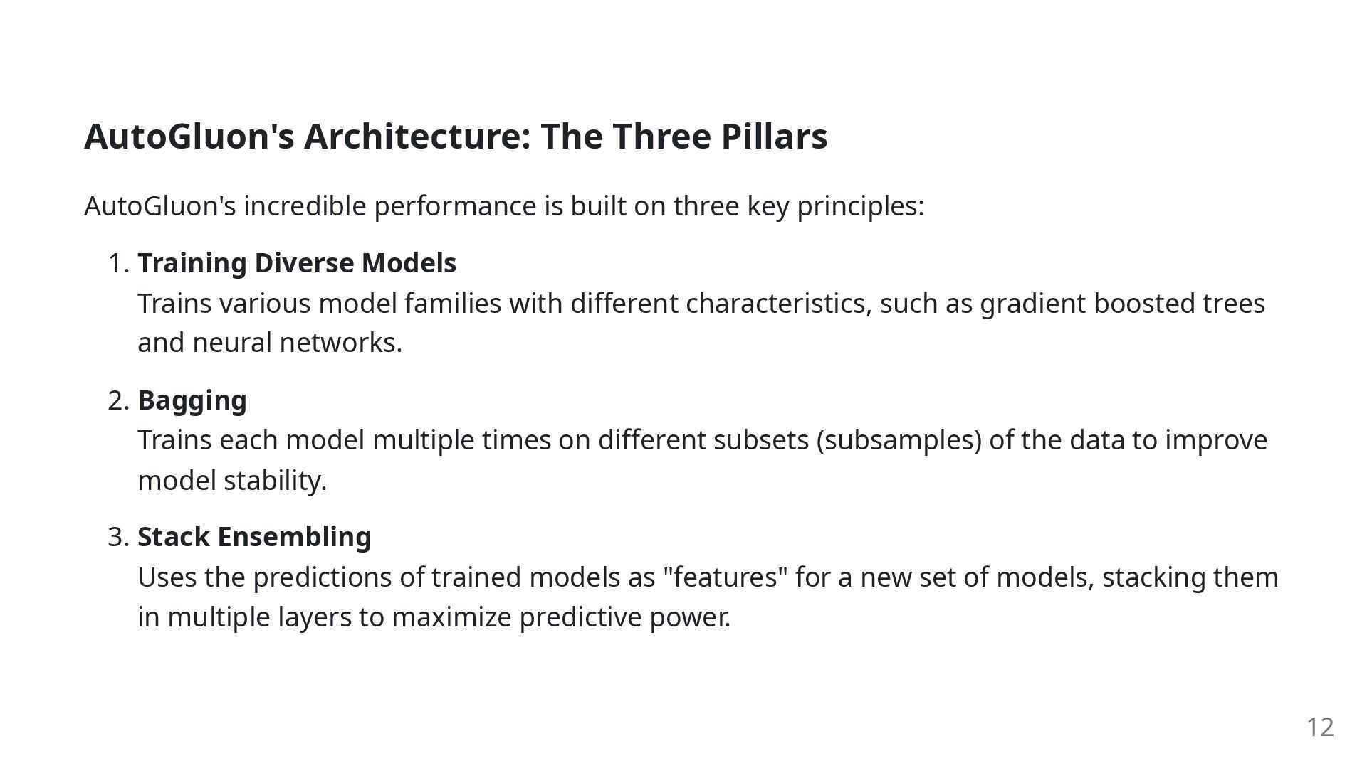
on three key principles: 1. Training Diverse Models Trains various model families with different characteristics, such as gradient boosted trees and neural networks. 2. Bagging Trains each model multiple times on different subsets (subsamples) of the data to improve model stability. 3. Stack Ensembling Uses the predictions of trained models as "features" for a new set of models, stacking them in multiple layers to maximize predictive power. 12
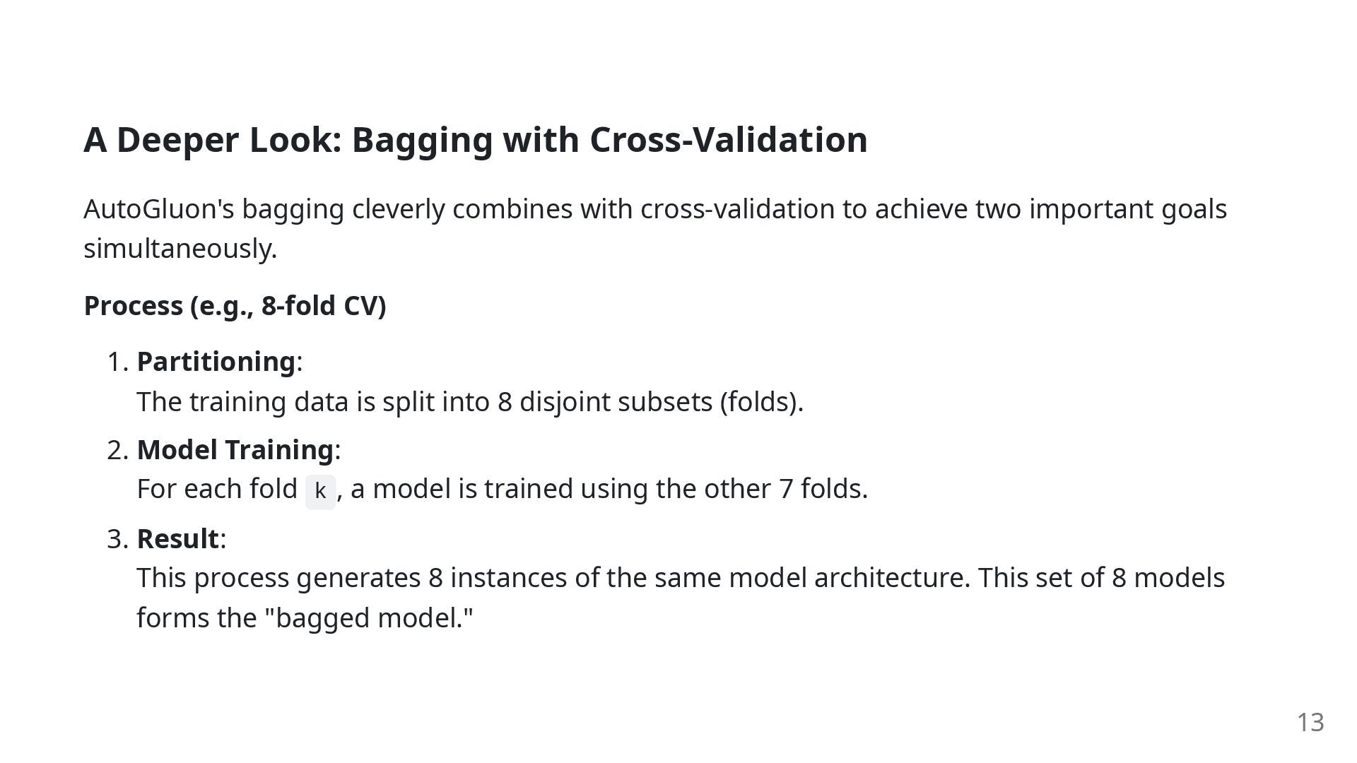
with cross-validation to achieve two important goals simultaneously. Process (e.g., 8-fold CV) 1. Partitioning: The training data is split into 8 disjoint subsets (folds). 2. Model Training: For each fold k , a model is trained using the other 7 folds. 3. Result: This process generates 8 instances of the same model architecture. This set of 8 models forms the "bagged model." 13
in its by-product. Variance Reduction (The primary purpose of bagging): By averaging the predictions of multiple models, the final prediction is more stable and less prone to overfitting than a single model's prediction. Generation of Out-of-Fold (OOF) Predictions: For each data point, we get a "clean" prediction made by a model that was not trained on that data point. These OOF predictions are the key to making the next step, stack ensembling, work robustly. 14
(OOF) predictions? For each data point in the training set, it is the prediction made by a model that did not see that data point during its training. Why are they crucial? They are essential to prevent data leakage. If a stacker model were to train on the in-sample predictions of a base model (i.e., predictions on data the base model has already seen), the stacker would learn to over-trust these predictions, leading to severe overfitting and poor performance on unseen data. OOF predictions simulate how a model behaves on unseen data, creating a reliable and valid feature set for the next layer of models. 15
a technique that uses the predictions of models as new features, stacking them in a hierarchical structure. Layer 1 (Base Layer): Multiple bagged models (LightGBM, CatBoost, NN, etc.) are trained using only the original features. These models generate OOF predictions. Layer 2 (Stacker Layer): 16
in each layer receive "original features + OOF predictions from all lower layers" as input. Why is this powerful? The higher-layer models learn how to combine the predictions of the lower-layer models. At the same time, they can directly capture patterns in the original data that all lower- layer models might have missed. This prevents information loss and maximizes predictive power. 17
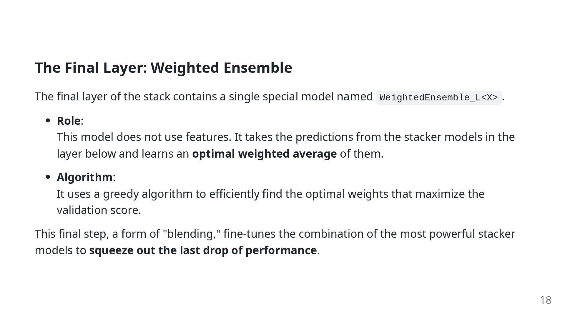
stack contains a single special model named WeightedEnsemble_L<X> . Role: This model does not use features. It takes the predictions from the stacker models in the layer below and learns an optimal weighted average of them. Algorithm: It uses a greedy algorithm to efficiently find the optimal weights that maximize the validation score. This final step, a form of "blending," fine-tunes the combination of the most powerful stacker models to squeeze out the last drop of performance. 18
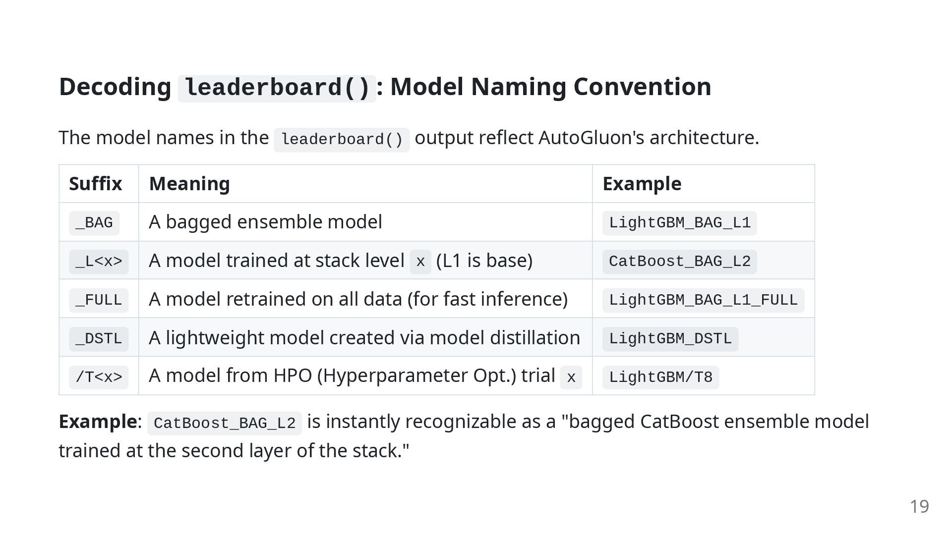
the leaderboard() output reflect AutoGluon's architecture. Suffix Meaning Example _BAG A bagged ensemble model LightGBM_BAG_L1 _L<x> A model trained at stack level x (L1 is base) CatBoost_BAG_L2 _FULL A model retrained on all data (for fast inference) LightGBM_BAG_L1_FULL _DSTL A lightweight model created via model distillation LightGBM_DSTL /T<x> A model from HPO (Hyperparameter Opt.) trial x LightGBM/T8 Example: CatBoost_BAG_L2 is instantly recognizable as a "bagged CatBoost ensemble model trained at the second layer of the stack." 19
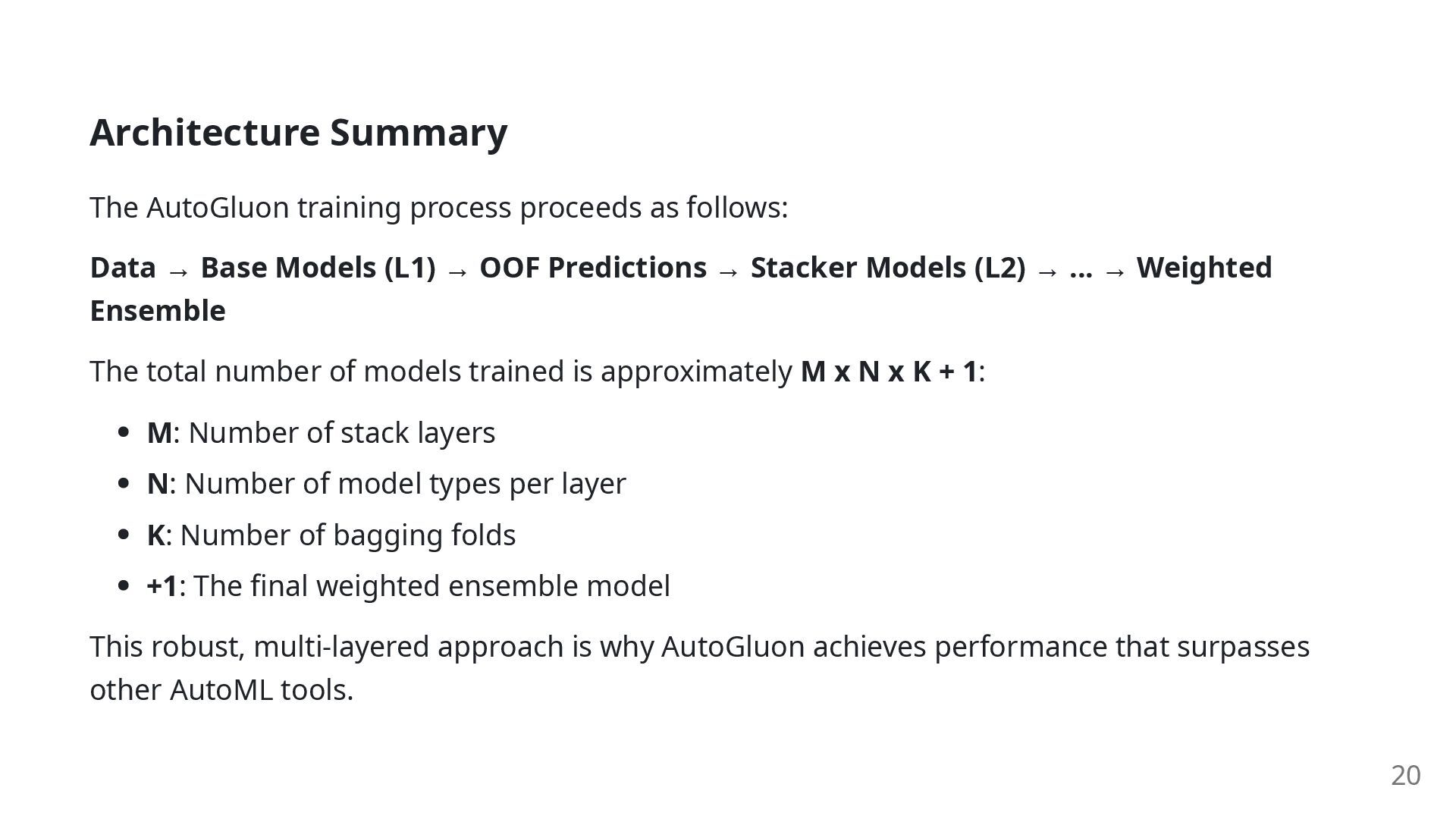
→ Base Models (L1) → OOF Predictions → Stacker Models (L2) → ... → Weighted Ensemble The total number of models trained is approximately M x N x K + 1: M: Number of stack layers N: Number of model types per layer K: Number of bagging folds +1: The final weighted ensemble model This robust, multi-layered approach is why AutoGluon achieves performance that surpasses other AutoML tools. 20
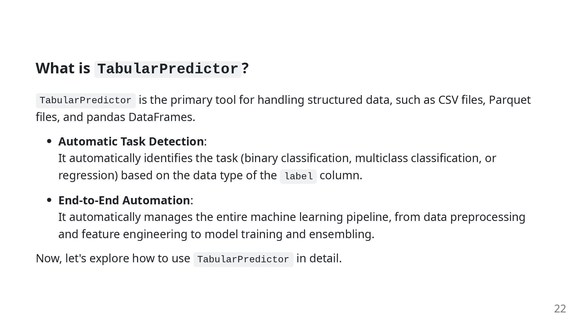
handling structured data, such as CSV files, Parquet files, and pandas DataFrames. Automatic Task Detection: It automatically identifies the task (binary classification, multiclass classification, or regression) based on the data type of the label column. End-to-End Automation: It automatically manages the entire machine learning pipeline, from data preprocessing and feature engineering to model training and ensembling. Now, let's explore how to use TabularPredictor in detail. 22
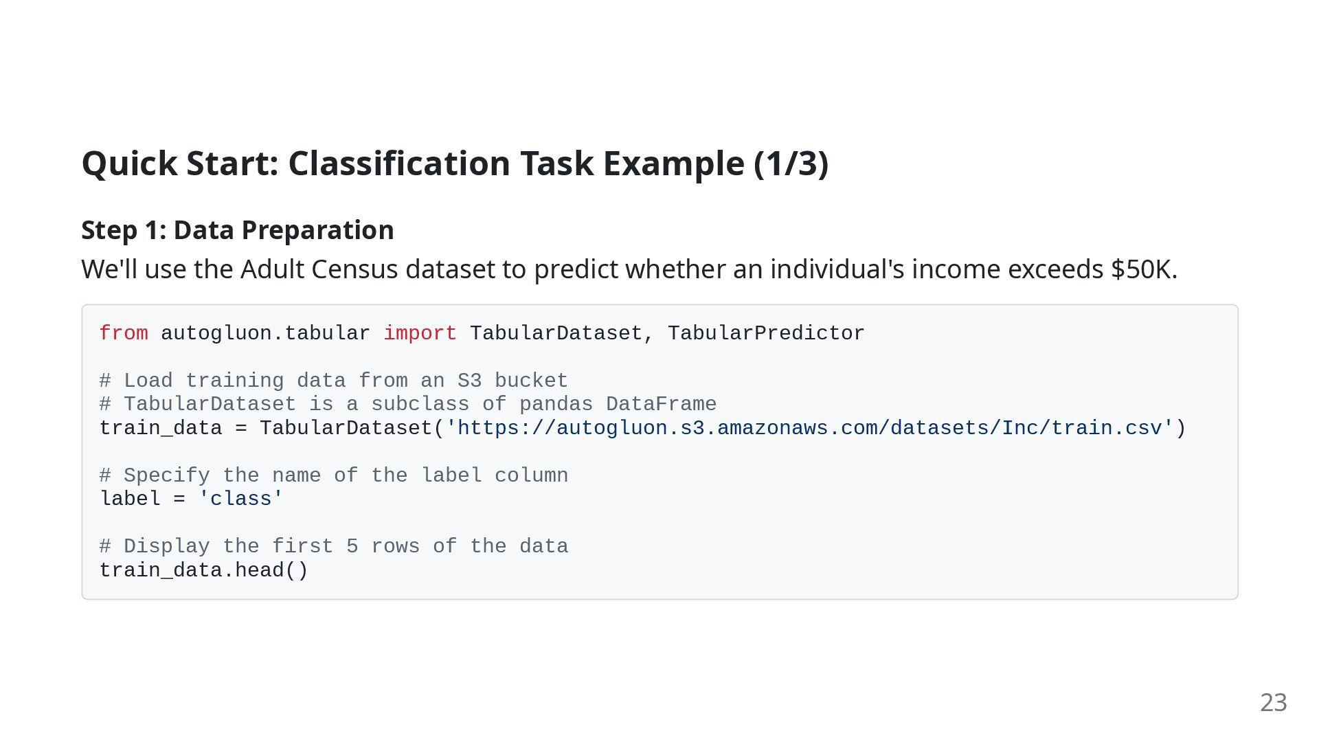
We'll use the Adult Census dataset to predict whether an individual's income exceeds $50K. from autogluon.tabular import TabularDataset, TabularPredictor # Load training data from an S3 bucket # TabularDataset is a subclass of pandas DataFrame train_data = TabularDataset('https://autogluon.s3.amazonaws.com/datasets/Inc/train.csv') # Specify the name of the label column label = 'class' # Display the first 5 rows of the data train_data.head() 23
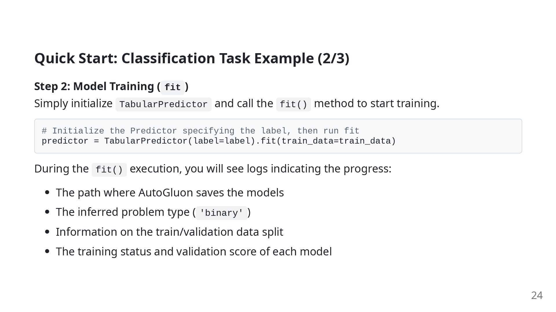
( fit ) Simply initialize TabularPredictor and call the fit() method to start training. # Initialize the Predictor specifying the label, then run fit predictor = TabularPredictor(label=label).fit(train_data=train_data) During the fit() execution, you will see logs indicating the progress: The path where AutoGluon saves the models The inferred problem type ( 'binary' ) Information on the train/validation data split The training status and validation score of each model 24
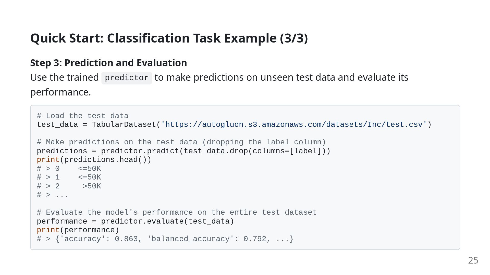
Evaluation Use the trained predictor to make predictions on unseen test data and evaluate its performance. # Load the test data test_data = TabularDataset('https://autogluon.s3.amazonaws.com/datasets/Inc/test.csv') # Make predictions on the test data (dropping the label column) predictions = predictor.predict(test_data.drop(columns=[label])) print(predictions.head()) # > 0 <=50K # > 1 <=50K # > 2 >50K # > ... # Evaluate the model's performance on the entire test dataset performance = predictor.evaluate(test_data) print(performance) # > {'accuracy': 0.863, 'balanced_accuracy': 0.792, ...} 25
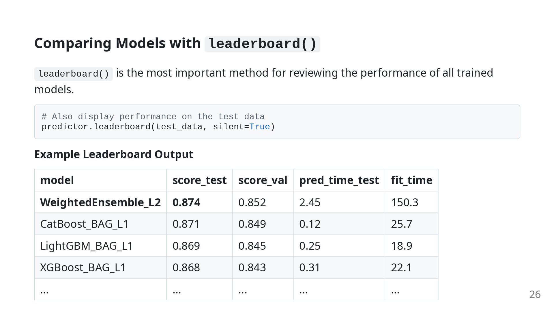
for reviewing the performance of all trained models. # Also display performance on the test data predictor.leaderboard(test_data, silent=True) Example Leaderboard Output model score_test score_val pred_time_test fit_time WeightedEnsemble_L2 0.874 0.852 2.45 150.3 CatBoost_BAG_L1 0.871 0.849 0.12 25.7 LightGBM_BAG_L1 0.869 0.845 0.25 18.9 XGBoost_BAG_L1 0.868 0.843 0.31 22.1 ... ... ... ... ... 26
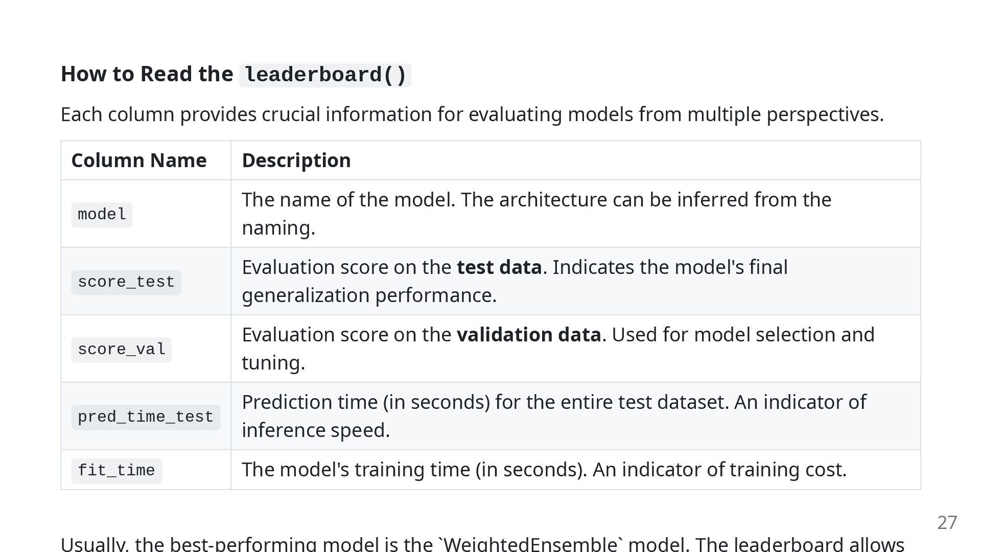
for evaluating models from multiple perspectives. Column Name Description model The name of the model. The architecture can be inferred from the naming. score_test Evaluation score on the test data. Indicates the model's final generalization performance. score_val Evaluation score on the validation data. Used for model selection and tuning. pred_time_test Prediction time (in seconds) for the entire test dataset. An indicator of inference speed. fit_time The model's training time (in seconds). An indicator of training cost. Usually, the best-performing model is the `WeightedEnsemble` model. The leaderboard allows 27
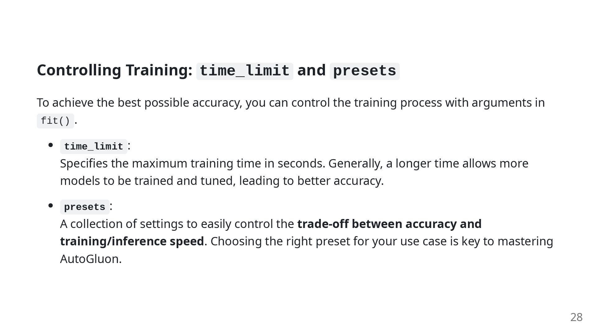
accuracy, you can control the training process with arguments in fit() . time_limit : Specifies the maximum training time in seconds. Generally, a longer time allows more models to be trained and tuned, leading to better accuracy. presets : A collection of settings to easily control the trade-off between accuracy and training/inference speed. Choosing the right preset for your use case is key to mastering AutoGluon. 28
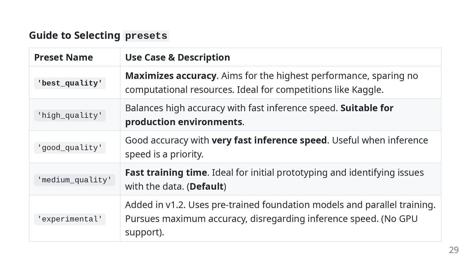
'best_quality' Maximizes accuracy. Aims for the highest performance, sparing no computational resources. Ideal for competitions like Kaggle. 'high_quality' Balances high accuracy with fast inference speed. Suitable for production environments. 'good_quality' Good accuracy with very fast inference speed. Useful when inference speed is a priority. 'medium_quality' Fast training time. Ideal for initial prototyping and identifying issues with the data. (Default) 'experimental' Added in v1.2. Uses pre-trained foundation models and parallel training. Pursues maximum accuracy, disregarding inference speed. (No GPU support). 29
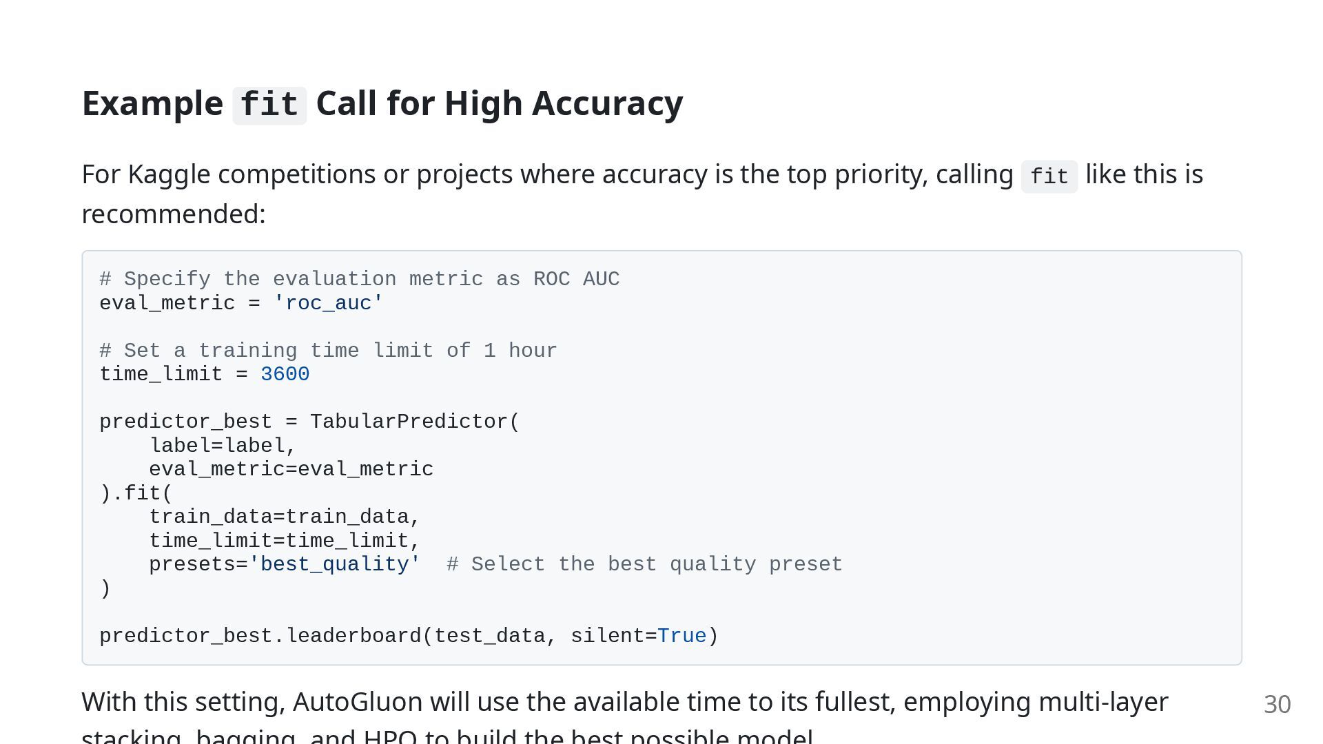
projects where accuracy is the top priority, calling fit like this is recommended: # Specify the evaluation metric as ROC AUC eval_metric = 'roc_auc' # Set a training time limit of 1 hour time_limit = 3600 predictor_best = TabularPredictor( label=label, eval_metric=eval_metric ).fit( train_data=train_data, time_limit=time_limit, presets='best_quality' # Select the best quality preset ) predictor_best.leaderboard(test_data, silent=True) With this setting, AutoGluon will use the available time to its fullest, employing multi-layer 30
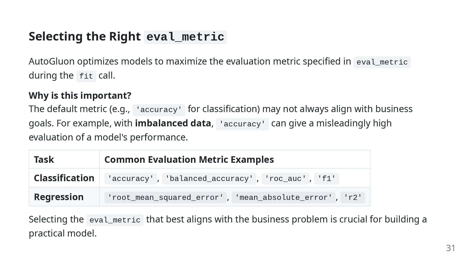
evaluation metric specified in eval_metric during the fit call. Why is this important? The default metric (e.g., 'accuracy' for classification) may not always align with business goals. For example, with imbalanced data, 'accuracy' can give a misleadingly high evaluation of a model's performance. Task Common Evaluation Metric Examples Classification 'accuracy' , 'balanced_accuracy' , 'roc_auc' , 'f1' Regression 'root_mean_squared_error' , 'mean_absolute_error' , 'r2' Selecting the eval_metric that best aligns with the business problem is crucial for building a practical model. 31
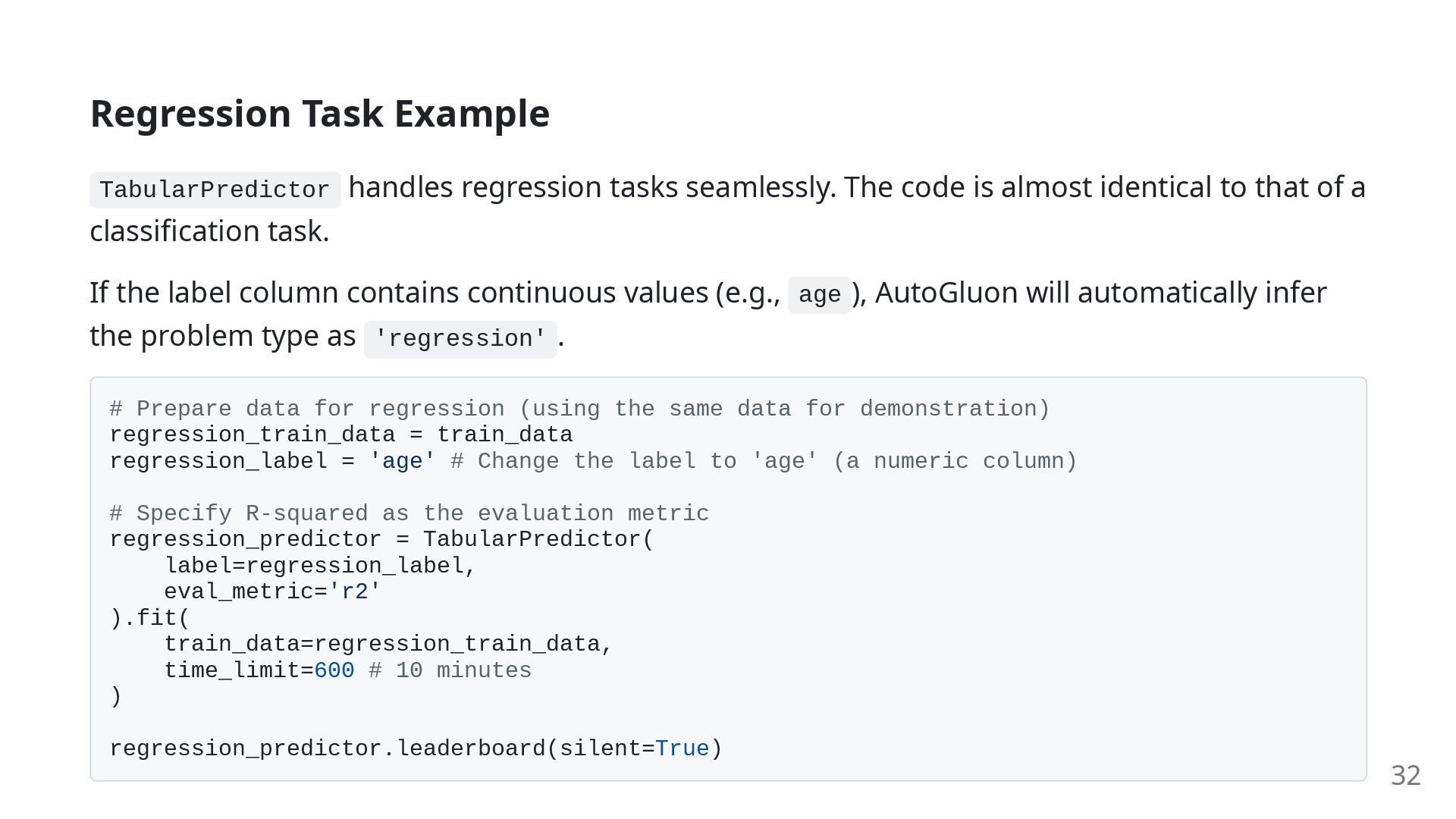
is almost identical to that of a classification task. If the label column contains continuous values (e.g., age ), AutoGluon will automatically infer the problem type as 'regression' . # Prepare data for regression (using the same data for demonstration) regression_train_data = train_data regression_label = 'age' # Change the label to 'age' (a numeric column) # Specify R-squared as the evaluation metric regression_predictor = TabularPredictor( label=regression_label, eval_metric='r2' ).fit( train_data=regression_train_data, time_limit=600 # 10 minutes ) regression_predictor.leaderboard(silent=True) 32
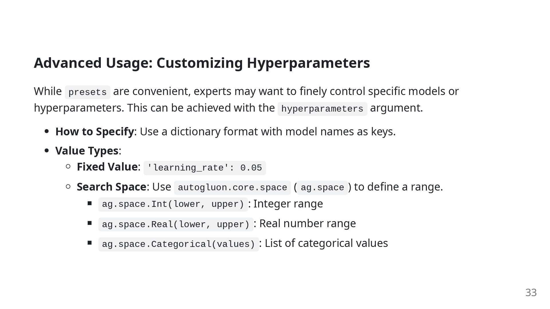
want to finely control specific models or hyperparameters. This can be achieved with the hyperparameters argument. How to Specify: Use a dictionary format with model names as keys. Value Types: Fixed Value: 'learning_rate': 0.05 Search Space: Use autogluon.core.space ( ag.space ) to define a range. ag.space.Int(lower, upper) : Integer range ag.space.Real(lower, upper) : Real number range ag.space.Categorical(values) : List of categorical values 33
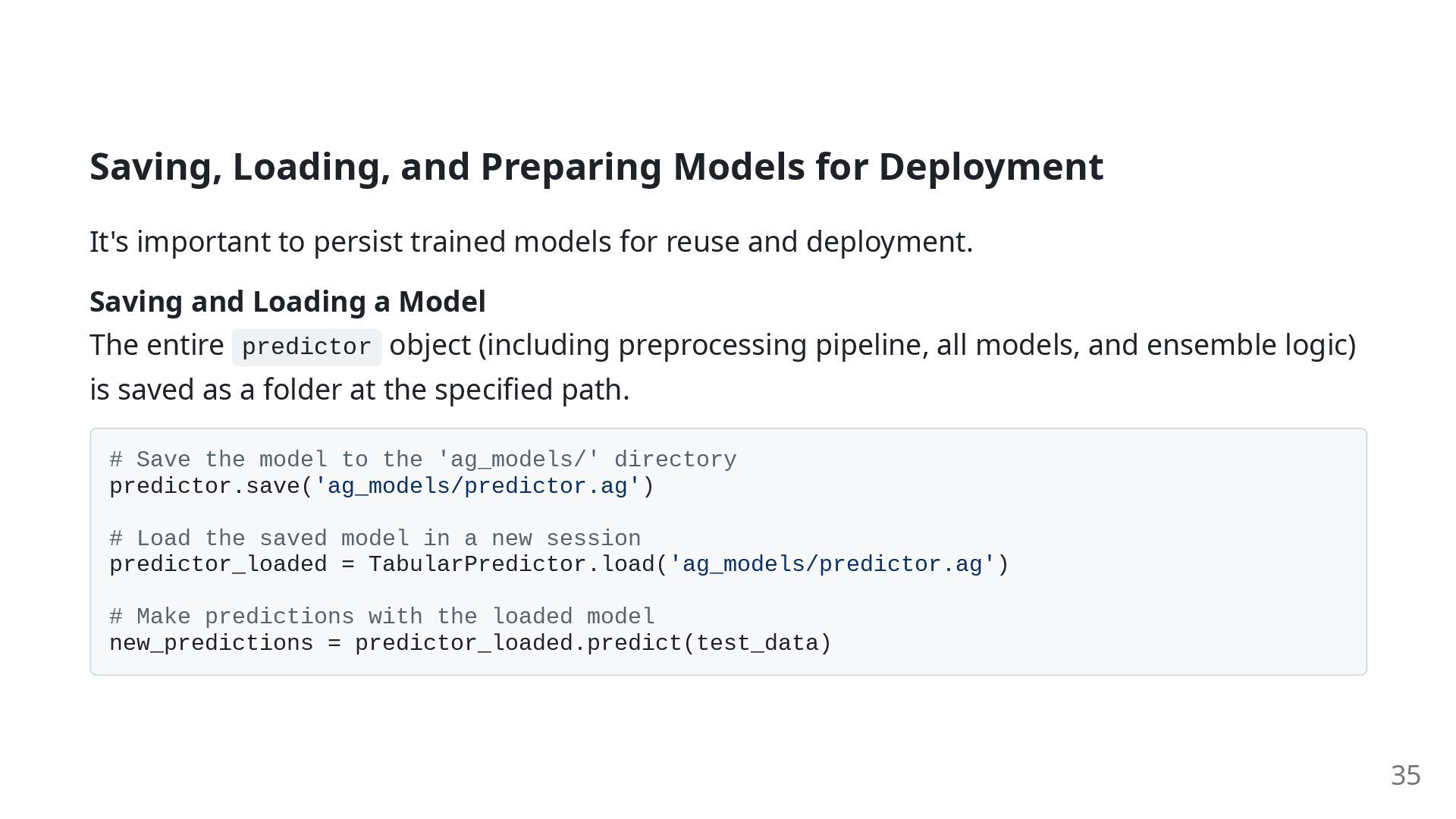
persist trained models for reuse and deployment. Saving and Loading a Model The entire predictor object (including preprocessing pipeline, all models, and ensemble logic) is saved as a folder at the specified path. # Save the model to the 'ag_models/' directory predictor.save('ag_models/predictor.ag') # Load the saved model in a new session predictor_loaded = TabularPredictor.load('ag_models/predictor.ag') # Make predictions with the loaded model new_predictions = predictor_loaded.predict(test_data) 35
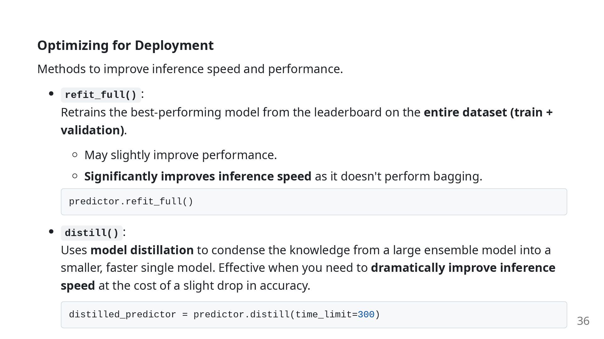
refit_full() : Retrains the best-performing model from the leaderboard on the entire dataset (train + validation). May slightly improve performance. Significantly improves inference speed as it doesn't perform bagging. predictor.refit_full() distill() : Uses model distillation to condense the knowledge from a large ensemble model into a smaller, faster single model. Effective when you need to dramatically improve inference speed at the cost of a slight drop in accuracy. distilled_predictor = predictor.distill(time_limit=300) 36
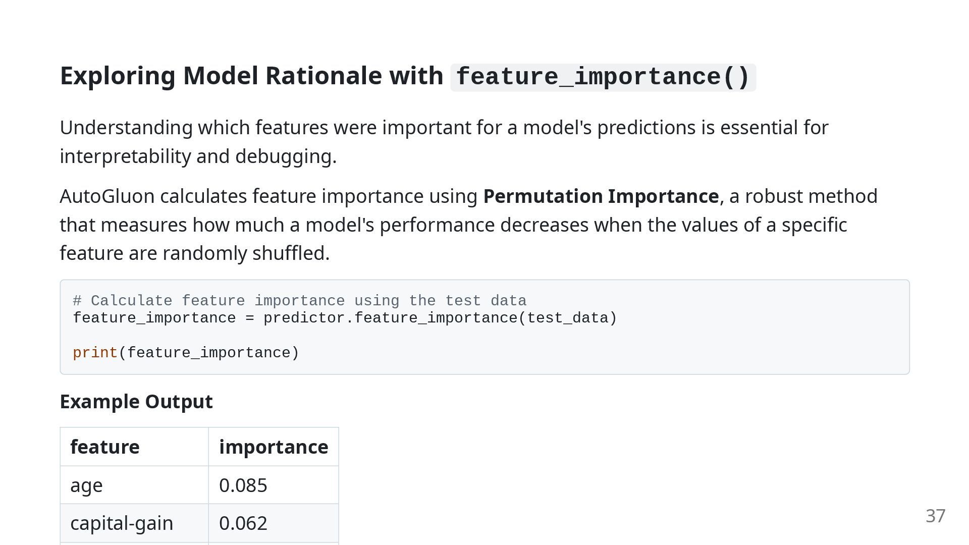
for a model's predictions is essential for interpretability and debugging. AutoGluon calculates feature importance using Permutation Importance, a robust method that measures how much a model's performance decreases when the values of a specific feature are randomly shuffled. # Calculate feature importance using the test data feature_importance = predictor.feature_importance(test_data) print(feature_importance) Example Output feature importance age 0.085 capital-gain 0.062 37
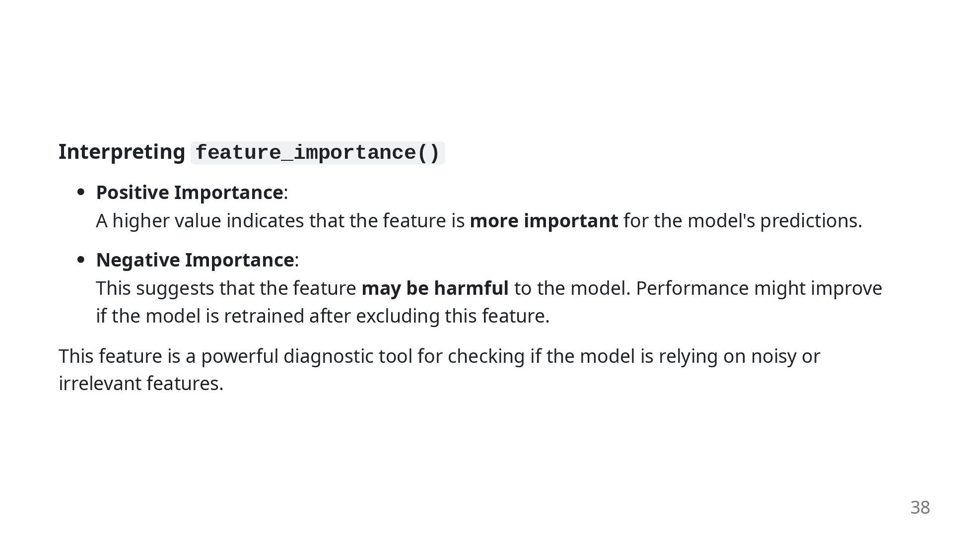
feature is more important for the model's predictions. Negative Importance: This suggests that the feature may be harmful to the model. Performance might improve if the model is retrained after excluding this feature. This feature is a powerful diagnostic tool for checking if the model is relying on noisy or irrelevant features. 38
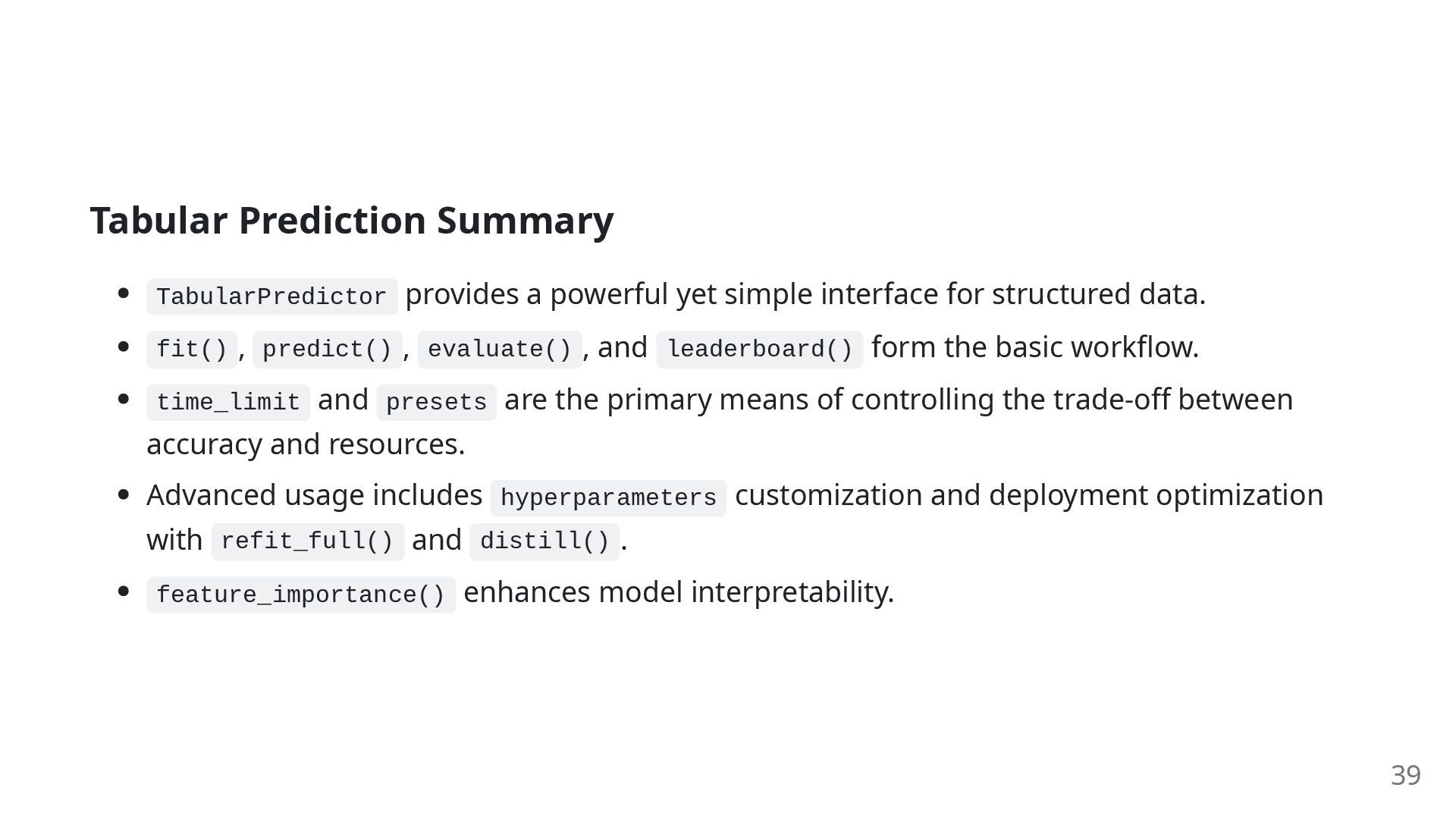
for structured data. fit() , predict() , evaluate() , and leaderboard() form the basic workflow. time_limit and presets are the primary means of controlling the trade-off between accuracy and resources. Advanced usage includes hyperparameters customization and deployment optimization with refit_full() and distill() . feature_importance() enhances model interpretability. 39
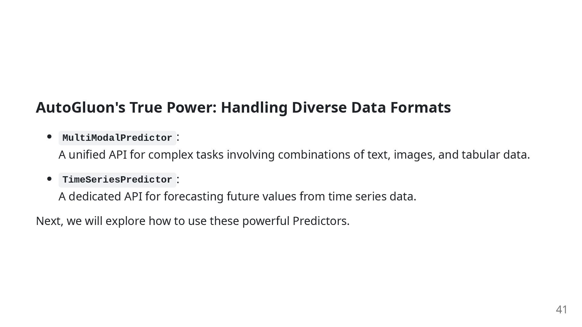
unified API for complex tasks involving combinations of text, images, and tabular data. TimeSeriesPredictor : A dedicated API for forecasting future values from time series data. Next, we will explore how to use these powerful Predictors. 41
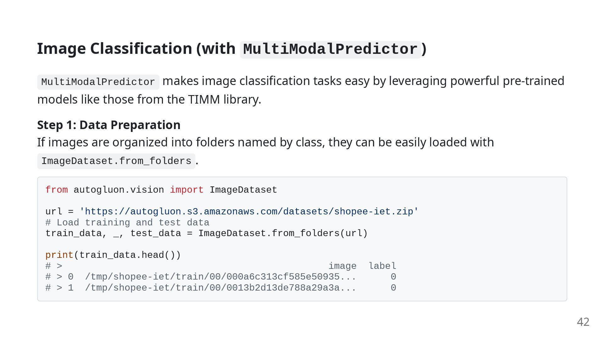
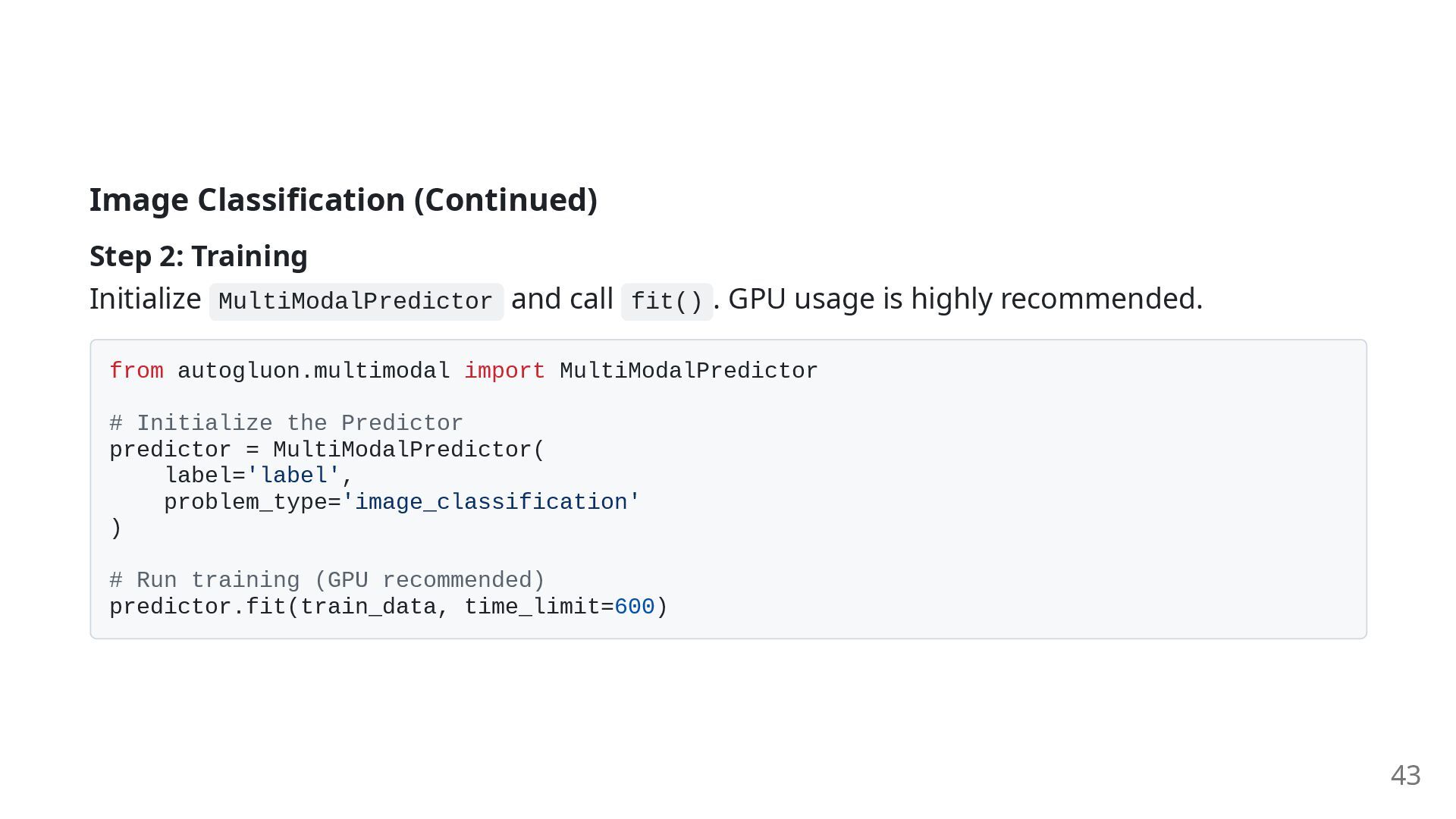
easy by leveraging powerful pre-trained models like those from the TIMM library. Step 1: Data Preparation If images are organized into folders named by class, they can be easily loaded with ImageDataset.from_folders . from autogluon.vision import ImageDataset url = 'https://autogluon.s3.amazonaws.com/datasets/shopee-iet.zip' # Load training and test data train_data, _, test_data = ImageDataset.from_folders(url) print(train_data.head()) # > image label # > 0 /tmp/shopee-iet/train/00/000a6c313cf585e50935... 0 # > 1 /tmp/shopee-iet/train/00/0013b2d13de788a29a3a... 0 42
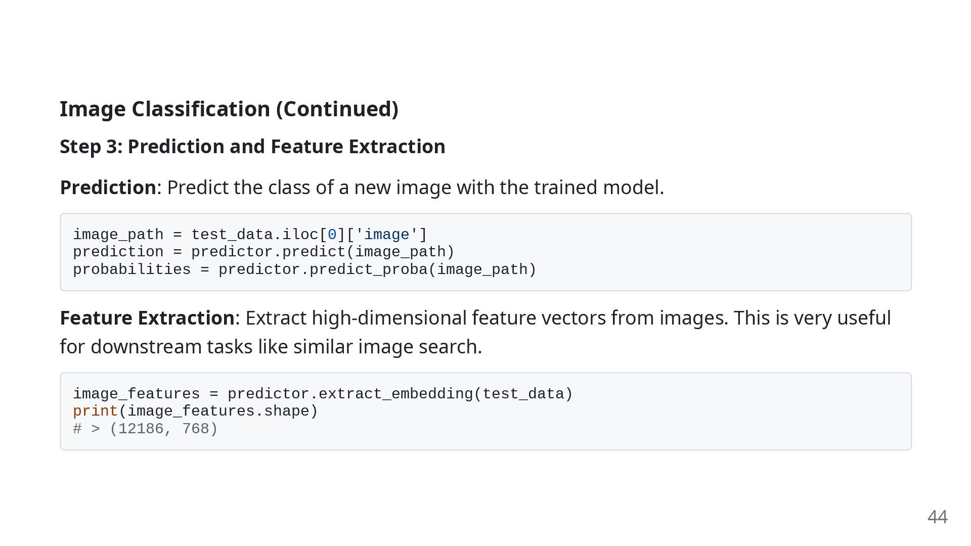
Predict the class of a new image with the trained model. image_path = test_data.iloc[0]['image'] prediction = predictor.predict(image_path) probabilities = predictor.predict_proba(image_path) Feature Extraction: Extract high-dimensional feature vectors from images. This is very useful for downstream tasks like similar image search. image_features = predictor.extract_embedding(test_data) print(image_features.shape) # > (12186, 768) 44
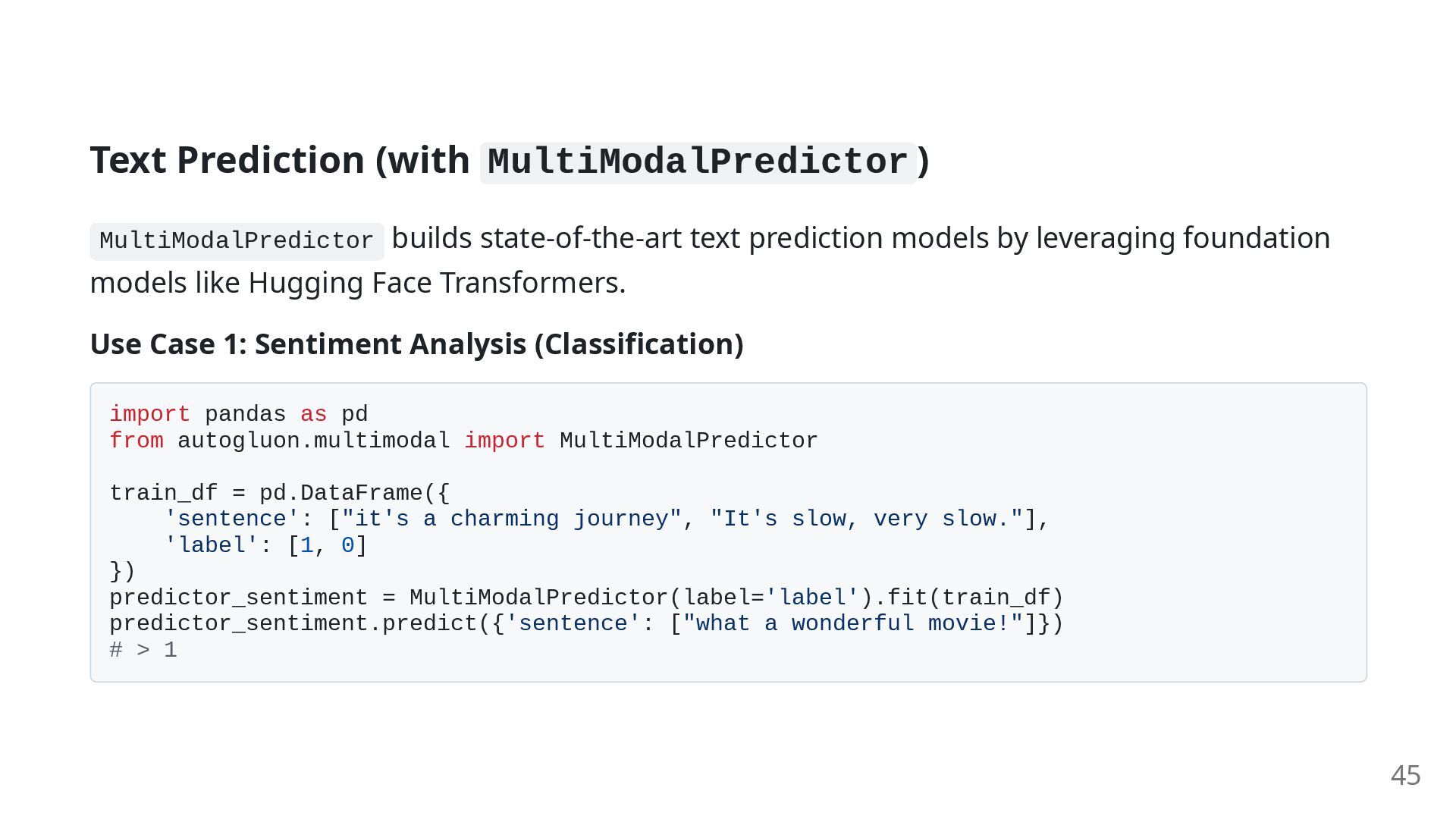
models by leveraging foundation models like Hugging Face Transformers. Use Case 1: Sentiment Analysis (Classification) import pandas as pd from autogluon.multimodal import MultiModalPredictor train_df = pd.DataFrame({ 'sentence': ["it's a charming journey", "It's slow, very slow."], 'label': [1, 0] }) predictor_sentiment = MultiModalPredictor(label='label').fit(train_df) predictor_sentiment.predict({'sentence': ["what a wonderful movie!"]}) # > 1 45
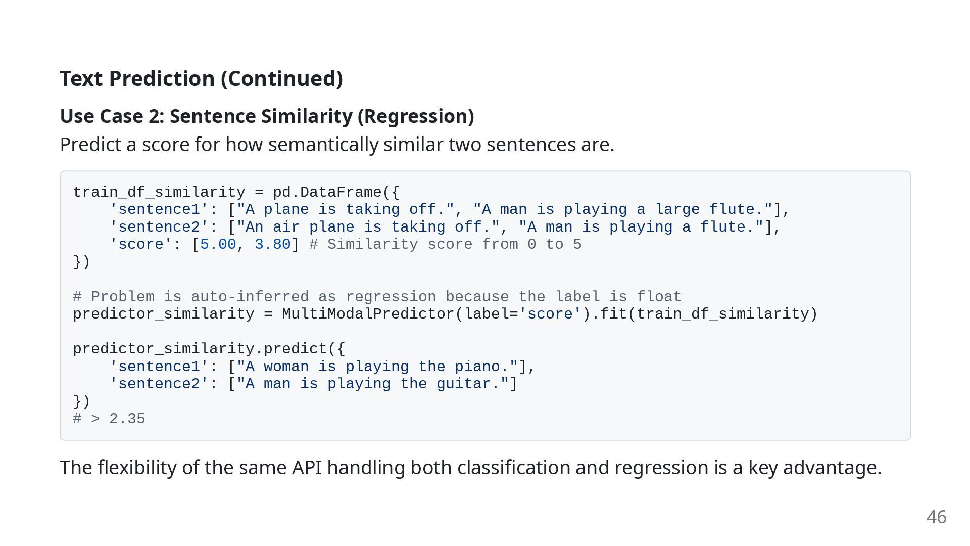
a score for how semantically similar two sentences are. train_df_similarity = pd.DataFrame({ 'sentence1': ["A plane is taking off.", "A man is playing a large flute."], 'sentence2': ["An air plane is taking off.", "A man is playing a flute."], 'score': [5.00, 3.80] # Similarity score from 0 to 5 }) # Problem is auto-inferred as regression because the label is float predictor_similarity = MultiModalPredictor(label='score').fit(train_df_similarity) predictor_similarity.predict({ 'sentence1': ["A woman is playing the piano."], 'sentence2': ["A man is playing the guitar."] }) # > 2.35 The flexibility of the same API handling both classification and regression is a key advantage. 46
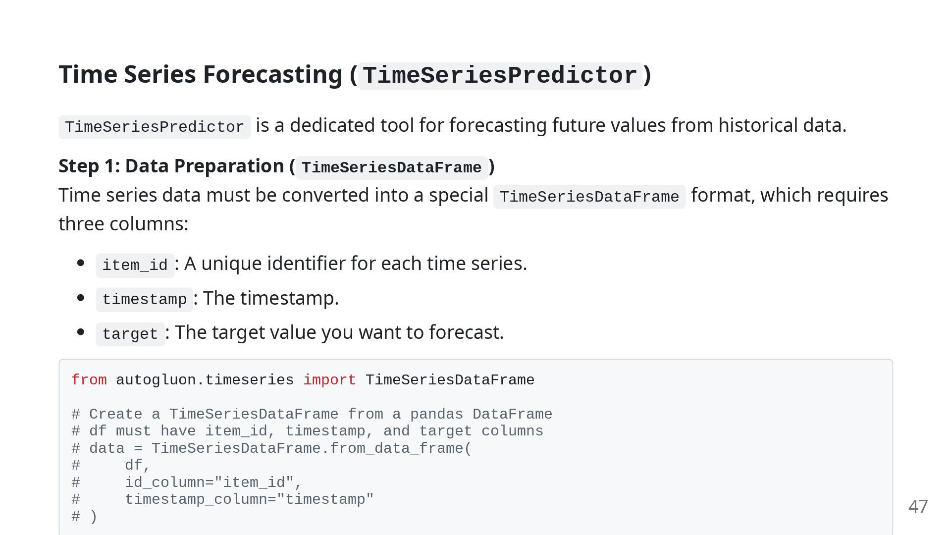
tool for forecasting future values from historical data. Step 1: Data Preparation ( TimeSeriesDataFrame ) Time series data must be converted into a special TimeSeriesDataFrame format, which requires three columns: item_id : A unique identifier for each time series. timestamp : The timestamp. target : The target value you want to forecast. from autogluon.timeseries import TimeSeriesDataFrame # Create a TimeSeriesDataFrame from a pandas DataFrame # df must have item_id, timestamp, and target columns # data = TimeSeriesDataFrame.from_data_frame( # df, # id_column="item_id", # timestamp_column="timestamp" # ) 47
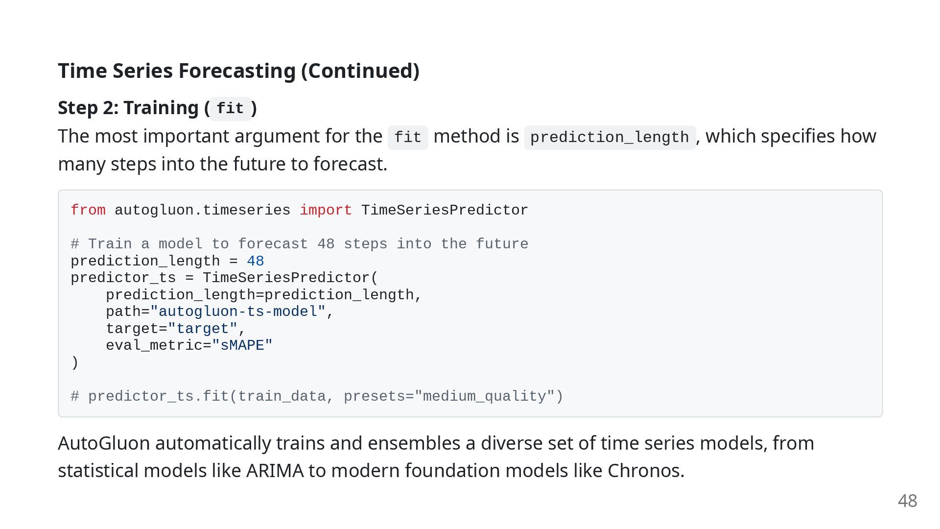
The most important argument for the fit method is prediction_length , which specifies how many steps into the future to forecast. from autogluon.timeseries import TimeSeriesPredictor # Train a model to forecast 48 steps into the future prediction_length = 48 predictor_ts = TimeSeriesPredictor( prediction_length=prediction_length, path="autogluon-ts-model", target="target", eval_metric="sMAPE" ) # predictor_ts.fit(train_data, presets="medium_quality") AutoGluon automatically trains and ensembles a diverse set of time series models, from statistical models like ARIMA to modern foundation models like Chronos. 48
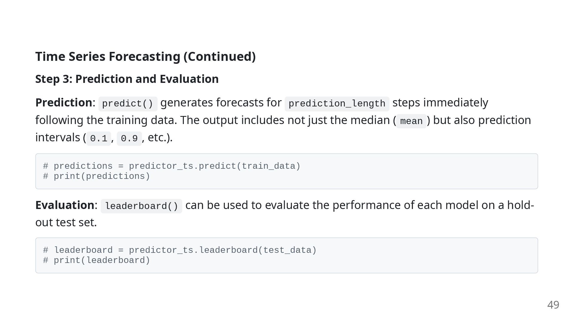
predict() generates forecasts for prediction_length steps immediately following the training data. The output includes not just the median ( mean ) but also prediction intervals ( 0.1 , 0.9 , etc.). # predictions = predictor_ts.predict(train_data) # print(predictions) Evaluation: leaderboard() can be used to evaluate the performance of each model on a hold- out test set. # leaderboard = predictor_ts.leaderboard(test_data) # print(leaderboard) 49
demonstrated in its ability to build predictive models that combine tabular, text, and image data. We'll illustrate this using the PetFinder dataset (predicting pet adoption speed). What to learn from this example: The user's main job becomes data preparation and metadata definition, not model building. By correctly describing the data, you can unlock the full potential of a highly complex and powerful automation pipeline. 50
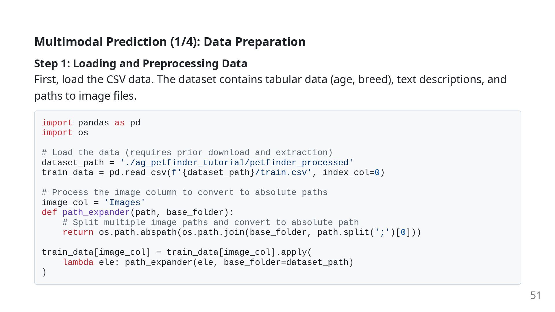
Data First, load the CSV data. The dataset contains tabular data (age, breed), text descriptions, and paths to image files. import pandas as pd import os # Load the data (requires prior download and extraction) dataset_path = './ag_petfinder_tutorial/petfinder_processed' train_data = pd.read_csv(f'{dataset_path}/train.csv', index_col=0) # Process the image column to convert to absolute paths image_col = 'Images' def path_expander(path, base_folder): # Split multiple image paths and convert to absolute path return os.path.abspath(os.path.join(base_folder, path.split(';')[0])) train_data[image_col] = train_data[image_col].apply( lambda ele: path_expander(ele, base_folder=dataset_path) ) 51
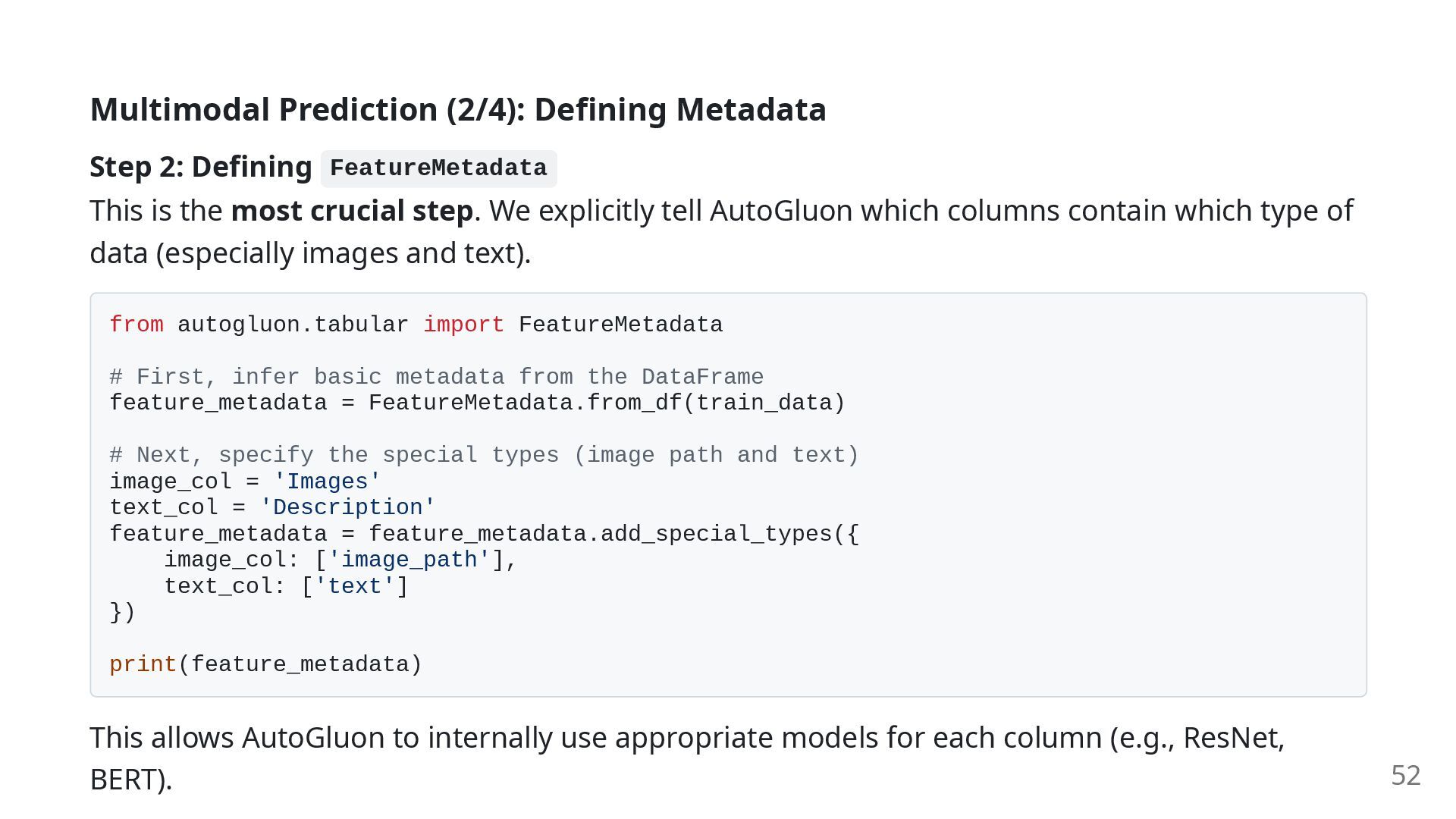
is the most crucial step. We explicitly tell AutoGluon which columns contain which type of data (especially images and text). from autogluon.tabular import FeatureMetadata # First, infer basic metadata from the DataFrame feature_metadata = FeatureMetadata.from_df(train_data) # Next, specify the special types (image path and text) image_col = 'Images' text_col = 'Description' feature_metadata = feature_metadata.add_special_types({ image_col: ['image_path'], text_col: ['text'] }) print(feature_metadata) This allows AutoGluon to internally use appropriate models for each column (e.g., ResNet, BERT). 52
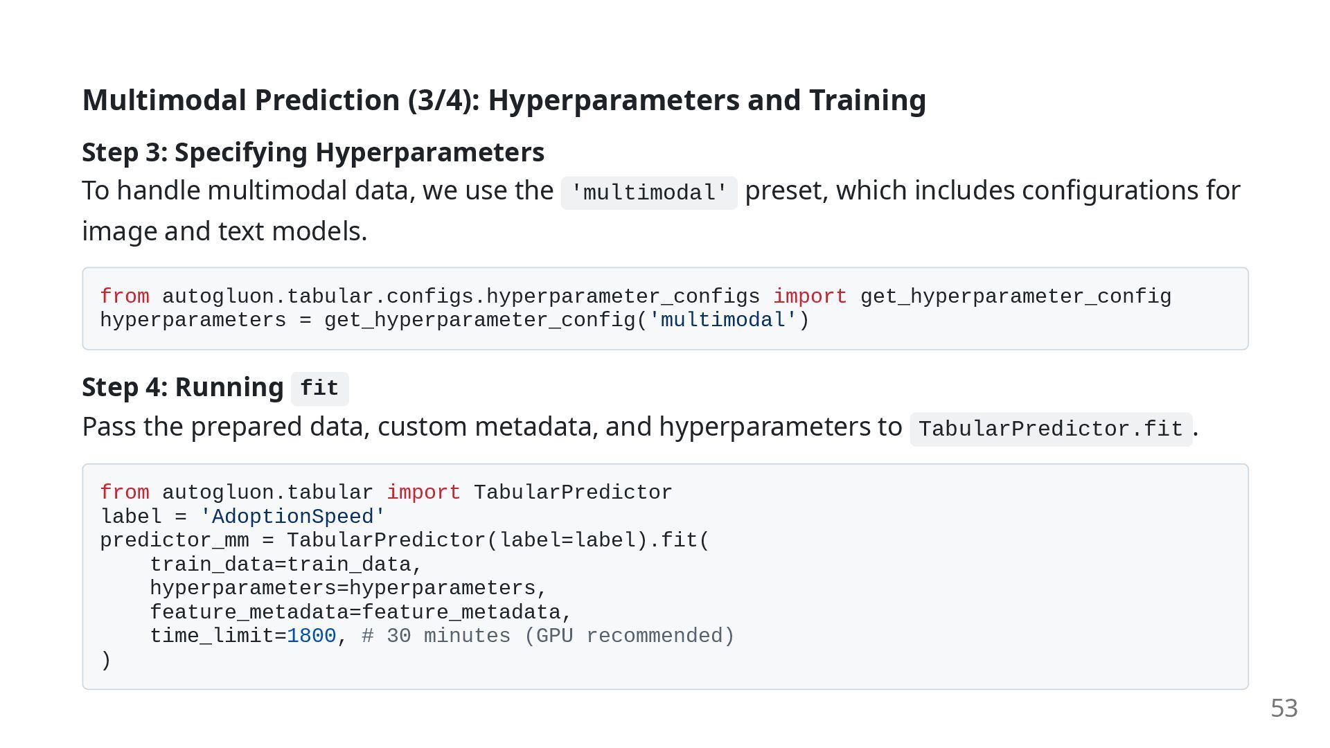
To handle multimodal data, we use the 'multimodal' preset, which includes configurations for image and text models. from autogluon.tabular.configs.hyperparameter_configs import get_hyperparameter_config hyperparameters = get_hyperparameter_config('multimodal') Step 4: Running fit Pass the prepared data, custom metadata, and hyperparameters to TabularPredictor.fit . from autogluon.tabular import TabularPredictor label = 'AdoptionSpeed' predictor_mm = TabularPredictor(label=label).fit( train_data=train_data, hyperparameters=hyperparameters, feature_metadata=feature_metadata, time_limit=1800, # 30 minutes (GPU recommended) ) 53
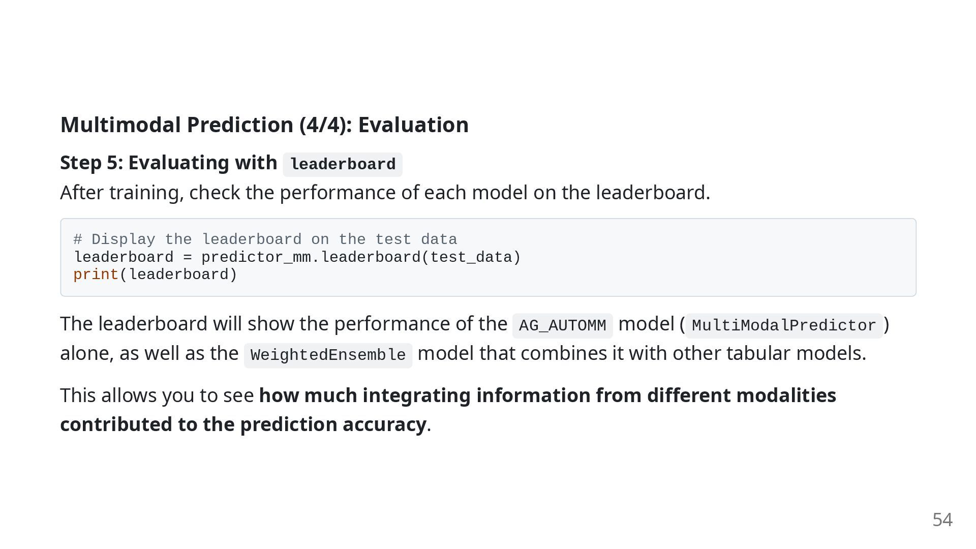
training, check the performance of each model on the leaderboard. # Display the leaderboard on the test data leaderboard = predictor_mm.leaderboard(test_data) print(leaderboard) The leaderboard will show the performance of the AG_AUTOMM model ( MultiModalPredictor ) alone, as well as the WeightedEnsemble model that combines it with other tabular models. This allows you to see how much integrating information from different modalities contributed to the prediction accuracy. 54
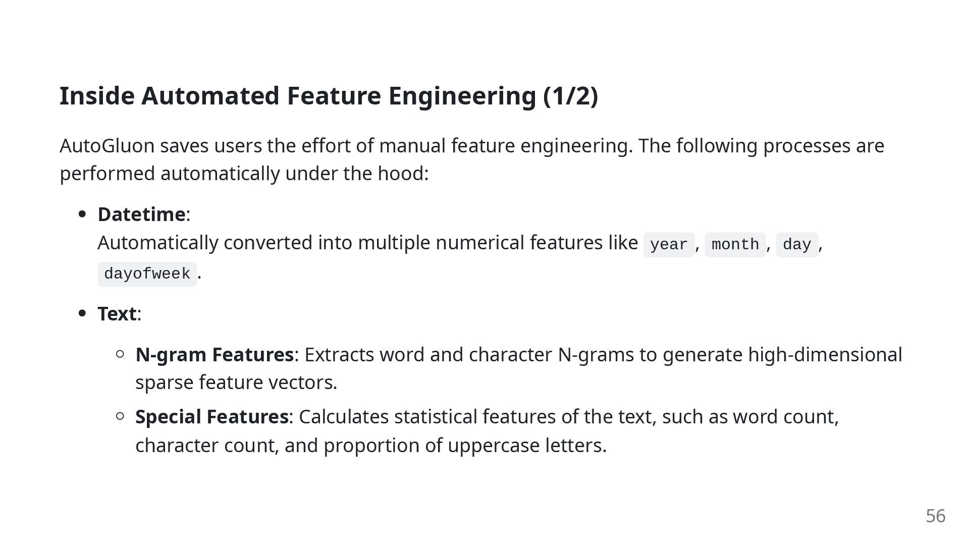
of manual feature engineering. The following processes are performed automatically under the hood: Datetime: Automatically converted into multiple numerical features like year , month , day , dayofweek . Text: N-gram Features: Extracts word and character N-grams to generate high-dimensional sparse feature vectors. Special Features: Calculates statistical features of the text, such as word count, character count, and proportion of uppercase letters. 56
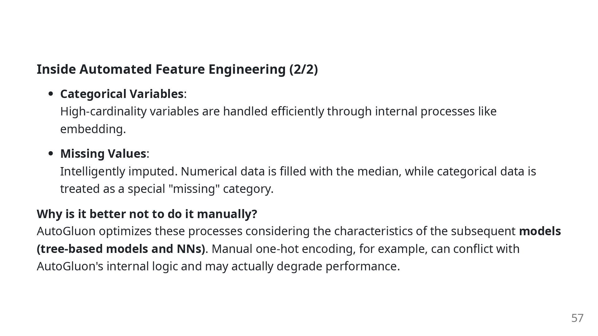
handled efficiently through internal processes like embedding. Missing Values: Intelligently imputed. Numerical data is filled with the median, while categorical data is treated as a special "missing" category. Why is it better not to do it manually? AutoGluon optimizes these processes considering the characteristics of the subsequent models (tree-based models and NNs). Manual one-hot encoding, for example, can conflict with AutoGluon's internal logic and may actually degrade performance. 57
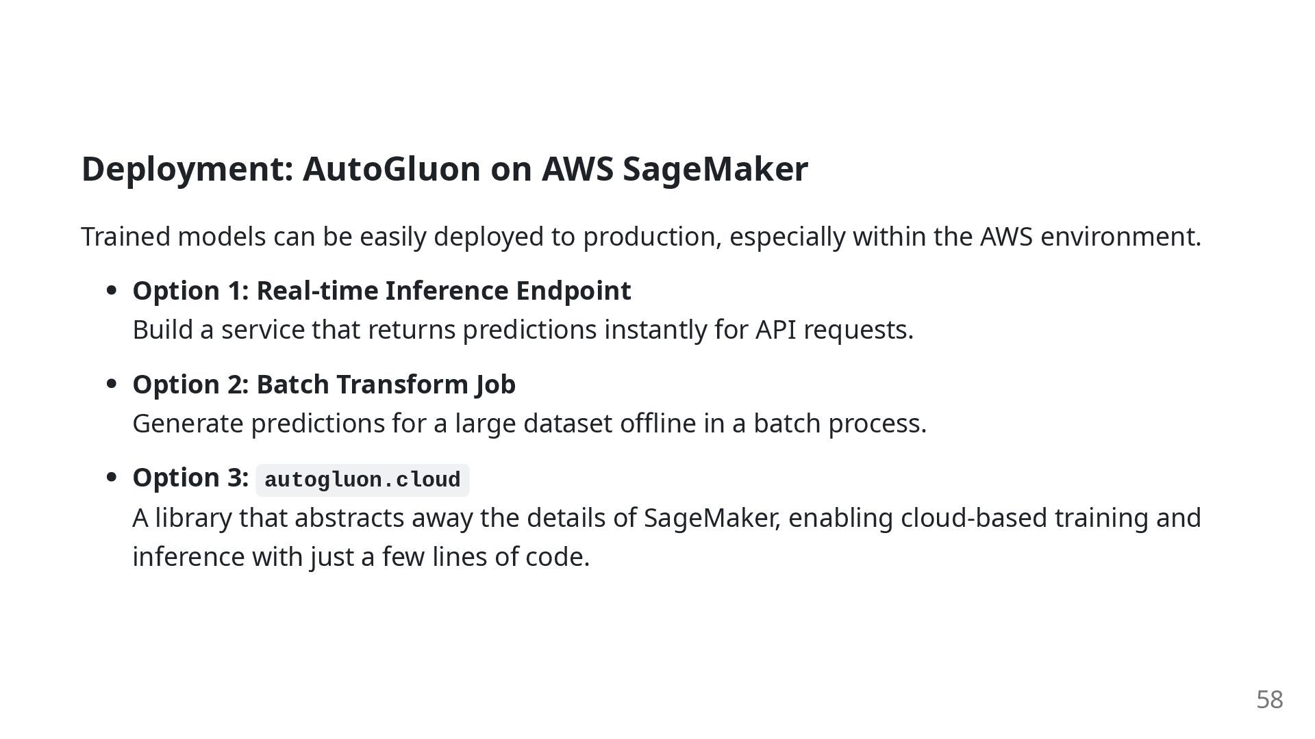
deployed to production, especially within the AWS environment. Option 1: Real-time Inference Endpoint Build a service that returns predictions instantly for API requests. Option 2: Batch Transform Job Generate predictions for a large dataset offline in a batch process. Option 3: autogluon.cloud A library that abstracts away the details of SageMaker, enabling cloud-based training and inference with just a few lines of code. 58
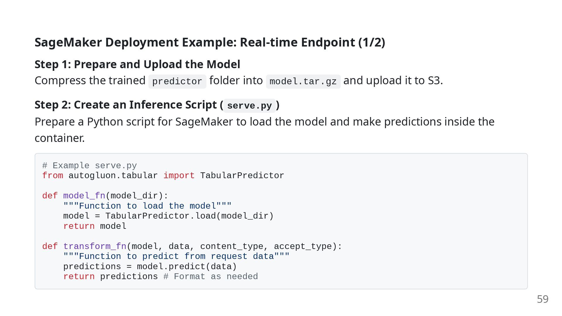
Upload the Model Compress the trained predictor folder into model.tar.gz and upload it to S3. Step 2: Create an Inference Script ( serve.py ) Prepare a Python script for SageMaker to load the model and make predictions inside the container. # Example serve.py from autogluon.tabular import TabularPredictor def model_fn(model_dir): """Function to load the model""" model = TabularPredictor.load(model_dir) return model def transform_fn(model, data, content_type, accept_type): """Function to predict from request data""" predictions = model.predict(data) return predictions # Format as needed 59
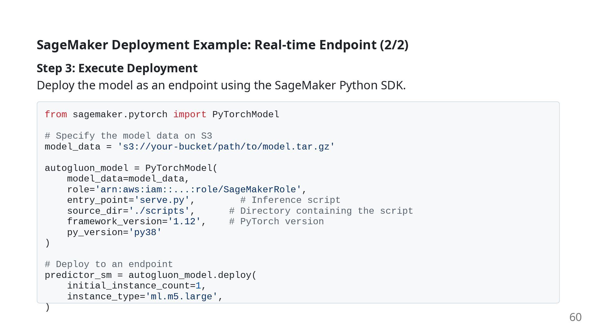
Deploy the model as an endpoint using the SageMaker Python SDK. from sagemaker.pytorch import PyTorchModel # Specify the model data on S3 model_data = 's3://your-bucket/path/to/model.tar.gz' autogluon_model = PyTorchModel( model_data=model_data, role='arn:aws:iam::...:role/SageMakerRole', entry_point='serve.py', # Inference script source_dir='./scripts', # Directory containing the script framework_version='1.12', # PyTorch version py_version='py38' ) # Deploy to an endpoint predictor_sm = autogluon_model.deploy( initial_instance_count=1, instance_type='ml.m5.large', ) 60
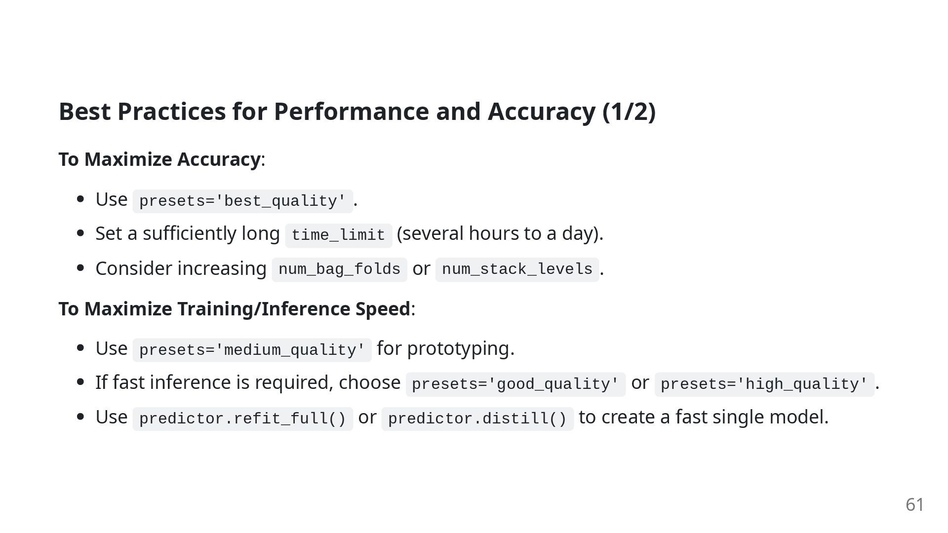
Use presets='best_quality' . Set a sufficiently long time_limit (several hours to a day). Consider increasing num_bag_folds or num_stack_levels . To Maximize Training/Inference Speed: Use presets='medium_quality' for prototyping. If fast inference is required, choose presets='good_quality' or presets='high_quality' . Use predictor.refit_full() or predictor.distill() to create a fast single model. 61
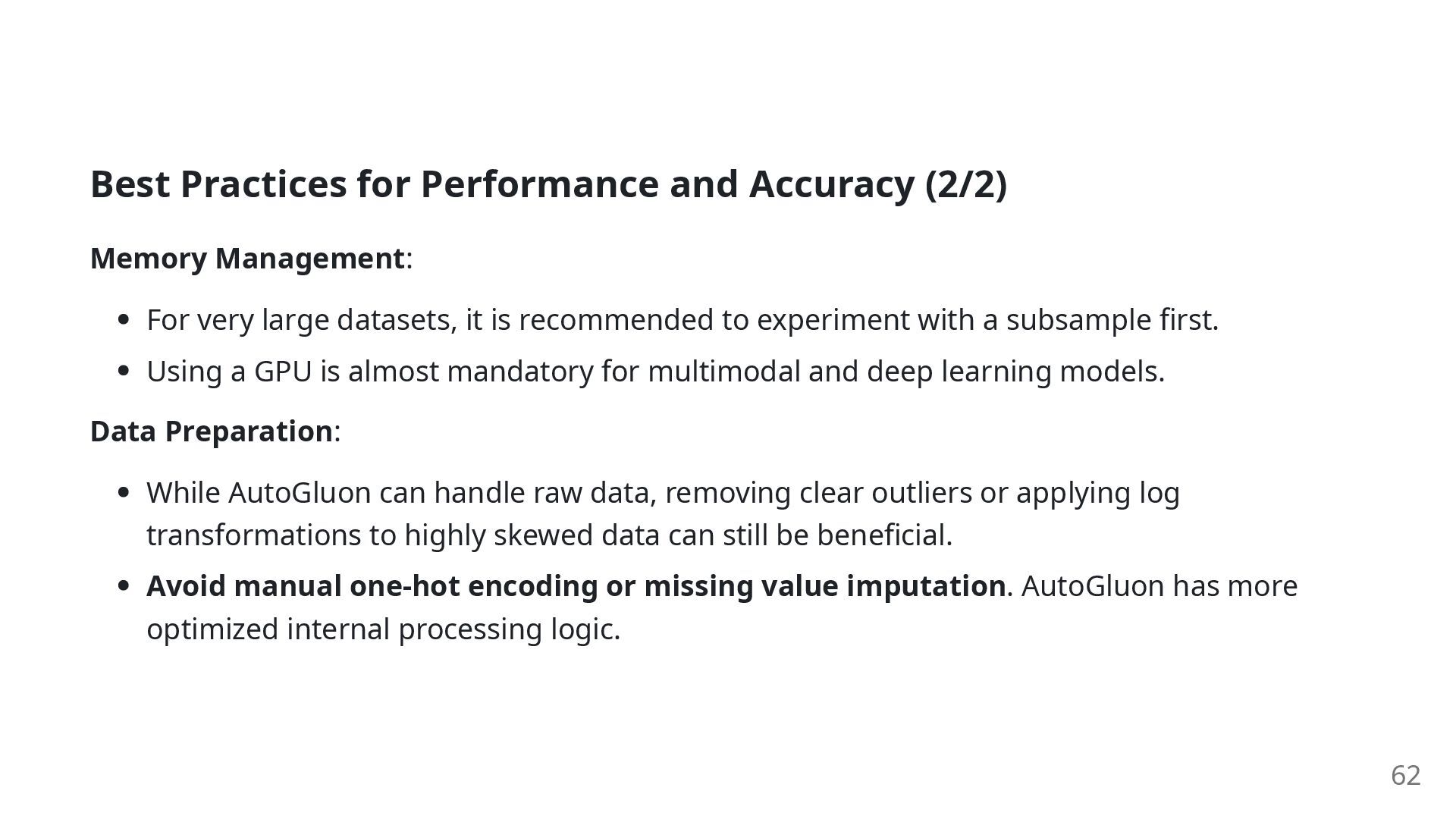
very large datasets, it is recommended to experiment with a subsample first. Using a GPU is almost mandatory for multimodal and deep learning models. Data Preparation: While AutoGluon can handle raw data, removing clear outliers or applying log transformations to highly skewed data can still be beneficial. Avoid manual one-hot encoding or missing value imputation. AutoGluon has more optimized internal processing logic. 62
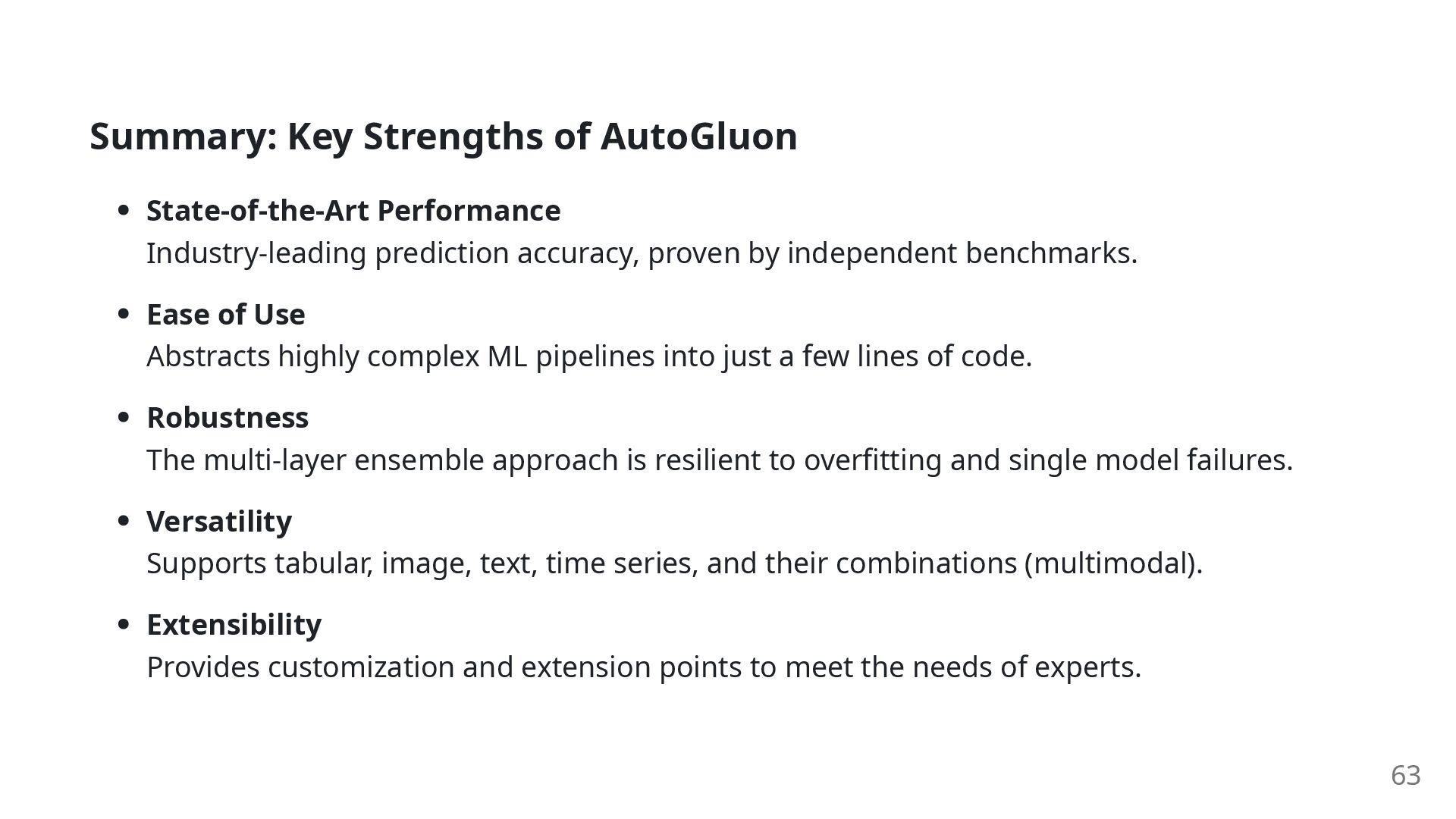
proven by independent benchmarks. Ease of Use Abstracts highly complex ML pipelines into just a few lines of code. Robustness The multi-layer ensemble approach is resilient to overfitting and single model failures. Versatility Supports tabular, image, text, time series, and their combinations (multimodal). Extensibility Provides customization and extension points to meet the needs of experts. 63
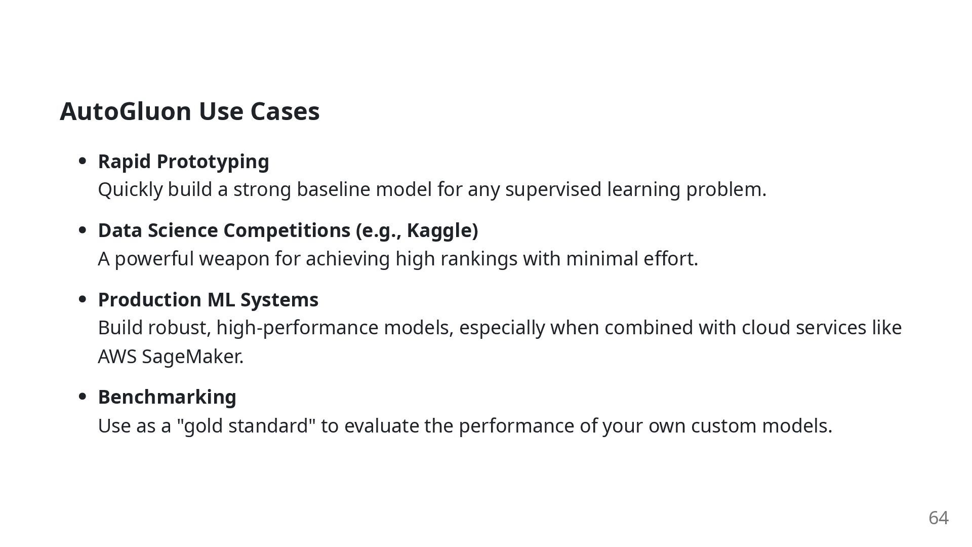
model for any supervised learning problem. Data Science Competitions (e.g., Kaggle) A powerful weapon for achieving high rankings with minimal effort. Production ML Systems Build robust, high-performance models, especially when combined with cloud services like AWS SageMaker. Benchmarking Use as a "gold standard" to evaluate the performance of your own custom models. 64
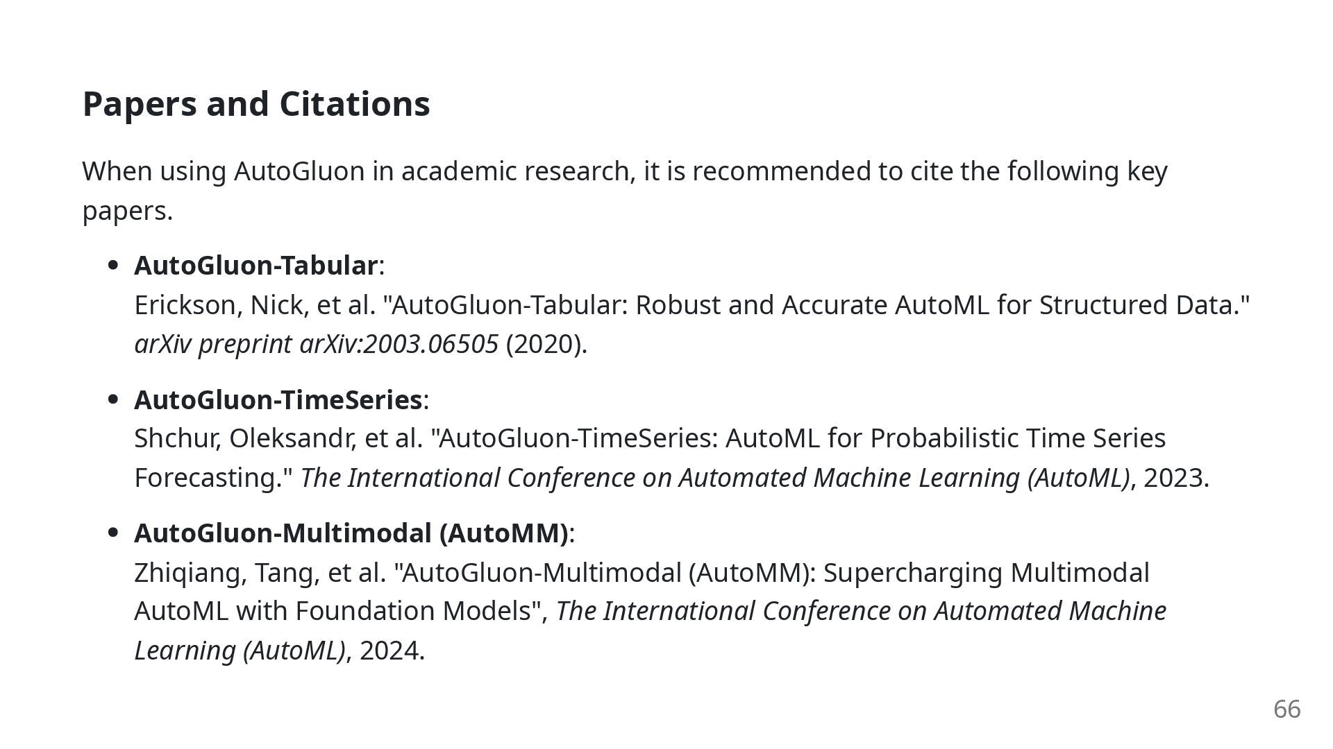
is recommended to cite the following key papers. AutoGluon-Tabular: Erickson, Nick, et al. "AutoGluon-Tabular: Robust and Accurate AutoML for Structured Data." arXiv preprint arXiv:2003.06505 (2020). AutoGluon-TimeSeries: Shchur, Oleksandr, et al. "AutoGluon-TimeSeries: AutoML for Probabilistic Time Series Forecasting." The International Conference on Automated Machine Learning (AutoML), 2023. AutoGluon-Multimodal (AutoMM): Zhiqiang, Tang, et al. "AutoGluon-Multimodal (AutoMM): Supercharging Multimodal AutoML with Foundation Models", The International Conference on Automated Machine Learning (AutoML), 2024. 66