bayesImageS: an R package for Bayesian image analysis

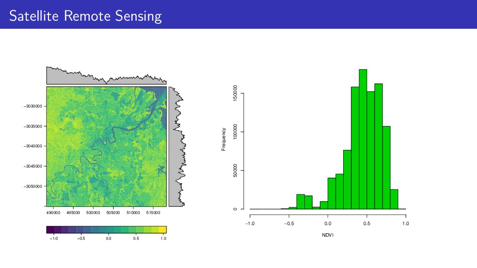
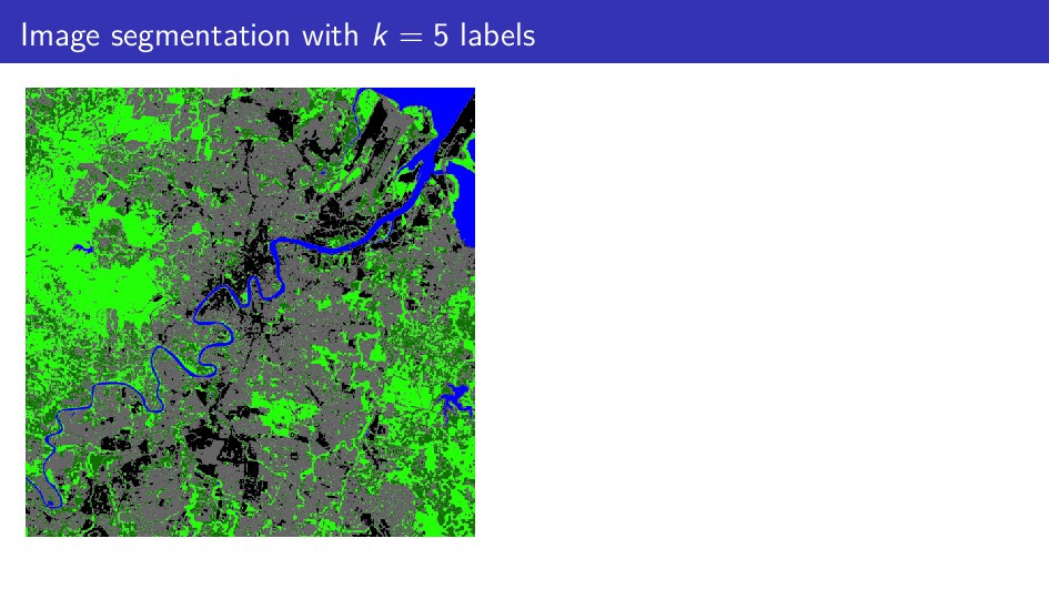
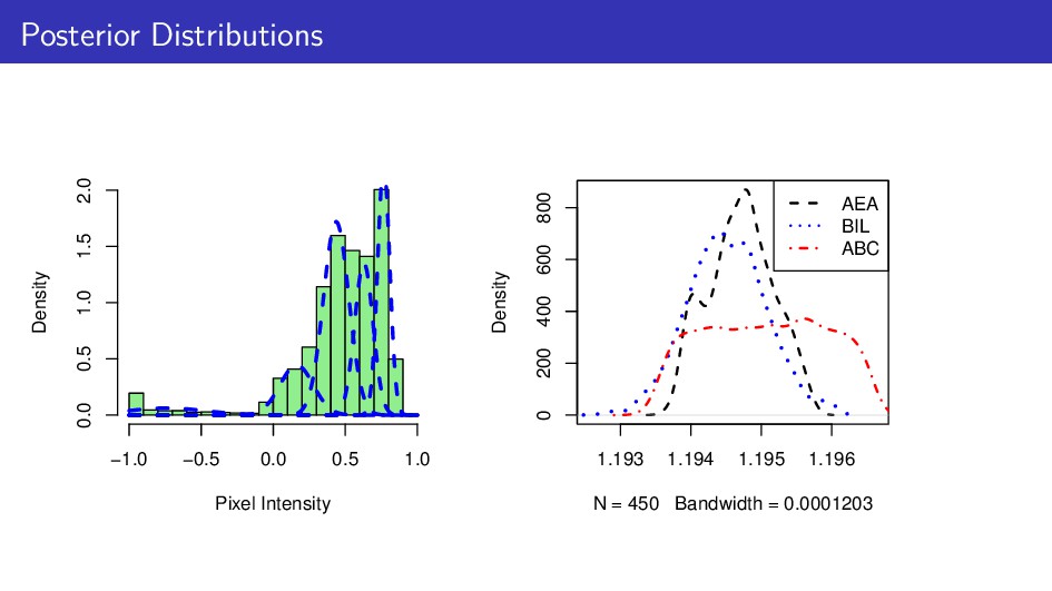
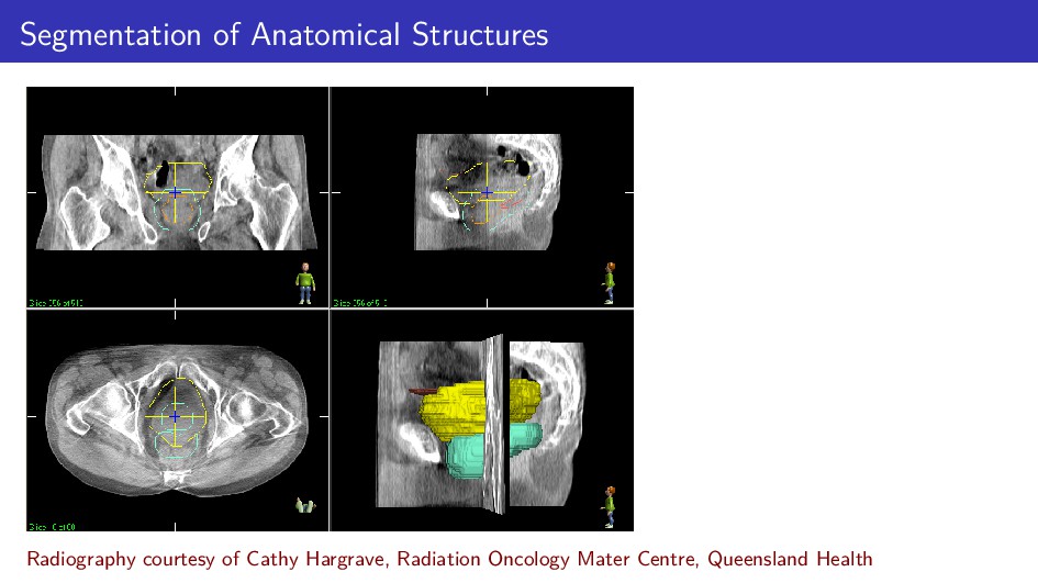
There are many approaches to Bayesian computation with intractable likelihoods, including the exchange algorithm, approximate Bayesian computation (ABC), thermodynamic integration, and composite likelihood. These approaches vary in accuracy as well as scalability for datasets of significant size. The Potts model is an example where such methods are required, due to its intractable normalising constant. This model is a type of Markov random field, which is commonly used for image segmentation. The dimension of its parameter space increases linearly with the number of pixels in the image, making this a challenging application for scalable Bayesian computation. My talk will introduce various algorithms in the context of the Potts model and describe their implementation in C++, using OpenMP for parallelism. I will also discuss the process of releasing this software as an open source R package on the CRAN repository.

Transcript

1. bayesImageS: an R package for Bayesian image analysis Matt Moores @MooresMt https://mooresm.github.io/bayesImageS NIASRA, University of Wollongong, NSW, Australia useR! 2018 1 / 22
2. Image Segmentation Classifying the observed pixel intensities y := {yi }n i=1 ∈ Rn according to a set of latent labels z := {zi }n i=1 ∈ [1, . . . , k]n Assuming additive Gaussian noise: yi | zi = j ∼ N µj, σ2 j The resulting augmented likelihood is a mixture of Gaussians: p(y, z | µ, σ2, β) = n i=1 p yi | µzi , σ2 zi p(zi | z\i , β) 2 / 22 Rydén & Titterington (1998) J. Comput. Graph. Stat. 7(2): 194–211.
3. Synthetic Data z <- sample.int(3, 49, TRUE) mu <- c(-1, 0, 1) sigma <- rep(0.3, 3) y <- rnorm(49, mu[z], sigma[z]) 2 4 6 Y −1 0 1 Z 0.0 0.2 0.4 0.6 density Component Means −1 0 1 3 / 22
4. Mixture Model library(bayesImageS) lPriors <- list(k=3, mu=c(-1,0,1), mu.sd=rep(0.25,3), sigma=rep(0.5,3), sigma.nu=rep(5,3), lambda=rep(1,3)) mix.fit <- gibbsGMM(y, priors=lPriors) mu[1] mu[2] mu[3] 0 200 400 600 800 1000 0 200 400 600 800 1000 0 200 400 600 800 1000 0.4 0.8 1.2 1.6 −0.8 −0.4 0.0 0.4 −1.50 −1.25 −1.00 −0.75 −0.50 mu[1] mu[2] mu[3] −1.4 −1.2 −1.0 −0.8 −0.6 −0.4 −0.8 −0.4 0.0 0.4 0.4 0.8 1.2 1.6 Estimated True 4 / 22
5. Pixel Classification Ground Truth Classification 5 / 22
6. Potts model In many images, neighbouring pixels tend to share the same label. This tendency can be represented using a hidden Markov random field: p(zi | z\i , β) = exp{β i∼ δ(zi , z )} k j=1 exp{β i∼ δ(j, z )} where: β is the inverse temperature parameter, i ∼ are the neighbours of pixel i, and δ(x, y) is the Kronecker delta function. 6 / 22 Potts (1952) Proceedings of the Cambridge Philosophical Society 48(1)
7. Inverse Temperature 7 / 22
8. Synthetic Data Using the Swendsen-Wang algorithm to simulate from the Potts model with known β: mask <- matrix(1, nrow=7, ncol=7) neigh <- getNeighbors(mask, c(2,2,0,0)) blocks <- getBlocks(mask, 2) k <- 3 beta <- 0.88 res.sw <- swNoData(beta, k, neigh, blocks, niter=200) z <- matrix(max.col(res.sw$z)[1:nrow(neigh)], nrow=nrow(mask)) y <- rnorm(49, mu[z], sigma[z]) 8 / 22
9. Fitting the Model lPriors <- list(k=3, mu=c(-1,0,1), mu.sd=rep(0.25,3), sigma=rep(0.5,3), sigma.nu=rep(5,3), beta=c(0,2)) mh <- list(algorithm="ex",bandwidth=0.001,auxiliary=200) mrf.fit <- mcmcPotts(y, neigh, blocks, lPriors, mh, niter=500, nburn=250) 0.0 0.5 1.0 0 100 200 300 400 500 beta beta 0.0 0.5 1.0 Estimated True 9 / 22
10. Pixel Classification Ground Truth Classification 10 / 22
11. Intractable Likelihood p(β|z) = C−1(β)eβS(z)π(β) β C−1(β)eβS(z)π(dβ) (1) The normalising constant has computational complexity O(nkn), since it involves a sum over all possible combinations of the labels z ∈ Z: C(β) = z∈Z eβS(z) (2) S(z) is the sufficient statistic of the Potts model: S(z) = i∼ ∈E δ(zi , z ) (3) where E is the set of all unique neighbour pairs. 11 / 22
12. Algorithms for β The argument mh$alg selects which algorithm to use for sampling from p(β|z): pseudolikelihood path sampling (thermodynamic integration) approximate exchange algorithm (AEA) approximate Bayesian computation (ABC-MCMC and ABC-SMC) Bayesian indirect likelihood (BIL) 12 / 22 Moores, Drovandi, Mengersen & Robert (2015) Stat. Comput. 25(1): 23–33. Moores, Pettitt & Mengersen (2015; v2 2018) arXiv:1503.08066 [stat.CO]
13. Satellite Remote Sensing −3050000 −3045000 −3040000 −3035000 −3030000 490000 495000 500000 505000 510000 515000 −1.0 −0.5 0.0 0.5 1.0 NDVI Frequency −1.0 −0.5 0.0 0.5 1.0 0 50000 100000 150000 13 / 22
14. Image segmentation with k = 5 labels 14 / 22
15. Posterior Distributions Pixel Intensity Density −1.0 −0.5 0.0 0.5 1.0 0.0 0.5 1.0 1.5 2.0 1.193 1.194 1.195 1.196 0 200 400 600 800 N = 450 Bandwidth = 0.0001203 Density AEA BIL ABC 15 / 22
16. Segmentation of Anatomical Structures 16 / 22 Radiography courtesy of Cathy Hargrave, Radiation Oncology Mater Centre, Queensland Health
17. External Field Prior p(zi |zi∼ , β, µ, σ2, yi ) = exp {αi,zi + π(αi,zi )} k j=1 exp {αi,j + π(αi,j)} π(zi |zi∼ , β) (4) Isotropic translation: π(αi,j) = log    1 nj h∈j φ ∆(h, i)|µ∆ = 1.2, σ2 ∆ = 7.32    (5) where nj is the number of voxels in object j h ∈ j are the voxels in object j ∆(u, v) is the Euclidean distance between the coordinates of pixel u and pixel v µ∆, σ2 ∆ are parameters that describe the level of spatial variability of the object j 17 / 22
18. Patient- and Organ-Specific Prior αi (prostate) ∼ MVN       0.1 −0.5 0.2    ,    4.12 0 0 0 2.92 0 0 0 0.92       18 / 22
19. Seminal Vesicles αi (SV) ∼ MVN       1.2 −0.7 −0.9    ,    7.32 0 0 0 4.52 0 0 0 1.92       19 / 22
20. Gaussian Random Field 20 / 22
21. Results −300 −250 −200 −150 150 200 250 300 right−left (mm) posterior−anterior (mm) −300 −250 −200 −150 150 200 250 300 right−left (mm) posterior−anterior (mm) 21 / 22 Moores, Hargrave, Deegan, Poulsen, Harden & Mengersen (2015) CSDA 86: 27–41.
22. Summary bayesImageS can be used for segmentation of 2D and 3D images: Update labels using chequerboard Gibbs sampling or Swendsen-Wang Posterior for β using the exchange algorithm, ABC, pseudolikelihood, path sampling, or BIL Fast implementation using RcppArmadillo Parallelism using OpenMP PkgDown documentation: https://mooresm.github.io/bayesImageS Version 0.5-2 currently available on CRAN: https://CRAN.R-project.org/package=bayesImageS 22 / 22