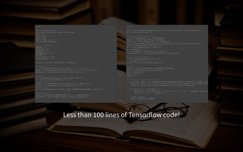
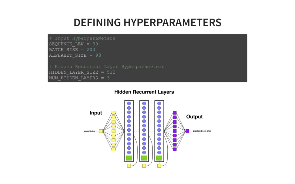
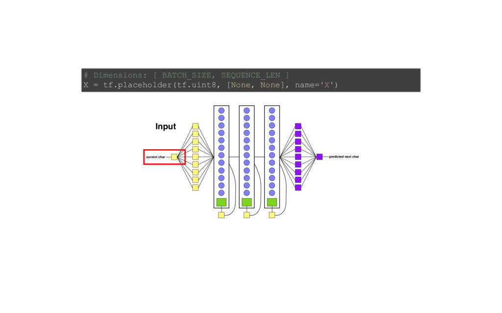
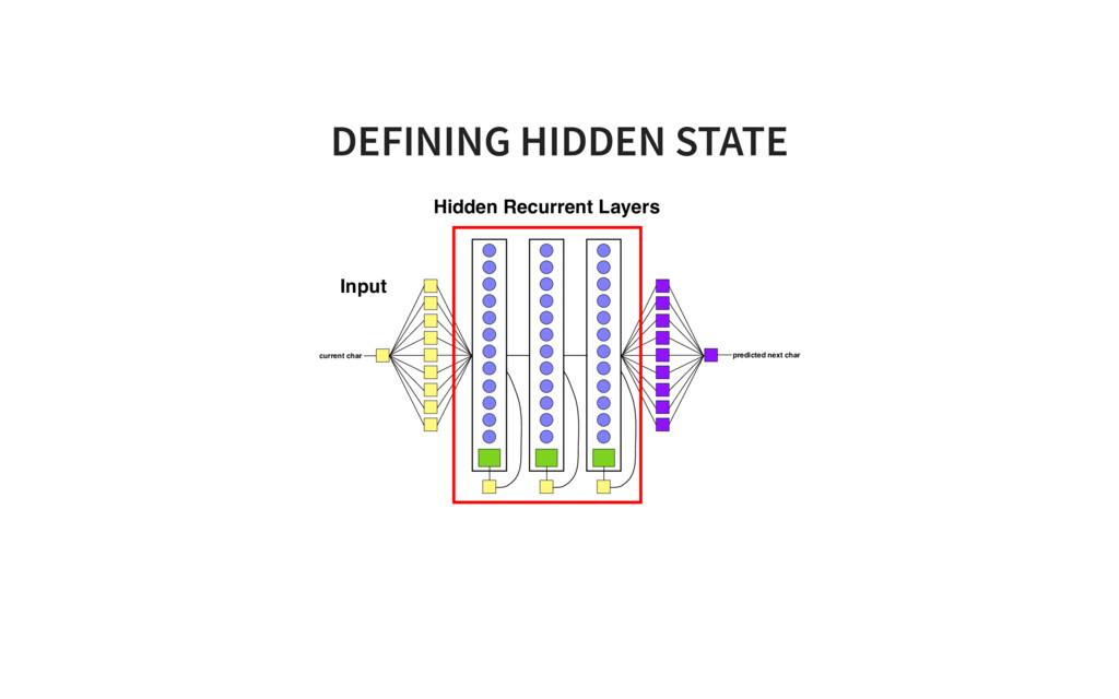
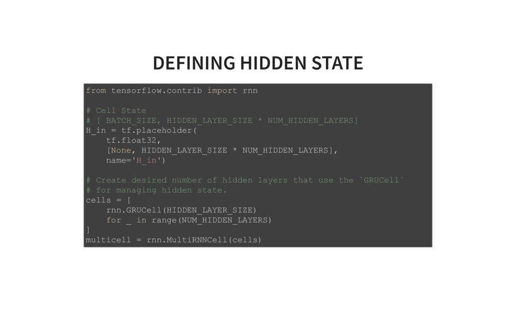
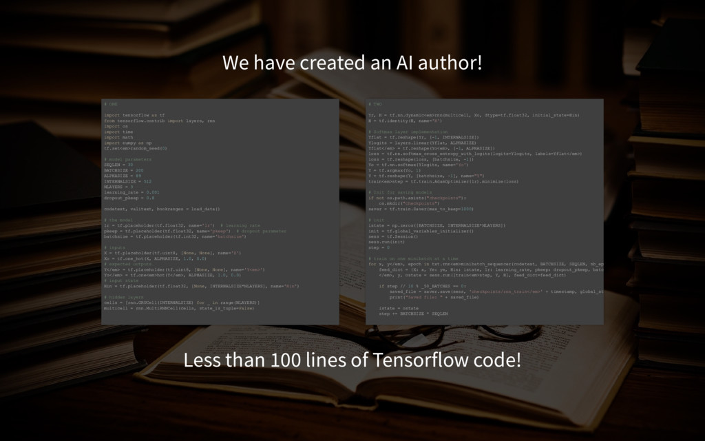
of Tensorflow code! # ONE import tensorflow as tf from tensorflow.contrib import layers, rnn import os import time import math import numpy as np tf.set<em>random_seed(0) # model parameters SEQLEN = 30 BATCHSIZE = 200 ALPHASIZE = 89 INTERNALSIZE = 512 NLAYERS = 3 learning_rate = 0.001 dropout_pkeep = 0.8 codetext, valitext, bookranges = load_data() # the model lr = tf.placeholder(tf.float32, name='lr') # learning rate pkeep = tf.placeholder(tf.float32, name='pkeep') # dropout parameter batchsize = tf.placeholder(tf.int32, name='batchsize') # inputs X = tf.placeholder(tf.uint8, [None, None], name='X') Xo = tf.one_hot(X, ALPHASIZE, 1.0, 0.0) # expected outputs Y</em> = tf.placeholder(tf.uint8, [None, None], name='Y<em>') Yo</em> = tf.one<em>hot(Y</em>, ALPHASIZE, 1.0, 0.0) # input state Hin = tf.placeholder(tf.float32, [None, INTERNALSIZE*NLAYERS], name='Hin') # hidden layers cells = [rnn.GRUCell(INTERNALSIZE) for _ in range(NLAYERS)] multicell = rnn.MultiRNNCell(cells, state_is_tuple=False) # TWO Yr, H = tf.nn.dynamic<em>rnn(multicell, Xo, dtype=tf.float32, initial_state=Hin) H = tf.identity(H, name='H') # Softmax layer implementation Yflat = tf.reshape(Yr, [1, INTERNALSIZE]) Ylogits = layers.linear(Yflat, ALPHASIZE) Yflat</em> = tf.reshape(Yo<em>, [1, ALPHASIZE]) loss = tf.nn.softmax_cross_entropy_with_logits(logits=Ylogits, labels=Yflat</em>) loss = tf.reshape(loss, [batchsize, 1]) Yo = tf.nn.softmax(Ylogits, name='Yo') Y = tf.argmax(Yo, 1) Y = tf.reshape(Y, [batchsize, 1], name="Y") train<em>step = tf.train.AdamOptimizer(lr).minimize(loss) # Init for saving models if not os.path.exists("checkpoints"): os.mkdir("checkpoints") saver = tf.train.Saver(max_to_keep=1000) # init istate = np.zeros([BATCHSIZE, INTERNALSIZE*NLAYERS]) init = tf.global_variables_initializer() sess = tf.Session() sess.run(init) step = 0 # train on one minibatch at a time for x, y</em>, epoch in txt.rnn<em>minibatch_sequencer(codetext, BATCHSIZE, SEQLEN, nb_ep feed_dict = {X: x, Ye: ye, Hin: istate, lr: learning_rate, pkeep: dropout_pkeep, batc </em>, y, ostate = sess.run([train<em>step, Y, H], feed_dict=feed_dict) if step // 10 % _50_BATCHES == 0: saved_file = saver.save(sess, 'checkpoints/rnn_train</em>' + timestamp, global_st print("Saved file: " + saved_file) istate = ostate step += BATCHSIZE * SEQLEN
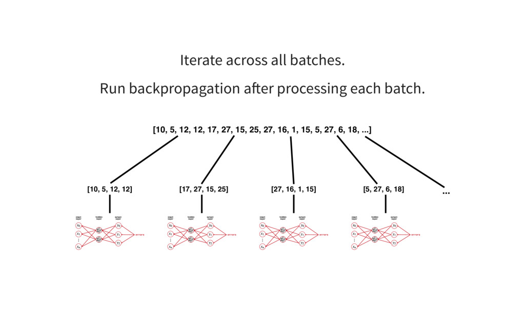
![['h','e','l','l','o',' ', 'm','y',' ','n','a','m','e',' ','i','s', ...] [10, 5, 12, 12,](https://files.speakerdeck.com/presentations/c3e63fb3ec2f4e1cb18b0ff676cd85dc/slide_6.jpg)
![ACTIVATION FUNCTION SIGMOID FUNCTION Squashes perceptron output into range [0,1]](https://files.speakerdeck.com/presentations/c3e63fb3ec2f4e1cb18b0ff676cd85dc/slide_28.jpg)
![['h','e','l','l','o',' ', 'm','y',' ','n','a','m','e',' ','i','s', ...] [10, 5, 12, 12,](https://files.speakerdeck.com/presentations/c3e63fb3ec2f4e1cb18b0ff676cd85dc/slide_87.jpg)
![GET IN TOUCH don@donso .io @donald_whyte https://github.com/DonaldWhyte [email protected] @AxSaucedo https://github.com/axsauze](https://files.speakerdeck.com/presentations/c3e63fb3ec2f4e1cb18b0ff676cd85dc/slide_137.jpg)