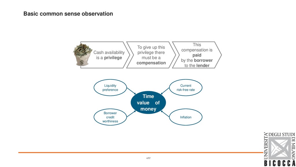
give up this privilege there must be a compensation This compensation is paid by the borrower to the lender Inflation Time value of money Current risk-free rate Liquidity preference Borrower credit worthiness 4/97
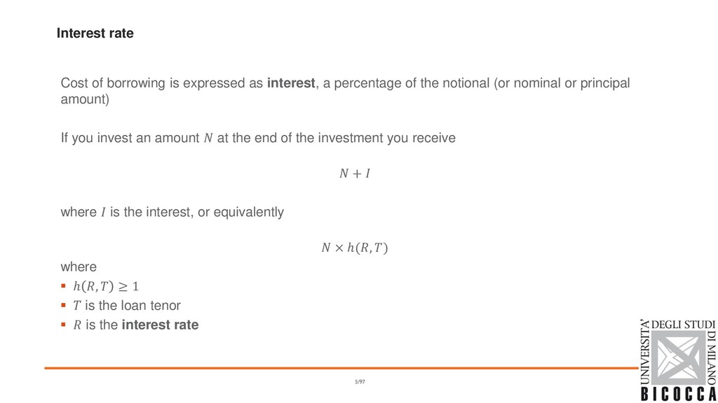
percentage of the notional (or nominal or principal amount) If you invest an amount at the end of the investment you receive + where is the interest, or equivalently × ℎ(, ) where ▪ ℎ , ≥ 1 ▪ is the loan tenor ▪ is the interest rate 5/97
value (in T) of one unit of currency paid today ▪ How many units of currency received in are equivalent to 1 unit of currency received today? , Discount factor ▪ The present value (today) of one unit of currency paid at time T ▪ How many units of currency received today are equivalent to 1 unit of currency received in ? toda y T 1 ℎ(, ) toda y T 1 1 ℎ(, ) 6
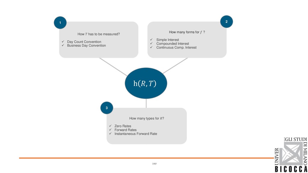
Day Count Convention ✓ Business Day Convention How many types for ? ✓ Zero Rates ✓ Forward Rates ✓ Instantaneous Forward Rate How many forms for ? ✓ Simple Interest ✓ Compounded Interest ✓ Continuous Comp. Interest h , 1 2 3 7/97
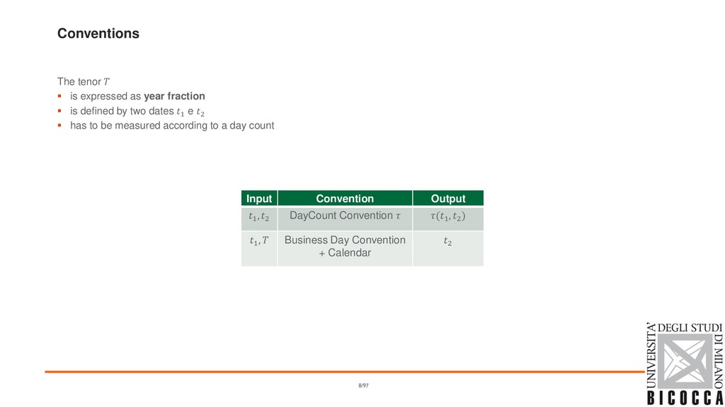
is defined by two dates 1 e 2 ▪ has to be measured according to a day count 8/97 Input Convention Output 1 , 2 DayCount Convention (1 , 2 ) 1 , Business Day Convention + Calendar 2
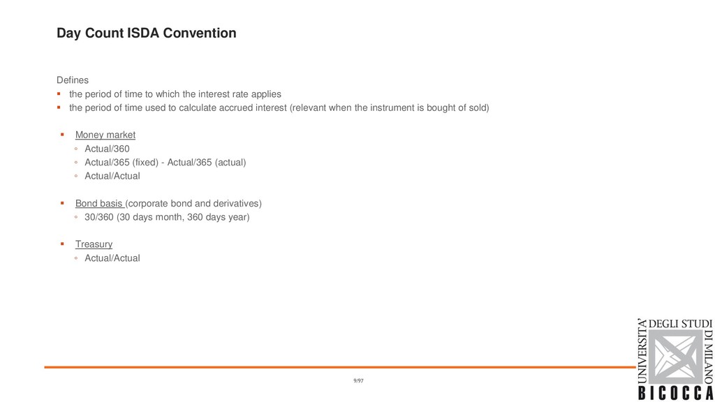
to which the interest rate applies ▪ the period of time used to calculate accrued interest (relevant when the instrument is bought of sold) ▪ Money market ◦ Actual/360 ◦ Actual/365 (fixed) - Actual/365 (actual) ◦ Actual/Actual ▪ Bond basis (corporate bond and derivatives) ◦ 30/360 (30 days month, 360 days year) ▪ Treasury ◦ Actual/Actual 9/97
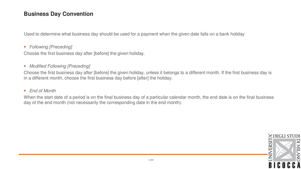
be used for a payment when the given date falls on a bank holiday ▪ Following [Preceding] Choose the first business day after [before] the given holiday. ▪ Modified Following [Preceding] Choose the first business day after [before] the given holiday, unless it belongs to a different month. If the first business day is in a different month, choose the first business day before [after] the holiday. ▪ End of Month When the start date of a period is on the final business day of a particular calendar month, the end date is on the final business day of the end month (not necessarily the corresponding date in the end month). 11/97
◦ 4% is earned between coupon payment dates. Accruals on an Actual basis. When coupons are paid on March 1 and Sept 1, how much interest is earned between March 1 and April 1? ▪ Bond 8% 30/360 ◦ Assumes 30 days per month and 360 days per year. When coupons are paid on March 1 and Sept 1, how much interest is earned between March 1 and April 1? ▪ T-Bill 8% Actual/360 ◦ 8% is earned in 360 days. Accrual calculated by dividing the actual number of days in the period by 360. How much interest is earned between March 1 and April 1? 13/97
) years at rate an amount grows to × 1 + Usually the interest is payed ▪ At the end of the period for tenor less than 1Y ▪ Annualy for longer tenors Capitalization factor ℎ , = 1 + Discount factor 1 ℎ , = 1 + − Compounded Interest 14/97
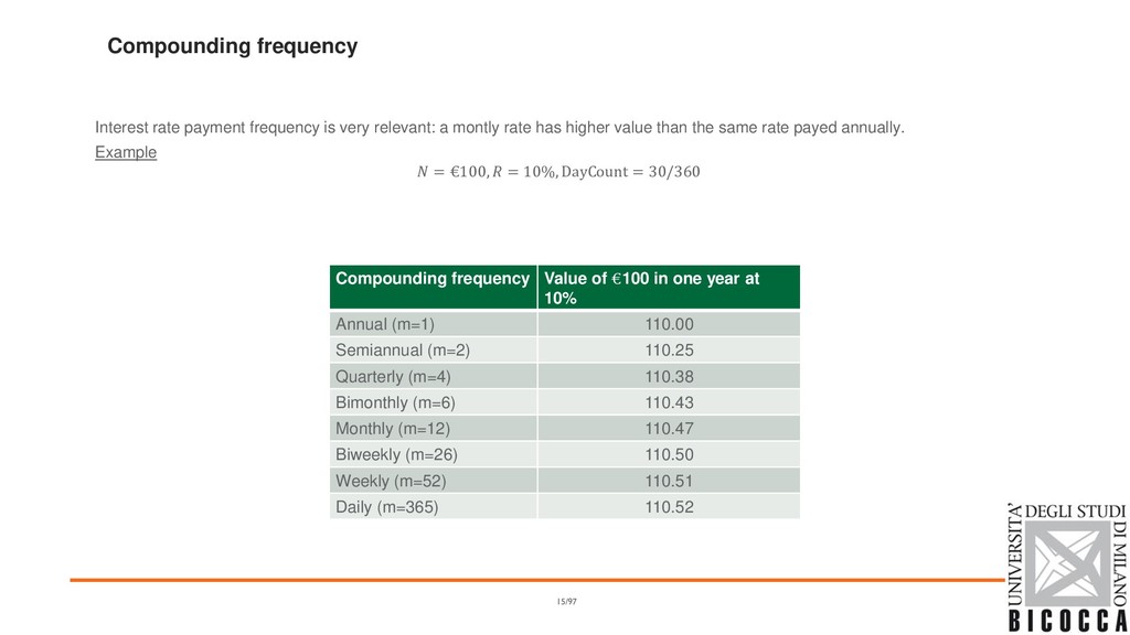
montly rate has higher value than the same rate payed annually. Example = €100, = 10%, DayCount = 30/360 Compounding frequency Value of €100 in one year at 10% Annual (m=1) 110.00 Semiannual (m=2) 110.25 Quarterly (m=4) 110.38 Bimonthly (m=6) 110.43 Monthly (m=12) 110.47 Biweekly (m=26) 110.50 Weekly (m=52) 110.51 Daily (m=365) 110.52 15/97
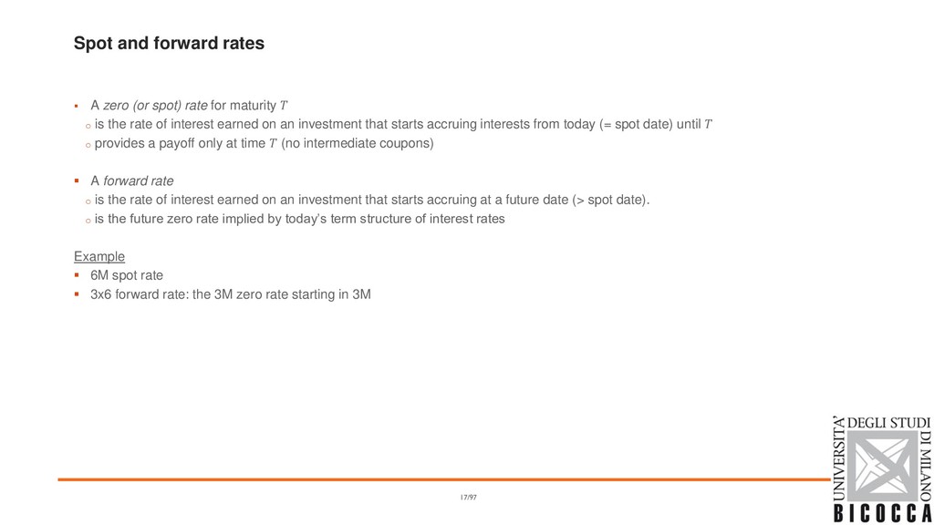
for maturity o is the rate of interest earned on an investment that starts accruing interests from today (= spot date) until o provides a payoff only at time (no intermediate coupons) ▪ A forward rate o is the rate of interest earned on an investment that starts accruing at a future date (> spot date). o is the future zero rate implied by today’s term structure of interest rates Example ▪ 6M spot rate ▪ 3x6 forward rate: the 3M zero rate starting in 3M 17/97
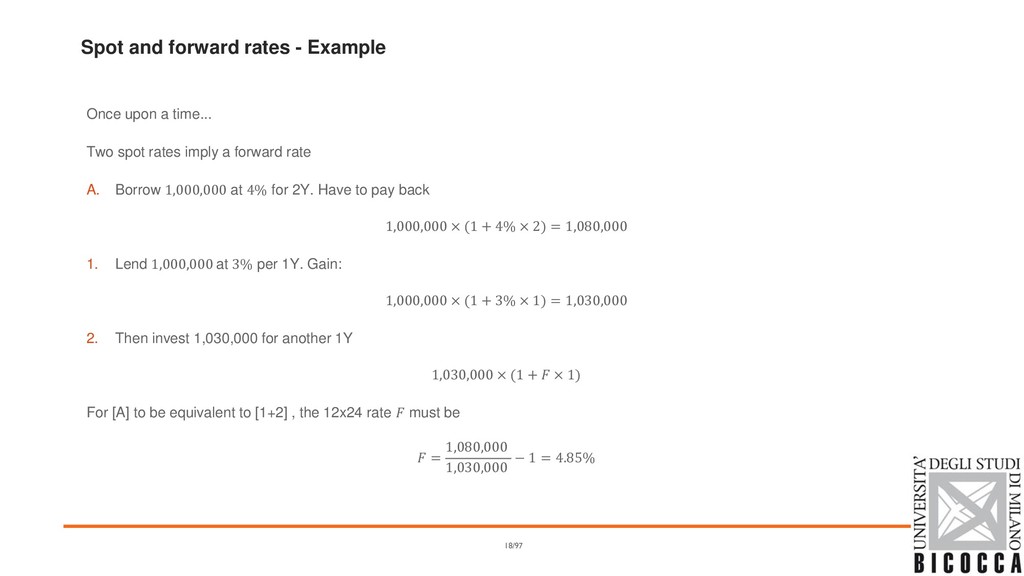
Two spot rates imply a forward rate A. Borrow 1,000,000 at 4% for 2Y. Have to pay back 1,000,000 × (1 + 4% × 2) = 1,080,000 1. Lend 1,000,000 at 3% per 1Y. Gain: 1,000,000 × (1 + 3% × 1) = 1,030,000 2. Then invest 1,030,000 for another 1Y 1,030,000 × (1 + × 1) For [A] to be equivalent to [1+2] , the 12x24 rate must be = 1,080,000 1,030,000 − 1 = 4.85% 18/97
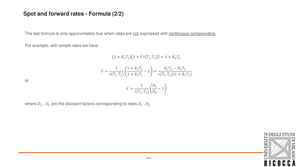
zero rates for time periods 1 and 2 are 1 and 2 with both rates continuously compounded The forward rate for the period between times 1 and 2 satisfies 1(0,1)(1,2) = 2(0,2) So we have = 2 (0, 2 ) − 1 (0, 1 ) (1 , 2 ) 19/97
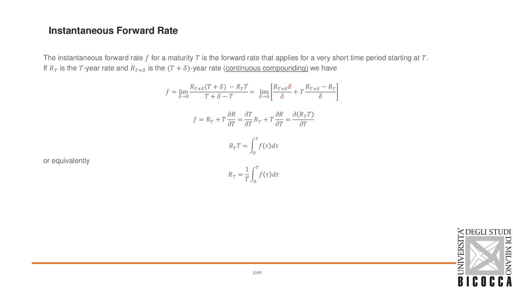
rate that applies for a very short time period starting at . If is the -year rate and + is the ( + )-year rate (continuous compounding) we have = lim →0 + ( + ) − + − = lim →0 + + + − = + = + = = න 0 or equivalently = 1 න 0 Instantaneous Forward Rate 23/97
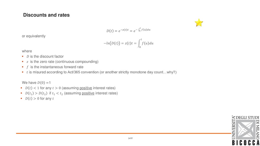
= න 0 where ▪ is the discount factor ▪ is the zero rate (continuous compounding) ▪ is the instantaneous forward rate ▪ is misured according to Act/365 convention (or another strictly monotone day count…why?) We have 0 =1 ▪ < 1 for any > 0 (assuming positive interest rates) ▪ 1 > 2 if 1 < 2 (assuming positive interest rates) ▪ > 0 for any Discounts and rates 24/97
by a government in its own currency. ▪ LIBOR rate: the rate of interest at which a bank is prepared to deposit money with another bank (the second bank must typically have a AA rating). ▪ LIBID rate: the rate which a AA bank is prepared to pay on deposits from another bank. ▪ Eurodollar futures and swaps are used to extend the LIBOR yield curve beyond one year. 25/97
at which a bank is prepared to lend to another bank for just one day. ▪ Repo rates: Repurchase agreement is an agreement where a financial institution that owns securities agrees to sell them today for X and buy them back in the future for a slightly higher price Y ◦ The financial institution obtains a loan ◦ The rate of interest is calculated from the difference between X and Y and is known as the repo rate 26/97
start at reference date 0 (today or spot), span the length corresponding to their maturity and pay the (annual, simply compounded) interest accrued over the period with a given rate fixed at 0 ▪ Maturities o O/N (overnight), T/N (tomorrow-next), S/N (spot-next) o 1W or SW (spot-week) o 1M, 2M, 3M, 6M, 9M, 12M ▪ Deposit Rates are o illiquid o not collateralized (to be explained later) o not representative of Libor/Euribor fixings (which are the underlying of collateralized interest rate derivatives) 29/97
is an OTC agreement that a certain rate will apply to a certain principal during a certain future time period ▪ FRAs pay the difference between a given strike and the underlying Euribor fixing ▪ 4x7 stands for 3M Euribor fixing in 4 months time ▪ The market quotes FRA strips with different fixing dates and Libor/Euribor tenors 33/97
an agreement where interest at a predetermined rate is exchanged for interest at the market rate A FRA can be valued by assuming that the forward LIBOR interest rate is certain to be realized This means that the value of a FRA is the present value of the difference between the interest that would be paid at rate and the interest that would be paid at rate 34/97
applies lasts from 1 to 2, we assume that and are expressed with a compounding frequency corresponding to the length of the period between 1 and 2 With an interest rate of , the interest cash flow at time 2 is (1 , 2 ) With an interest rate of , the interest cash flow at time 2 is (1 , 2 ) 35/97
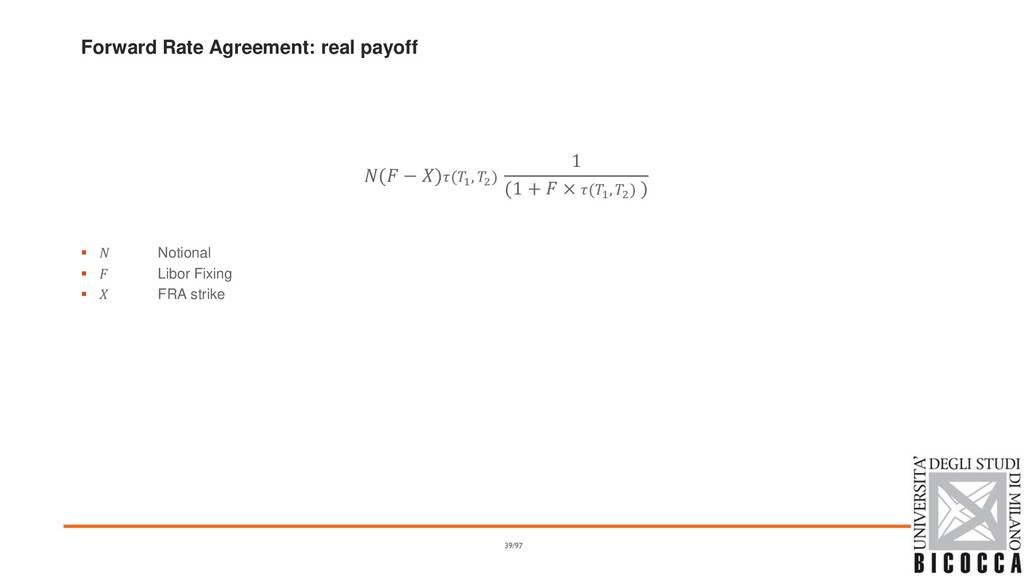
on a principal of the value of the FRA is the present value of ( − )(1 , 2 ) received at time 2 ▪ When the rate will be paid on a principal of the value of the FRA is the present value of ( − )(1 , 2 ) received at time 2 36/97
ensures that a company will receive 4% (s.a.) on $100 million for six months starting in 1 year ▪ Forward LIBOR current estimation for the period is 5% (s.a.) ▪ The 1.5 year rate is 4.5% with continuous compounding The value of the FRA (in $ millions) is 100 × 0.04 − 0.05 × 0.5 × −0.045×1.5 = −0.467 37/97
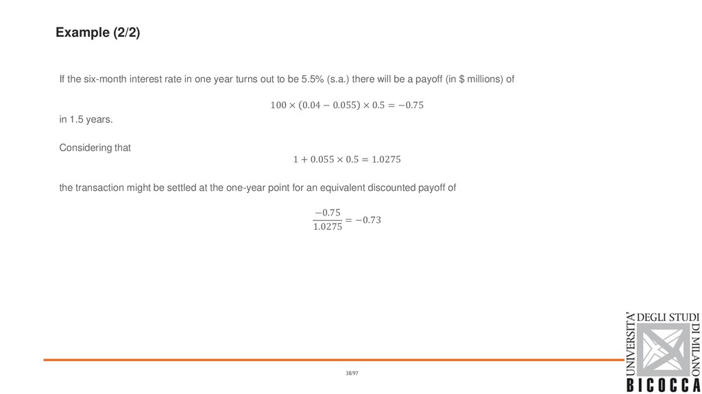
turns out to be 5.5% (s.a.) there will be a payoff (in $ millions) of 100 × 0.04 − 0.055 × 0.5 = −0.75 in 1.5 years. Considering that 1 + 0.055 × 0.5 = 1.0275 the transaction might be settled at the one-year point for an equivalent discounted payoff of −0.75 1.0275 = −0.73 38/97
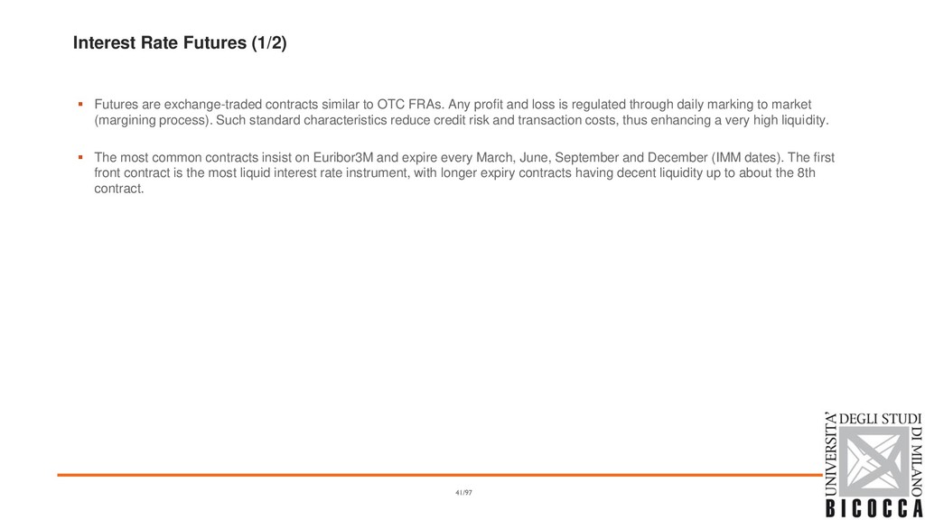
to OTC FRAs. Any profit and loss is regulated through daily marking to market (margining process). Such standard characteristics reduce credit risk and transaction costs, thus enhancing a very high liquidity. ▪ The most common contracts insist on Euribor3M and expire every March, June, September and December (IMM dates). The first front contract is the most liquid interest rate instrument, with longer expiry contracts having decent liquidity up to about the 8th contract. 41/97
called serial futures, expiring in the upcoming months not covered by the quarterly IMM futures. The first serial contract is quite liquid, especially when it expires before the front contract. ▪ Futures are quoted in terms of prices instead of rates. The relation is = 100 − To mimic the bond behavior of increasing prices for decreasing rates (see later) 42/97
a bank outside the United States. ▪ Eurodollar Futures are futures on the 3-month Eurodollar deposit rate (same as 3-month LIBOR rate) ▪ It is margined every day ▪ It is settled in cash ▪ When it expires (on the third Wednesday of the delivery month) the final settlement price is 100 minus the actual three month Eurodollar deposit rate 43/97
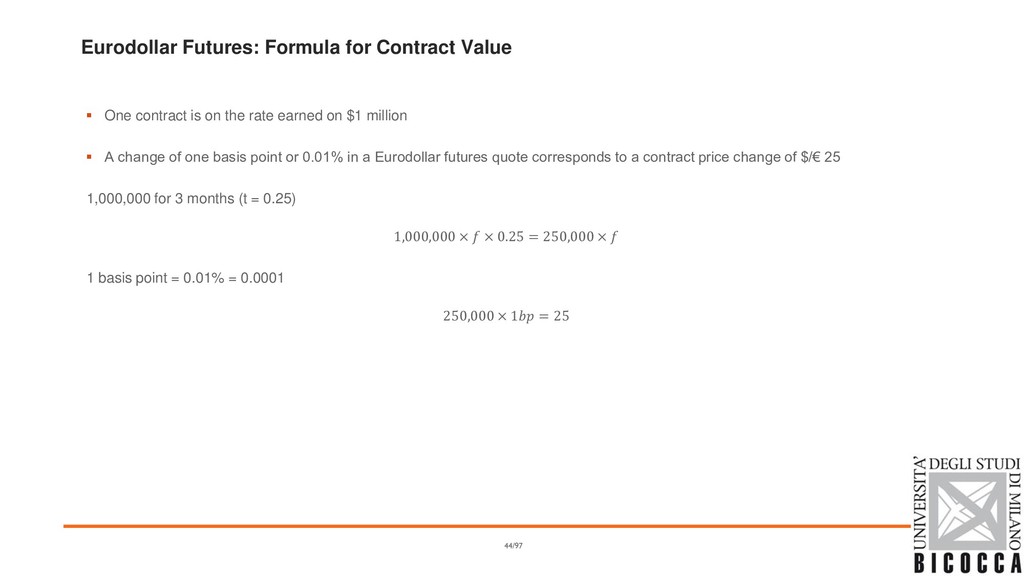
on the rate earned on $1 million ▪ A change of one basis point or 0.01% in a Eurodollar futures quote corresponds to a contract price change of $/€ 25 1,000,000 for 3 months (t = 0.25) 1,000,000 × × 0.25 = 250,000 × 1 basis point = 0.01% = 0.0001 250,000 × 1 = 25 44/97
in) a contract on Nov 1 ▪ The contract expires on Dec 21 ▪ The prices are as shown in table ▪ How much do you gain or lose o on the first day o on the second day o over the whole time until expiration Date Quote Nov 1 97.12 Nov 2 97.23 Nov 3 96.98 ……. …… Dec 21 97.42 45/97
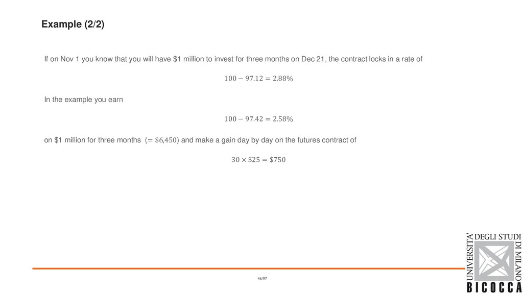
will have $1 million to invest for three months on Dec 21, the contract locks in a rate of 100 − 97.12 = 2.88% In the example you earn 100 − 97.42 = 2.58% on $1 million for three months (= $6,450) and make a gain day by day on the futures contract of 30 × $25 = $750 46/97
marking to market an investor short on a futures contract ▪ when the futures price increases (rate decreases) has a loss that can be funded at lower rate ▪ when the futures price decreases (rate increases) has a profit that can be invested at higher rate Short futures, long FRA generates free money: there is a convexity to be compensated with lower futures price (higher rate) = + 47/97
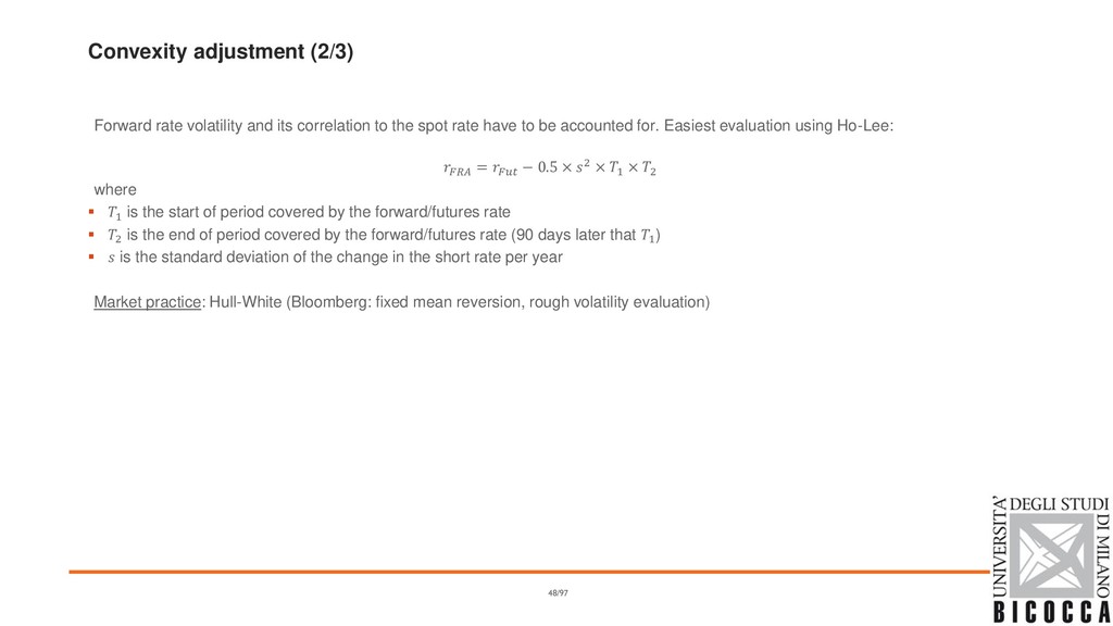
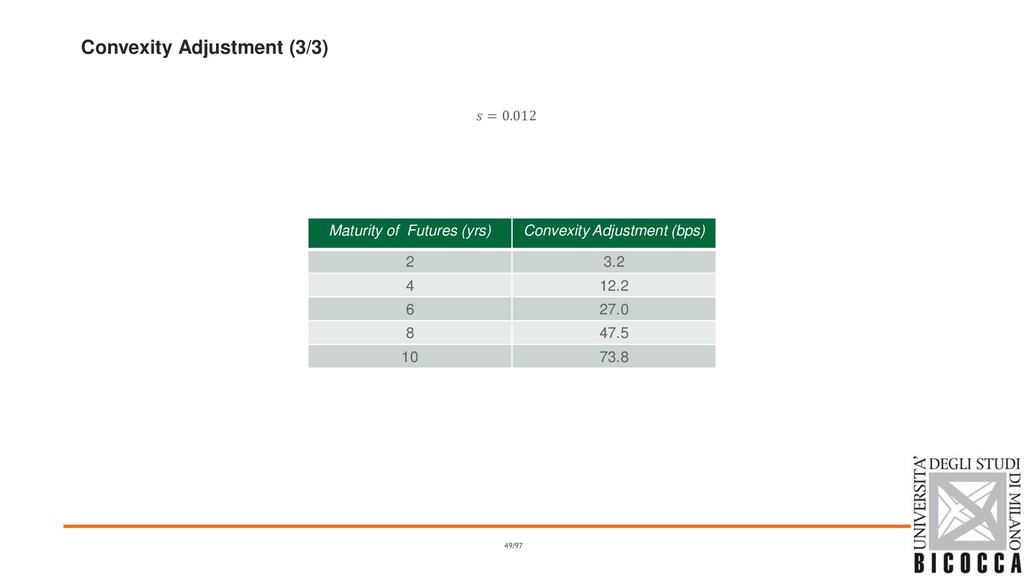
the spot rate have to be accounted for. Easiest evaluation using Ho-Lee: = − 0.5 × 2 × 1 × 2 where ▪ 1 is the start of period covered by the forward/futures rate ▪ 2 is the end of period covered by the forward/futures rate (90 days later that 1) ▪ is the standard deviation of the change in the short rate per year Market practice: Hull-White (Bloomberg: fixed mean reversion, rough volatility evaluation) 48/97
the LIBOR zero curve out to one year ▪ Eurodollar futures can be used to determine forward rates and the forward rates can then be used to bootstrap the zero curve 50/97
Interest ▪ The quoted price is called clean price because it is free from the deterministic price change effect of accruing interest ▪ The cash price is also called dirty price 52/97
makes the present value of the cash flows on the bond equal to the market price of the bond Suppose that the market price of the bond in our example equals its theoretical price of 98.39. The bond yield (continuously compounded) is given by solving 3−×0.5 + 3−×1.0 + 3−×1.5 + 103−×2.0 = 98.39 to get = 0.0676 = 6.76% 53/97
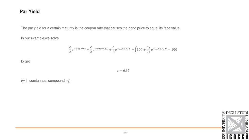
the coupon rate that causes the bond price to equal its face value. In our example we solve 2 −0.05×0.5 + 2 −0.058×1.0 + 2 −0.064×1.5 + 100 + 2 −0.068×2.0 = 100 to get = 6.87 (with semiannual compounding) 54/97
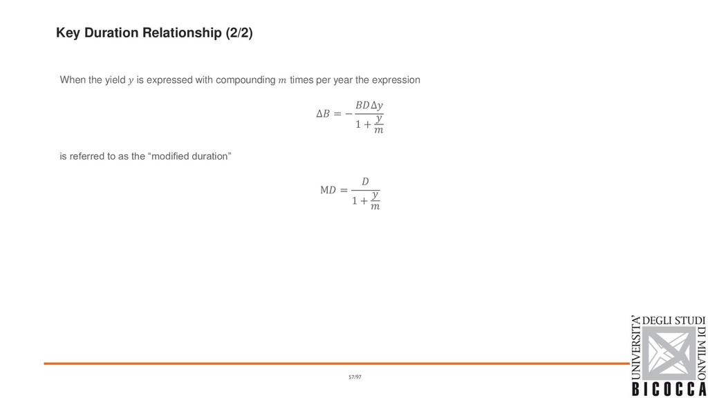
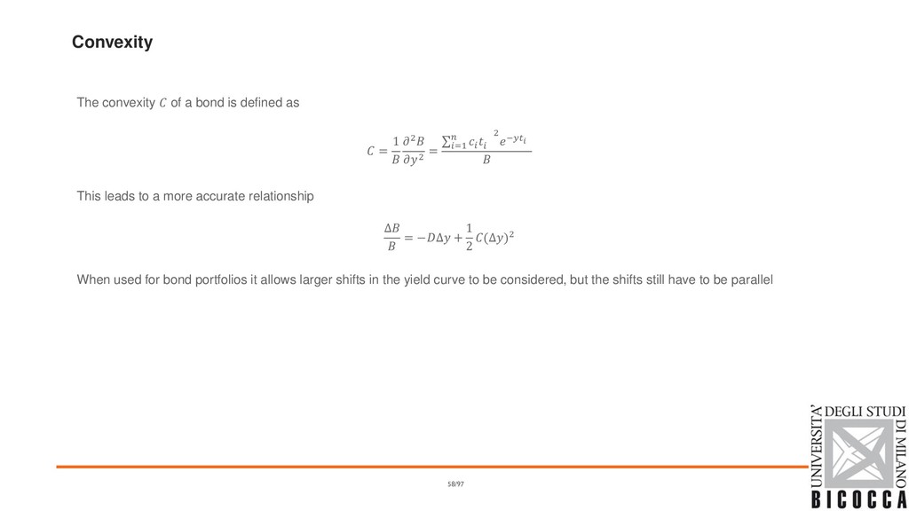
1 2 2 = σ =1 2 − This leads to a more accurate relationship ∆ = −∆ + 1 2 (∆)2 When used for bond portfolios it allows larger shifts in the yield curve to be considered, but the shifts still have to be parallel 58/97
the weighted average duration of the bonds in the portfolio with weights proportional to prices ▪ The key duration relationship for a bond portfolio describes the effect of small parallel shifts in the yield curve ▪ What exposures remain if duration of a portfolio of assets equals the duration of a portfolio of liabilities? 59/97
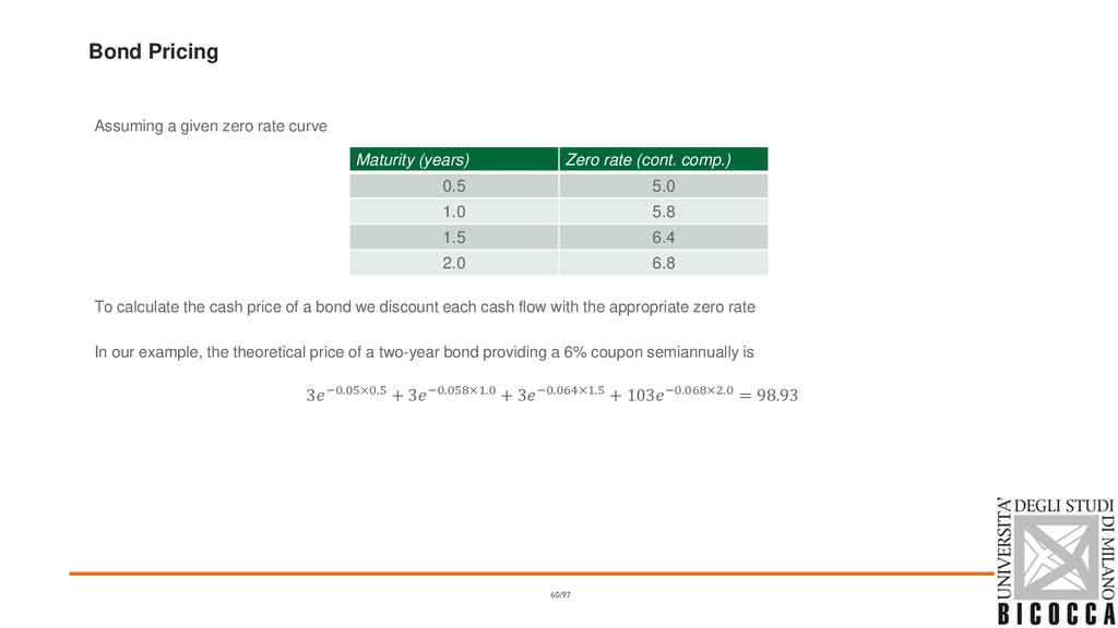
the cash price of a bond we discount each cash flow with the appropriate zero rate In our example, the theoretical price of a two-year bond providing a 6% coupon semiannually is 3−0.05×0.5 + 3−0.058×1.0 + 3−0.064×1.5 + 103−0.068×2.0 = 98.93 Maturity (years) Zero rate (cont. comp.) 0.5 5.0 1.0 5.8 1.5 6.4 2.0 6.8 60/97
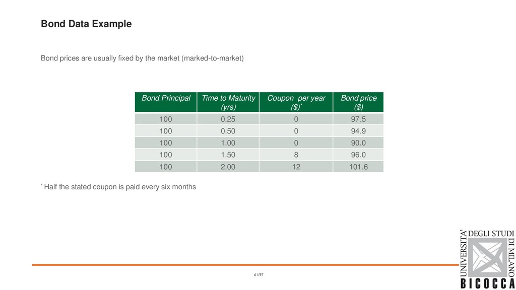
market (marked-to-market) * Half the stated coupon is paid every six months 61/97 Bond Principal Time to Maturity (yrs) Coupon per year ($)* Bond price ($) 100 0.25 0 97.5 100 0.50 0 94.9 100 1.00 0 90.0 100 1.50 8 96.0 100 2.00 12 101.6
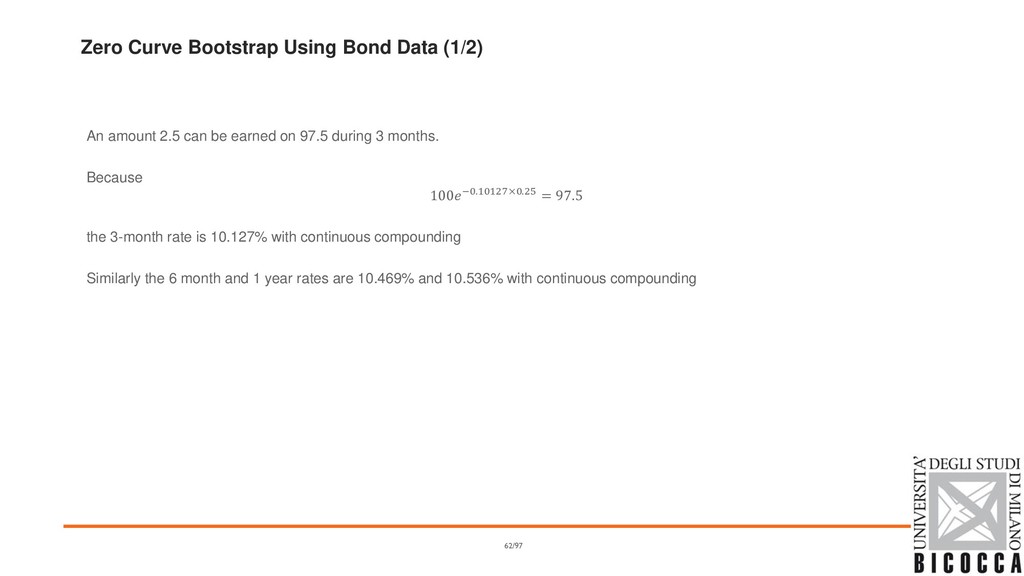
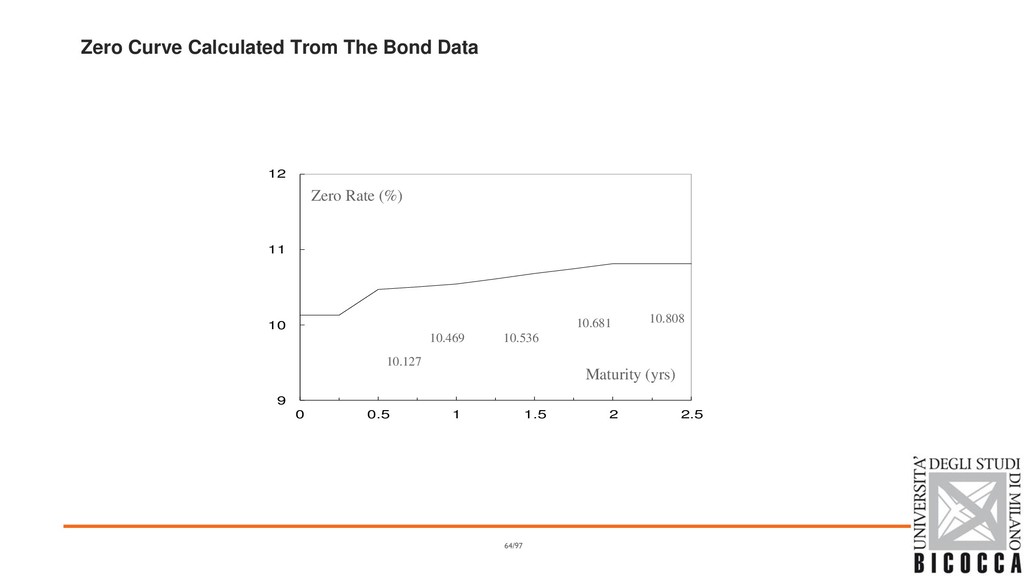
can be earned on 97.5 during 3 months. Because 100−0.10127×0.25 = 97.5 the 3-month rate is 10.127% with continuous compounding Similarly the 6 month and 1 year rates are 10.469% and 10.536% with continuous compounding 62/97
exchange cash flows at specified future times according to certain specified rules ▪ Vanilla swaps are OTC contracts in which two counterparties agree to exchange fixed against floating rate cash flows ▪ The EUR market quotes standard plain vanilla swaps starting at spot date with annual fixed leg versus floating leg indexed to 6M (or 3M) Euribor rate ▪ Swaps can be regarded as weighted portfolios of 6M (or 3M) FRA 66/97
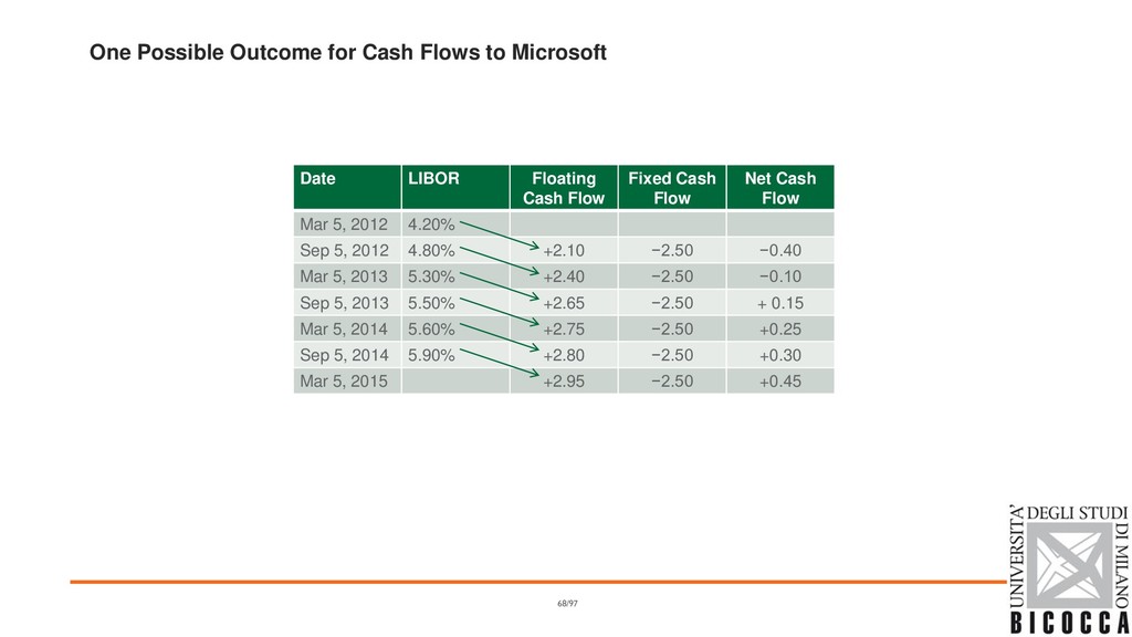
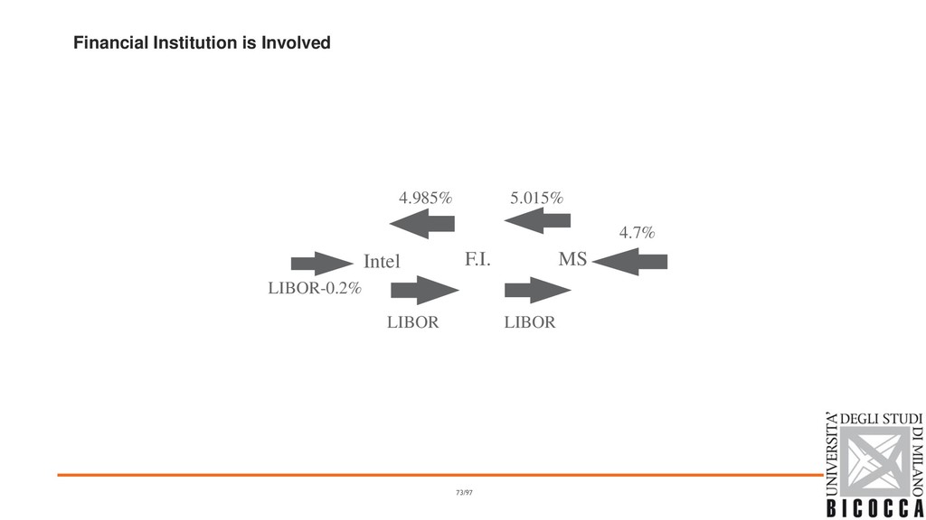
agreement by Microsoft to ▪ receive 6-month LIBOR ▪ pay a fixed rate of 5% per annum every 6 months for 3 years on a notional principal of $100 million Next slide illustrates cash flows that could occur (day count conventions are not considered) 67/97
from ▪ fixed rate to floating rate ▪ floating rate to fixed rate Converting an investment from ▪ fixed rate to floating rate ▪ floating rate to fixed rate 69/97
The International Swaps and Derivatives Association (ISDA) has developed Master Agreements that can be used to cover all agreements between two counterparties ▪ Governments now require central clearing to be used for most standardized derivatives 75/97
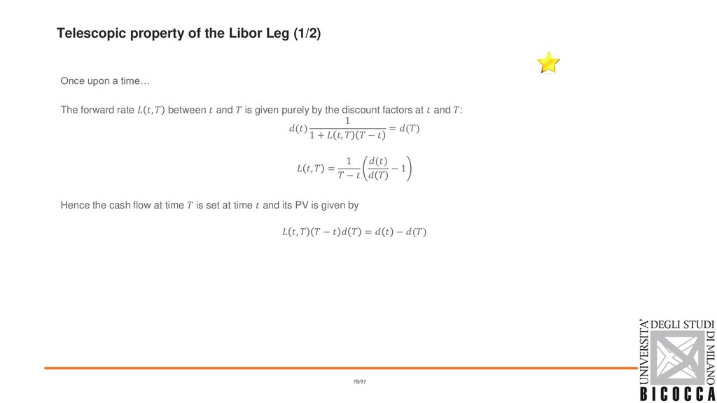
time… The forward rate , between and is given purely by the discount factors at and : () 1 1 + , − = () , = 1 − () − 1 Hence the cash flow at time is set at time and its PV is given by , − = − () 78/97
time… If you sum up all the cash flows then the intermediate discount factors all drop out and the PV of the floating leg is = =0 , +1 +1 − +1 = = =0 − +1 = 0 − 79/97
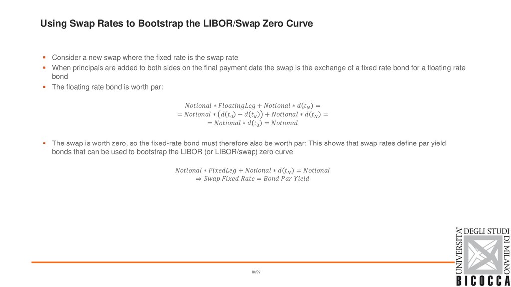
Consider a new swap where the fixed rate is the swap rate ▪ When principals are added to both sides on the final payment date the swap is the exchange of a fixed rate bond for a floating rate bond ▪ The floating rate bond is worth par: ∗ + ∗ = = ∗ 0 − + ∗ = = ∗ 0 = ▪ The swap is worth zero, so the fixed-rate bond must therefore also be worth par: This shows that swap rates define par yield bonds that can be used to bootstrap the LIBOR (or LIBOR/swap) zero curve ∗ + ∗ = ֜ = 80/97
zero rates are 4%, 4.5% and 4.8% with continuous compounding. Two-year swap rate is 5% (2.5% in 6 months) 2.5−0.04×0.5 + 2.5−0.045×1.0 + 2.5−0.048×1.5 + 102.5−×2.0 = 100 The 2-year zero rate is = 4.953% 81/97
Swaps are worth close to zero ▪ At later times they can be valued as the difference between the value of a fixed-rate bond and the value of a floating-rate bond ▪ Alternatively, they can be valued as a portfolio of Forward Rate Agreements (FRAs) 82/97
for the overnight rate ▪ The overnight rate is compounded and paid at maturity ▪ On both legs there is o a single payment for maturity up to 1Y o yearly payments with short stub for longer maturities 83/97
is exchanged for the geometric average of the overnight rates ▪ Should OIS rate equal the LIBOR rate? A bank can o Borrow $100 million in the overnight market, rolling forward for 3 months o Enter into an OIS swap to convert this to the 3-month OIS rate o Lend the funds to another bank at LIBOR for 3 months ...but it bears the credit risk of another bank in this arrangement ▪ The OIS rate is now regarded as a better proxy for the short-term risk-free rate than LIBOR ▪ The excess of LIBOR over the OIS rate is the LIBOR-OIS spread 84/97
a convenient way of packaging forward contracts ▪ Although the swap contract is usually worth close to zero at the outset, each of the underlying forward contracts are not worth zero 85/97
company initially. At a future time its value is liable to be either positive or negative ▪ The company has credit risk exposure only when its value is positive ▪ Some swaps are more likely to lead to credit risk exposure than others o What is the situation if early forward rates have a positive value? o What is the situation when early forward rates have a negative value? 86/97
usually floating vs floating swaps with different tenors on the two legs ▪ The EUR market quotes standard plain vanilla basis swaps as portfolios of two regular fixed-floating swaps with the floating legs paying different Euribor indexes. The quotation convention is to provide the difference (in basis points) between the fixed rates of the two regular swaps. ▪ Basis is positive and decreasing with maturity, reflecting the preference of market players for receiving payments with higher frequency (e.g. 3M instead of 6M, 6M instead of 12M, etc.) and shorter maturities ▪ Basis swaps allow to imply levels for non-quoted swaps on Euribor 1M and 12M from the quoted swap rates on Euribor 6M 88/97
a basket of financial instruments and its variations over time: its value is the weighted average (according to a certain method) of the prices of instruments included in the portfolio ▪ An Interest Rate Index is based on the interest rate of a financial instrument or basket of financial instruments an it serves as a benchmark used to calculate the interest rate charged on financial products 90/97
interbank lending between one day and one year ▪ They are usually computed as the trimmed average between rates contributed by participating banks ▪ The rates are banks' estimates but usually do not refer to actual transactions ▪ The most common usage of those indexes in interest rate derivatives is in swaps and caps/floors 91/97
interbank term deposits are offered by one prime bank to another prime bank within the EMU zone. ▪ ICE LIBOR (London Inter Bank Offered Rate): benchmark rate produced for five currencies (CHF, EUR, GBP, JPY, USD) with seven maturities quoted for each (ranging from overnight to 12 months) producing 35 rates each business day. It provides an indication of the average rate at which a LIBOR contributor bank can obtain unsecured funding in the London interbank market for a given period, in a given currency. 92/97
swap rates ▪ They are usually computed as trimmed average between mid-market rates contributed by participating banks ▪ The most common usage of these indexes is in Constant Maturity Swaps (CMS) Example ▪ ISDAFIX: a benchmark for annual swap rates for interest rate swap transactions; it represents average mid-market rates for vanilla fixed- for-floating interest rate swaps in three major currencies (USD, EUR, GBP) at selected maturities on a daily basis. 93/97
interbank lending on a one day horizon ▪ Most indexes are for overnight loans and some for tomorrow/next loans ▪ The rates are computed as a weighted average of actual transactions ▪ The most common usage of those indexes in interest rate derivatives is in overnight indexed swaps 94/97
Average): the effective overnight reference rate for the Euro, computed as a weighted average of all overnight unsecured lending transactions in the interbank market, undertaken in the European Union and European Free Trade Association (EFTA) countries. ▪ Sonia (Sterling Over Night Index Average): the weighted average rate to four decimal places of all unsecured sterling overnight cash transactions brokered in London by contributing WMBA member firms between 00:00 hrs and 16:15 hrs UK time with all counterparties in a minimum deal size of £25 million. 95/97