Rate Curves Calibration

Discounting and Forwarding Curves Models and Implementation Rate Curves Calibration
Ferdinando M. Ametrano https://www.ametrano.net/about/

Rate curve term structure: more an art than a science
▪ Pricing complex Interest Rate Derivatives requires modeling the future dynamics of the rate curve term structure ▪ Any modeling approach will fail to produce good/reasonable prices if the current term structure is not correct ▪ Most of the literature assumes the existence of the current rate curve as given and its construction is often neglected or even obscured ▪ Financial institutions, software houses and practitioners have developed their own proprietary methodologies in order to extract the rate curve term structure from quoted prices of a finite number of liquid market instruments 2/91

Outline 1. Rate curve parameterization: discretization and interpolation scheme 2.
Rate curve bootstrapping 3. Turn of Year 4. The standard rate curve 5. What has changed since summer 2007 6. Multiple forwarding rate curves 7. Discounting rate curve 8. Bibliography 3/91

Interest Rate Curves Calibration - Basics 1. Rate curve parameterization:
discretization and interpolation scheme

Rate curve parameterization = − = − ׬ 0 or
equivalently − = = න 0 Discrete time-grid of ▪ discount factors ▪ continuous (sometime compounded) zero rates ▪ instantaneous continuous forward rates ▪ 0 = 1 (only discount factors are well defined at = 0) ▪ > 0 for any ▪ < 1 for any > 0 (assuming positive interest rates) ▪ 1 > 2 if 1 < 2 (assuming positive interest rates) 5/91

Interpolation Whatever parameterization has been chosen, an interpolation for off-grid
dates/times is needed ▪ Discount factors have exponential decay so it makes sense to interpolate on log-discounts ▪ A (poor) common choice is to interpolate (linearly) on zero rates: linear interpolation is easy and local (it only depends on the 2 surrounding points) ▪ The smoothness of a rate curve is to be measured on the smoothness of its (simple) forward rates: so it would make sense to use a smooth interpolation on (instantaneous continuous) forward rates 6/91

Local scheme vs global scheme LOCAL SCHEME GLOBAL SCHEME GLOBAL
SCHEME 7/42

Linear interpolation on log-discounts It generates piecewise flat forward rates
Euribor 6M Curve – March 10, 2015 8/91

Linear interpolation on zero rates It generates sawtooth forward rates

Linear interpolation on forward rates It generates non-smooth forward rates

Monotonic cubic interpolation on log-discounts It generates smooth forward rates

Smoothness beyond linear: cubic interpolations A cubic interpolation is fully
defined when the function values at points are supplemented with function derivative values ′ Different type of first derivative approximations are available: ▪ Local schemes (Fourth-order, Parabolic, Fritsch-Butland, Akima, Kruger, etc) use only values near to calculate each ′ ▪ Non-local schemes (spline with different boundary conditions) use all values and obtain ′ by solving a linear system of equations Local schemes produce 1 interpolants, while the spline schemes generate 2 interpolants 12/91

Cubic interpolation problems Simple cubic interpolations suffer of well-documented problems
such as ▪ spurious inflection points ▪ excessive convexity ▪ lack of locality Wide oscillation can generate negative forward rates o Andersen has addressed these issues through the use of shape-preserving splines from the class of generalized tension splines o Hagan and West have developed a new scheme based on positive preserving forward interpolation 13/91

Monotonic cubic interpolation: Hyman filter Hyman monotonic filter is the
simpler, more general, most effective approach to avoid spurious excessive oscillation It can be applied to all schemes to ensure that in the regions of local monotonicity of the input (three successive increasing or decreasing values) the interpolating cubic remains monotonic. If the interpolating cubic is already monotonic, the Hyman filter leaves it unchanged preserving all its original features. In the case of 2 interpolants the Hyman filter ensures local monotonicity at the expense of the second derivative of the interpolant which will no longer be continuous in the points where the filter has been applied. 14/91

The favorite choice Discount factors are a monotonic non-increasing function
of : it is reasonable to interpolate on a (log-)discount grid using an interpolation that preserves monotonicity My favorite choice: Hyman monotonic cubic interpolation on log-discounts ▪ Defined in = 0 ▪ 1 on forward rates (0 where Hyman filter is really applied) ▪ Ensure positive rates (not relevant anymore) It’s equivalent to (monotonic) parabolic interpolation on forward rates Easy to switch to/from linear interpolation on log-discounts to gain robust insight on the curve shape and its problems 15/91

Hagan West stress case (1/2) Term Zero rate Capitalization factor
Discount factor Log Discount factor Discrete forward FRA 0.0 0.00% 1.000000 1.000000 0.000000 0.1 8.10% 1.008133 0.991933 0.008100 8.1000% 8.1329% 1.0 7.00% 1.072508 0.932394 0.070000 6.8778% 7.0951% 4.0 4.40% 1.192438 0.838618 0.176000 3.5333% 3.7274% 9.0 7.00% 1.877611 0.532592 0.630000 9.0800% 11.4920% 20.0 4.00% 2.225541 0.449329 0.800000 1.5455% 1.6846% 30.0 3.00% 2.459603 0.406570 0.900000 1.0000% 1.0517% 16/91

Hagan West stress case (2/2) 17/91

Interest Rate Curves Calibration - Basics 2. Rate curve bootstrapping

Best or Exact fit Each time-grid pillar of the rate
curve is usually equal to the maturity of a given financial instrument used to define the curve Best-fit algorithms assume a smooth functional form for the term structure and calibrate their parameters by minimizing the re-pricing error of the chosen set of calibration instruments ▪ Popular due to the smoothness of the curve, calibration easiness, intuitive financial interpretation of functional form parameters (often level, slope, and curvature in correspondence with the first three principal components) ▪ The fit quality is typically not good enough for trading purposes in liquid markets Exact-fit algorithms are often preferred: they fix the rate curve on a time grid of pillars in order to exactly reprice the calibration instruments 19/91

Bootstrapping and interpolation (1/2) The bootstrapping algorithms is (often) incremental,
extending the rate curve step-by-step with the increasing maturity of the ordered instruments Intermediate rate curve values are obtained by interpolation on the bootstrapping grid Little attention has been devoted in the literature to the fact that ▪ interpolation is often already used during bootstrapping not just after that ▪ the interaction between bootstrapping and interpolation can be subtle if not nasty 20/91

Bootstrapping and interpolation (2/2) When using non-local interpolation the shape
of the already bootstrapped part of the curve is altered by the addition of further pillars This is usually remedied by cycling in iterative fashion: after a first bootstrap the resulting complete grid is altered one pillar at time using again the same bootstrapping algorithm, until convergence is reached The first iteration can use a local interpolation scheme to reach a robust first guess Even better: use a good grid guess, the most natural one being just the previous state grid in a dynamically changing environment 21/91

Some warnings ▪ Naive algorithms may fail to deal with
market subtleties such as ▪ date conventions ▪ the intra-day fixing of the first floating payment of a swap ▪ the futures convexity adjustment ▪ the turn-of-year effect ▪ Note that all instruments are calibrated zeroing their NPV on the bootstrapped curve: ▪ this is equivalent to zeroing their only cash flow for all instruments but swaps ▪ Swaps NPV zeroing depends on the discount curve 22/91

QuantLib Approach: interpolated curves template <class Interpolator> class InterpolatedDiscountCurve template
<class Interpolator> class InterpolatedZeroCurve template <class Interpolator> class InterpolatedForwardCurve template <class Traits, class Interpolator, template <class> class Bootstrap = IterativeBootstrap> class PiecewiseYieldCurve 23/91

QuantLib Approach: bootstrapping instrument wrappers template <class TS> class BootstrapHelper
: public Observer , public Observable { public : BootstrapHelper(const Handle<Quote>& quote); virtual ~BootstrapHelper() {} Real quoteError() const; const Handle<Quote>& quote() const; virtual Real impliedQuote() const = 0; virtual void setTermStructure(TS*); virtual Date latestDate() const; virtual void update(); protected : Handle<Quote> quote_ ; TS* termStructure_ ; Date latestDate_ ; }; 24/91

QuantLib Approach: iterative bootstrap (1/2) template <class Curve> void IterativeBootstrap<Curve>::calculate()
const { Size n = ts_−>instruments_.size(); // sort rate helpers by maturity // check that no two instruments have the same maturity // check that no instrument has an invalid quote for (Size i=0; i<n ; ++i) ts_−>instruments_[i]−>setTermStructure(const_cast<Curve*>(ts_)); ts_−>dates_ = std::vector<Date>(n+1); // same for the time & data vectors ts_−>dates_[0] = Traits::initialDate(ts_); ts_−>times_[0] = ts_−>timeFromReference(ts_−>dates_[0]); ts_−>data_[0] = Traits::initialValue(ts_); for (Size i=0; i<n; ++i) { ts_−>dates_[i+1] = ts_−>instruments_[i]−>latestDate(); ts_−>times_[i+1] = ts_−>timeFromReference(ts_−>dates_[i+1]); } 25/91

QuantLib Approach: iterative bootstrap (2/2) Brent solver; for (Size iteration=0;
; ++iteration) { for (Size i=1; i<n+1; ++i) { if (iteration==0) { // extend interpolation a point at a time ts_−>interpolation_=ts_−>interpolator_.interpolate( ts_−>times_.begin(), ts_−>times_.begin()+i+1, ts_−>data_.begin()); ts_−>interpolation_.update(); } Rate guess, min, max; // estimate guess using previous iteration’s values, // extrapolating, or asking the traits, then bracket // the solution with min and max BootstrapError<Curve> error(ts_, instrument, i); ts_−>data_[i]=solver.solve(error, ts_−>accuracy_, guess,min,max); } if (! Interpolator::global) break ; // no need for convergence loop // check convergence and break if tolerance is reached, bail out // if tolerance wasn’t reached in the given number of iterations } } 26/91

Interest Rate Curves Calibration - Basics 3. Turn Of Year

Smoothness and jumps ▪ Smooth forward rates is the key
point of state-of-the-art bootstrapping ▪ For even the best interpolation schemes to be effective any market rate jump must be removed and added back only at the end of the smooth curve construction ▪ The most relevant jump in rates is the so-called Turn Of Year (TOY) effect, observed in market quotations of rates spanning across the end of a year ▪ From a financial point of view, the TOY effect is due to the increased search for liquidity by year end for official balance sheet numbers and regulatory requirements 28/91

Turn of year (TOY) effect 29/91

Jump amplitude The larger jump is observed the last working
day of the year (e.g. 31th December) for the Overnight Rate Other Euribor indexes with longer tenors display smaller jumps when their maturity crosses the same border: ▪ the Euribor 1M jumps 2 business days before the 1st business day of December ▪ the Euribor 3M jumps 2 business days before the 1st business day of October ▪ the Euribor 6M jumps 2 business days before the 1st business day of July There is a decreasing jump amplitude with increasing rate tenor: ▪ Think of 1M Euribor as an average of 22 (business days in one month) overnight rates (plus a basis): if this 1M Euribor spans over the end of year, the TOY overnight rate weights just 1/22th. ▪ For rates with longer tenors the TOY overnight rate has even smaller weight. 30/91

How many TOYs? The December IMM futures always include a
jump, as well as the October and November serial futures 2Y Swaps always include two jumps, etc The effect is generally observable at the first two TOYs and becomes negligible at the following ones 31/91

TOY estimation using 3M futures strip ▪ A fictitious non-jumping
December rate is obtained through interpolation of surrounding non-TOY non-jumping rates: the jump amplitude is the difference between this fictitious December rate and the real one ▪ Given eight liquid futures this approach always allows the estimation of the second TOY ▪ The first TOY can be estimated only up to (two business days before) the September contract expiration: later in the year the first TOY would be extrapolated, which is non robust 32/91

Euribor 3M: TOY effect Strip 3M 33/91

Alternative first TOY estimations With the same approach one can
use: ▪ 6M FRA sequence up to (two business days before) the first business day of July ▪ 1M swap strip up to (two business days before) the first business day of December All these empirical approaches, when available at the same time, give estimates in good agreement with each other 34/91

RESET RESET is a weekly FRA strip consensus average This
approach is valid all year long, but it allows only a discontinuous weekly update 37/91

Interest Rate Curves Calibration - Basics 4. The standard curve

Financial instruments selection (1/2) The so-called interbank curve was usually
bootstrapped using a selection from the following market instruments: ▪ Deposits covering the window from today up to 1Y ▪ FRAs from 1M up to 2Y ▪ Short term Interest Rate Futures contracts from spot/3M (depending on the current calendar date) up to 2Y and more ▪ Interest Rate Swap contracts from 2Y-3Y up to 30Y-60Y 39/91

Financial instruments selection (2/2) The main characteristics of the above
instruments are: ▪ they are not homogeneous, having different Euribor indexes as underlying ▪ the four blocks overlap by maturity and requires further selection The selection is generally done according to the principle of maximum liquidity: ▪ Futures ▪ Swaps ▪ FRA ▪ Deposits 40/91

The standard rate curve (1/2) ON, TN Deposits (for curve
defined from today) Spot Deposits: SN, SW, 1M, 2M, etc. (at least up to the first IMM date) Futures: 8 contracts (maybe one serial) Swaps: 2Y, 3Y, .., 30Y and beyond 41/91

The standard rate curve: pillars, market quotes, zero rates ▪
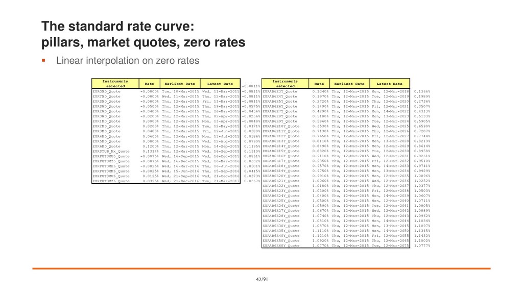
Linear interpolation on zero rates Instruments selected Rate Earliest Date Latest Date EURAB6E3Y_Quote 0.1340% Thu, 12-Mar-2015 Mon, 12-Mar-2018 0.1366% EURAB6E4Y_Quote 0.1970% Thu, 12-Mar-2015 Tue, 12-Mar-2019 0.1989% EURAB6E5Y_Quote 0.2720% Thu, 12-Mar-2015 Thu, 12-Mar-2020 0.2736% EURAB6E6Y_Quote 0.3490% Thu, 12-Mar-2015 Fri, 12-Mar-2021 0.3507% EURAB6E7Y_Quote 0.4290% Thu, 12-Mar-2015 Mon, 14-Mar-2022 0.4313% EURAB6E8Y_Quote 0.5100% Thu, 12-Mar-2015 Mon, 13-Mar-2023 0.5133% EURAB6E9Y_Quote 0.5860% Thu, 12-Mar-2015 Tue, 12-Mar-2024 0.5905% EURAB6E10Y_Quote 0.6530% Thu, 12-Mar-2015 Wed, 12-Mar-2025 0.6590% EURAB6E11Y_Quote 0.7130% Thu, 12-Mar-2015 Thu, 12-Mar-2026 0.7207% EURAB6E12Y_Quote 0.7650% Thu, 12-Mar-2015 Fri, 12-Mar-2027 0.7744% EURAB6E13Y_Quote 0.8110% Thu, 12-Mar-2015 Mon, 13-Mar-2028 0.8219% EURAB6E14Y_Quote 0.8490% Thu, 12-Mar-2015 Mon, 12-Mar-2029 0.8614% EURAB6E15Y_Quote 0.8820% Thu, 12-Mar-2015 Tue, 12-Mar-2030 0.8958% EURAB6E16Y_Quote 0.9110% Thu, 12-Mar-2015 Wed, 12-Mar-2031 0.9261% EURAB6E17Y_Quote 0.9350% Thu, 12-Mar-2015 Fri, 12-Mar-2032 0.9510% EURAB6E18Y_Quote 0.9570% Thu, 12-Mar-2015 Mon, 14-Mar-2033 0.9741% EURAB6E19Y_Quote 0.9750% Thu, 12-Mar-2015 Mon, 13-Mar-2034 0.9929% EURAB6E20Y_Quote 0.9910% Thu, 12-Mar-2015 Mon, 12-Mar-2035 1.0096% EURAB6E21Y_Quote 1.0060% Thu, 12-Mar-2015 Wed, 12-Mar-2036 1.0252% EURAB6E22Y_Quote 1.0180% Thu, 12-Mar-2015 Thu, 12-Mar-2037 1.0377% EURAB6E23Y_Quote 1.0300% Thu, 12-Mar-2015 Fri, 12-Mar-2038 1.0503% EURAB6E24Y_Quote 1.0400% Thu, 12-Mar-2015 Mon, 14-Mar-2039 1.0607% EURAB6E25Y_Quote 1.0500% Thu, 12-Mar-2015 Mon, 12-Mar-2040 1.0711% EURAB6E26Y_Quote 1.0590% Thu, 12-Mar-2015 Tue, 12-Mar-2041 1.0805% EURAB6E27Y_Quote 1.0670% Thu, 12-Mar-2015 Wed, 12-Mar-2042 1.0889% EURAB6E28Y_Quote 1.0740% Thu, 12-Mar-2015 Thu, 12-Mar-2043 1.0962% EURAB6E29Y_Quote 1.0810% Thu, 12-Mar-2015 Mon, 14-Mar-2044 1.1034% EURAB6E30Y_Quote 1.0870% Thu, 12-Mar-2015 Mon, 13-Mar-2045 1.1097% EURAB6E35Y_Quote 1.1110% Thu, 12-Mar-2015 Mon, 14-Mar-2050 1.1345% EURAB6E40Y_Quote 1.1210% Thu, 12-Mar-2015 Fri, 12-Mar-2055 1.1432% EURAB6E50Y_Quote 1.0920% Thu, 12-Mar-2015 Thu, 12-Mar-2065 1.1002% EURAB6E60Y_Quote 1.0770% Thu, 12-Mar-2015 Tue, 12-Mar-2075 1.0777% Instruments selected Rate Earliest Date Latest Date -0.0811% EUROND_Quote -0.0800% Tue, 10-Mar-2015 Wed, 11-Mar-2015 -0.0811% EURTND_Quote -0.0800% Wed, 11-Mar-2015 Thu, 12-Mar-2015 -0.0811% EURSND_Quote -0.0800% Thu, 12-Mar-2015 Fri, 13-Mar-2015 -0.0811% EURSWD_Quote -0.0500% Thu, 12-Mar-2015 Thu, 19-Mar-2015 -0.0575% EUR2WD_Quote -0.0400% Thu, 12-Mar-2015 Thu, 26-Mar-2015 -0.0456% EUR3WD_Quote -0.0200% Thu, 12-Mar-2015 Thu, 02-Apr-2015 -0.0256% EUR1MD_Quote 0.0000% Thu, 12-Mar-2015 Mon, 13-Apr-2015 -0.0048% EUR2MD_Quote 0.0200% Thu, 12-Mar-2015 Tue, 12-May-2015 0.0171% EUR3MD_Quote 0.0400% Thu, 12-Mar-2015 Fri, 12-Jun-2015 0.0380% EUR4MD_Quote 0.0600% Thu, 12-Mar-2015 Mon, 13-Jul-2015 0.0586% EUR5MD_Quote 0.0800% Thu, 12-Mar-2015 Wed, 12-Aug-2015 0.0790% EUR6MD_Quote 0.1200% Thu, 12-Mar-2015 Mon, 14-Sep-2015 0.1195% EURSTUB_Mx_Quote 0.1314% Thu, 12-Mar-2015 Wed, 16-Sep-2015 0.1310% EURFUT3MU5_Quote -0.0075% Wed, 16-Sep-2015 Wed, 16-Dec-2015 0.0861% EURFUT3MZ5_Quote -0.0075% Wed, 16-Dec-2015 Wed, 16-Mar-2016 0.0632% EURFUT3MH6_Quote -0.0025% Wed, 16-Mar-2016 Thu, 16-Jun-2016 0.0501% EURFUT3MM6_Quote -0.0025% Wed, 15-Jun-2016 Thu, 15-Sep-2016 0.0415% EURFUT3MU6_Quote 0.0125% Wed, 21-Sep-2016 Wed, 21-Dec-2016 0.0373% EURFUT3MZ6_Quote 0.0325% Wed, 21-Dec-2016 Tue, 21-Mar-2017 0.0367% 42/91

Interest Rate Curves Calibration - Basics 5. What has changed
since summer 2007

EURIBOR 6M vs EONIA SWAP 6M 44/91

BASIS SWAP 3M vs 6M - Maturity 5Y 45/91

What’s New ▪ Higher basis spreads observed on the interest
rate market since summer 2007 reflect increased credit/liquidity risk and the corresponding preference for higher frequency payments (quarterly instead of semi-annually, for instance) ▪ These large basis spreads imply that different rate curves are required for market coherent estimation of forward rates with different tenors ▪ Even sophisticated old-school bootstrapping algorithms fail to estimate correct forward Euribor rates in the new market conditions observed since the summer of 2007 46/91

The end of the 3x6 FRA textbook example (1/2) {
3M Euribor, 3x6 } != 6M Euribor 47/91

The end of the 3x6 FRA textbook example (2/2) It’s
not a correlation break 48/91

The death of the single rate curve Alternative empirical evidences
that a single curve cannot be used to estimate forward rates with different tenors: ▪ two consecutive futures are not in line with their spanning 6M FRA ▪ FRA and Futures rates are not in line with EONIA based Overnight Indexed Swaps over the same period One single curve is not enough anymore to account for forward rates of different tenor, such as 1M, 3M, 6M, 12M 49/91

Interest Rate Curves Calibration - Basics 6. Multiple forwarding rate
curves

Multiple curves In the EUR Market case, at least five
different forwarding curve are needed: ▪ EONIA ▪ 1M ▪ 3M ▪ 6M ▪ 1Y First key point: select homogeneous instruments for each forwarding curve 51/91

Overnight Curve ▪ ON, TN, SN Deposits Note: EONIA is
an average index, while ON, TN, SN are not average and do not have other fixings ▪ Spot EONIA OIS (SW, 2W, 3W, 1M, …, 12M, 15M, 18M, 21M, 2Y, …, 60Y) ▪ ECB dated EONIA OIS (from spot to about 6M) EONIA is roughly constant between ECB dates It makes sense to use piecewise constant interpolation for the first 2Y, smooth interpolation later 52/91

EONIA: piecewise constant forward 53/91

EONIA: smooth forward 54/91

EONIA curve 55/91

6M Euribor Curve Select homogeneous instruments indexed to 6M Euribor:
▪ Euribor 6M Fixing (0X6) ▪ FRAs (1X7, 2X8, …, 18X24) ▪ 6M Euribor Swaps (3Y-10Y, 12Y, 15Y, 20Y, 25Y, 30Y, 35Y, 40Y, 50Y, 60Y) ▪ 6M Euribor Fwd Swaps (15Yx45Y, 25Yx55Y) Do not use Deposits: ▪ ON, TN, SN, SW, 1M, 2M, 3M are not homogeneous ▪ 6M deposit is not in line with Euribor 6M fixing: it’s not an Euribor indexed product and it is not collateralized 56/91

Overlapping instruments 1x7, 2x8, 3x9 are overlapping with 0x6 and
6x12 in the sense that do not fix a full 6M segment: their naïve introduction leads to oscillation Classic 1x7 FRA pricing (continuous compounding): 1 × 7 = (1) (7) − 1 6 where 1 7 = − 1 ×1 − 7 ×7 = − ׬ 0 1 + ׬ 0 7 = ׬ 1 7 The 6M Euribor market does not provide direct information about 1 or,more generally, about the integral of on a rolling window not equal to 6M !!! 57/91

Synthetic deposits In order to add overlapping instruments we need
additional discount factors in the 0-6M region, i.e. “Synthetic Deposits” ▪ E.g. the 1M deposit as seen on the 6M Euribor curve First order: ▪ 6M Euribor Synthetic Deposits can be estimated using a parallel shift of the first 6M of the EONIA curve; the shift must match the observed basis between 0x6 and 6M EONIA OIS Second order: ▪ Instead of a parallel shift of the first 6M of the EONIA curve allocate the overall shift in a sloped way that fits the 6M-EONIA basis term structure slope 58/91

6M Euribor curve: pillars, quotes, discount factors 59/91

6M Euribor curve: forward rates (1/2) 0.50% 1.00% 1.50% 2.00%
2.50% 3.00% 3.50% 4.00% Jun 09 Sep 09 Dec 09 Mar 10 Jun 10 Sep 10 Dec 10 Mar 11 Jun 11 Sep 11 60/91

2.50% 3.00% 3.50% 4.00% 4.50% 5.00% 5.50% Jun 09 Dec 09 Jun 10 Dec 10 Jun 11 Dec 11 Jun 12 Dec 12 Jun 13 Dec 13 Jun 14 Dec 14 Jun 15 Dec 15 Jun 16 Dec 16 Jun 17 Dec 17 Jun 18 Dec 18 61/91

▪ Euribor 3M Fixing (0X3) ▪ Futures strip (usually 8 contracts + optional first serial) ▪ 3M Euribor Swaps (3Y-10Y, 12Y, 15Y, 20Y, 25Y, 30Y, 40Y, 50Y, 60Y) Do not use Deposits Use Synthetic Deposits (0x3 is always overlapping with Futures) 62/91

3M Euribor curve: pillars, quotes, discount factors Rate Helpers Selected
Rate Earliest Date Latest Date 1.000000000 EUR_YC3MRH_2WD 1.2183% -- Wed, 8-Jul-2009 Wed, 22-Jul-2009 0.999526446 EUR_YC3MRH_1MD 1.1196% -- Wed, 8-Jul-2009 Mon, 10-Aug-2009 0.998974782 EUR_YC3MRH_2MD 1.0607% -- Wed, 8-Jul-2009 Tue, 8-Sep-2009 0.998176561 EUR_YC3MRH_TOM3F1 1.0370% -- Thu, 9-Jul-2009 Fri, 9-Oct-2009 0.997322184 EUR_YC3MRH_FUT3MN9 1.0075% 0.0000% Wed, 15-Jul-2009 Thu, 15-Oct-2009 0.997190693 EUR_YC3MRH_FUT3MU9 0.9471% 0.0004% Wed, 16-Sep-2009 Wed, 16-Dec-2009 0.995560088 EUR_YC3MRH_FUT3MZ9 1.0562% 0.0013% Wed, 16-Dec-2009 Tue, 16-Mar-2010 0.993062730 EUR_YC3MRH_FUT3MH0 1.1600% 0.0025% Wed, 17-Mar-2010 Thu, 17-Jun-2010 0.990098576 EUR_YC3MRH_FUT3MM0 1.3985% 0.0040% Wed, 16-Jun-2010 Thu, 16-Sep-2010 0.986607501 EUR_YC3MRH_FUT3MU0 1.6766% 0.0059% Wed, 15-Sep-2010 Wed, 15-Dec-2010 0.982485576 EUR_YC3MRH_FUT3MZ0 2.0144% 0.0081% Wed, 15-Dec-2010 Tue, 15-Mar-2011 0.977637808 EUR_YC3MRH_FUT3MH1 2.2918% 0.0107% Wed, 16-Mar-2011 Thu, 16-Jun-2011 0.971887801 EUR_YC3MRH_FUT3MM1 2.5764% 0.0136% Wed, 15-Jun-2011 Thu, 15-Sep-2011 0.965595905 EUR_YC3MRH_AB3E3Y 2.0100% 0.0000% Wed, 8-Jul-2009 Mon, 9-Jul-2012 0.941842233 EUR_YC3MRH_AB3E4Y 2.3960% 0.0000% Wed, 8-Jul-2009 Mon, 8-Jul-2013 0.908914516 EUR_YC3MRH_AB3E5Y 2.6940% 0.0000% Wed, 8-Jul-2009 Tue, 8-Jul-2014 0.874012742 EUR_YC3MRH_AB3E6Y 2.9310% 0.0000% Wed, 8-Jul-2009 Wed, 8-Jul-2015 0.838338290 EUR_YC3MRH_AB3E7Y 3.1230% 0.0000% Wed, 8-Jul-2009 Fri, 8-Jul-2016 0.802666759 EUR_YC3MRH_AB3E8Y 3.2760% 0.0000% Wed, 8-Jul-2009 Mon, 10-Jul-2017 0.767698882 EUR_YC3MRH_AB3E9Y 3.4040% 0.0000% Wed, 8-Jul-2009 Mon, 9-Jul-2018 0.733707818 EUR_YC3MRH_AB3E10Y 3.5160% 0.0000% Wed, 8-Jul-2009 Mon, 8-Jul-2019 0.700381926 EUR_YC3MRH_AB3E12Y 3.7120% 0.0000% Wed, 8-Jul-2009 Thu, 8-Jul-2021 0.635311790 EUR_YC3MRH_AB3E15Y 3.9200% 0.0000% Wed, 8-Jul-2009 Mon, 8-Jul-2024 0.547174480 EUR_YC3MRH_AB3E20Y 4.0700% 0.0000% Wed, 8-Jul-2009 Mon, 9-Jul-2029 0.433077252 EUR_YC3MRH_AB3E25Y 4.0490% 0.0000% Wed, 8-Jul-2009 Mon, 10-Jul-2034 0.357872488 EUR_YC3MRH_AB3E30Y 3.9940% 0.0000% Wed, 8-Jul-2009 Fri, 8-Jul-2039 0.302130119 EUR_YC3MRH_AB3EBASIS35Y 3.9200% 0.0000% Wed, 8-Jul-2009 Fri, 8-Jul-2044 0.260893433 EUR_YC3MRH_AB3EBASIS40Y 3.8460% 0.0000% Wed, 8-Jul-2009 Thu, 8-Jul-2049 0.228482302 EUR_YC3MRH_AB3EBASIS50Y 3.7690% 0.0000% Wed, 8-Jul-2009 Tue, 8-Jul-2059 0.170286910 EUR_YC3MRH_AB3EBASIS60Y 3.7100% 0.0000% Wed, 8-Jul-2009 Mon, 8-Jul-2069 0.128986064 63/91

3M Euribor curve: forward rates (1/2) 64/91

3M Euribor curve: forward rates (1/2) 65/91

▪ Euribor 1M Fixing (0X1) ▪ Money market monthly swaps (fixed rate vs 1M Euribor, maturities ranging in 2M-12M) ▪ 1M Euribor Swaps from Basis: 1M Euribor swap rates are obtained from the same maturity 6M Euribor swap rates minus same maturity 1M/6M basis swaps (maturities 2Y-10Y, 12Y, 15Y, 20Y, 25Y, 30Y, 40Y, 50Y, 60Y) Do not use Deposits No Overlapping Instruments: no need for Synthetic Deposits but it’s possible to use them for greater curve granularity 66/91

1M Euribor curve: pillars, quotes, discount factors 67/91

1Y Euribor Curve Select homogeneous instruments indexed to 1Y Euribor:
▪ Euribor 1Y Fixing (0X12) ▪ 12x24 FRA ▪ 1Y Euribor Swaps from Basis: swap rates are obtained from the same maturity 6M Euribor swap rates plus same maturity 6M/1Y basis swaps (maturities 3Y-10Y, 12Y, 15Y, 20Y, 25Y, 30Y, 40Y, 50Y, 60Y) Do not use Deposits No Overlapping Instruments but using only 0x12 and 12x24 is too loose for market makers and results in unreliable intermediate 6x18… 70/91

Synthetic FRAs Use EONIA/1Y basis term structure to interpolate 3x15,
6x18, 9x21, 15x27, 18x30 (and 1x13, 2x14, etc) We now have Overlapping Instruments Use Synthetic Deposits 71/91

1Y Euribor curve: pillars, quotes, discount factors Rate Helpers Selected
Rate Earliest Date Latest Date 1.000000000 EUR_YC1YRH_1MD 1.9789% -- Wed, 8-Jul-2009 Mon, 10-Aug-2009 0.998189307 EUR_YC1YRH_2MD 1.8867% -- Wed, 8-Jul-2009 Tue, 8-Sep-2009 0.996761196 EUR_YC1YRH_3MD 1.7666% -- Wed, 8-Jul-2009 Thu, 8-Oct-2009 0.995505563 EUR_YC1YRH_6MD 1.5686% -- Wed, 8-Jul-2009 Fri, 8-Jan-2010 0.992046407 EUR_YC1YRH_9MD 1.4660% -- Wed, 8-Jul-2009 Thu, 8-Apr-2010 0.988965224 EUR_YC1YRH_1YD 1.4560% -- Wed, 8-Jul-2009 Thu, 8-Jul-2010 0.985452531 EUR_YC1YRH_1x13F 1.4204% -- Mon, 10-Aug-2009 Tue, 10-Aug-2010 0.984018529 EUR_YC1YRH_2x14F 1.4084% -- Tue, 8-Sep-2009 Wed, 8-Sep-2010 0.982728122 EUR_YC1YRH_3x15F 1.4228% -- Thu, 8-Oct-2009 Fri, 8-Oct-2010 0.981348597 EUR_YC1YRH_6x18F 1.5599% -- Fri, 8-Jan-2010 Mon, 10-Jan-2011 0.976517569 EUR_YC1YRH_9x21F 1.7888% -- Thu, 8-Apr-2010 Fri, 8-Apr-2011 0.971348075 EUR_YC1YRH_12x24F 2.0470% -- Thu, 8-Jul-2010 Fri, 8-Jul-2011 0.965415992 EUR_YC1YRH_15x27F 2.3231% -- Fri, 8-Oct-2010 Mon, 10-Oct-2011 0.958645347 EUR_YC1YRH_18x30F 2.5891% -- Mon, 10-Jan-2011 Tue, 10-Jan-2012 0.951538706 EUR_YC1YRH_AB12EBASIS3Y 2.2010% 0.0000% Wed, 8-Jul-2009 Mon, 9-Jul-2012 0.936394100 EUR_YC1YRH_AB12EBASIS4Y 2.5510% 0.0000% Wed, 8-Jul-2009 Mon, 8-Jul-2013 0.903300392 EUR_YC1YRH_AB12EBASIS5Y 2.8260% 0.0000% Wed, 8-Jul-2009 Tue, 8-Jul-2014 0.868336891 EUR_YC1YRH_AB12EBASIS6Y 3.0460% 0.0000% Wed, 8-Jul-2009 Wed, 8-Jul-2015 0.832722385 EUR_YC1YRH_AB12EBASIS7Y 3.2260% 0.0000% Wed, 8-Jul-2009 Fri, 8-Jul-2016 0.797122139 EUR_YC1YRH_AB12EBASIS8Y 3.3690% 0.0000% Wed, 8-Jul-2009 Mon, 10-Jul-2017 0.762304390 EUR_YC1YRH_AB12EBASIS9Y 3.4890% 0.0000% Wed, 8-Jul-2009 Mon, 9-Jul-2018 0.728491475 EUR_YC1YRH_AB12EBASIS10Y 3.5950% 0.0000% Wed, 8-Jul-2009 Mon, 8-Jul-2019 0.695315561 EUR_YC1YRH_AB12EBASIS12Y 3.7800% 0.0000% Wed, 8-Jul-2009 Thu, 8-Jul-2021 0.630749929 EUR_YC1YRH_AB12EBASIS15Y 3.9780% 0.0000% Wed, 8-Jul-2009 Mon, 8-Jul-2024 0.543211294 EUR_YC1YRH_AB12EBASIS20Y 4.1190% 0.0000% Wed, 8-Jul-2009 Mon, 9-Jul-2029 0.429818737 EUR_YC1YRH_AB12EBASIS25Y 4.0930% 0.0000% Wed, 8-Jul-2009 Mon, 10-Jul-2034 0.355049339 EUR_YC1YRH_AB12EBASIS30Y 4.0350% 0.0000% Wed, 8-Jul-2009 Fri, 8-Jul-2039 0.299587957 EUR_YC1YRH_AB12EBASIS35Y 3.9610% 0.0000% Wed, 8-Jul-2009 Fri, 8-Jul-2044 0.258213019 EUR_YC1YRH_AB12EBASIS40Y 3.8870% 0.0000% Wed, 8-Jul-2009 Thu, 8-Jul-2049 0.225739564 EUR_YC1YRH_AB12EBASIS50Y 3.8100% 0.0000% Wed, 8-Jul-2009 Tue, 8-Jul-2059 0.167657933 EUR_YC1YRH_AB12EBASIS60Y 3.7510% 0.0000% Wed, 8-Jul-2009 Mon, 8-Jul-2069 0.126593622 72/91

1Y Euribor curve: forward rates (1/2) 0.50% 1.00% 1.50% 2.00%

1Y Euribor curve: forward rates (2/2) 0.50% 1.00% 1.50% 2.00%

Curve comparison: Swaps Euribor 1M Euribor 3M Euribor 6M Euribor
1Y 3Y 0.0730% 0.1820% 0.2960% 0.4390% 4Y 0.1430% 0.2640% 0.3820% 0.5280% 5Y 0.2370% 0.3650% 0.4880% 0.6360% 6Y 0.3540% 0.4850% 0.6100% 0.7590% 7Y 0.4890% 0.6210% 0.7460% 0.8950% 8Y 0.6270% 0.7590% 0.8830% 1.0320% 9Y 0.7610% 0.8930% 1.0150% 1.1630% 10Y 0.8840% 1.0160% 1.1350% 1.2780% 12Y 1.0960% 1.2250% 1.3360% 1.4690% 15Y 1.3340% 1.4560% 1.5530% 1.6710% 20Y 1.5660% 1.6770% 1.7570% 1.8600% 25Y 1.6720% 1.7730% 1.8430% 1.9350% 30Y 1.7220% 1.8170% 1.8790% 1.9630% 40Y 1.7970% 1.8800% 1.9330% 2.0070% 50Y 1.8220% 1.8970% 1.9440% 2.0120% 60Y 1.8450% 1.9140% 1.9570% 2.0210% 75/91

Focus lens ▪ We have plotted (simple compounding) FRA rates
since this is what traders are interested in ▪ What about instantaneous (continuous compounding) forward rates? ▪ On the one day scale continuous compounding forward rates and simple compounding (i.e. ON) rates are equivalent 76/91

ON rates as seen on the 1M Euribor curve Note
the TOYs Spot Next Fwd 0.50% 1.00% 1.50% 2.00% 2.50% 3.00% 3.50% Jun 09 Sep 09 Dec 09 Mar 10 Jun 10 Sep 10 Dec 10 Mar 11 Jun 11 Sep 11 77/91

the TOYs Spot Next Fwd 0.50% 1.00% 1.50% 2.00% 2.50% 3.00% 3.50% Jun 09 Sep 09 Dec 09 Mar 10 Jun 10 Sep 10 Dec 10 Mar 11 Jun 11 Sep 11 78/91

the TOYs 79/91

Spot Next Fwd 0.50% 1.00% 1.50% 2.00% 2.50% 3.00% 3.50%
4.00% Jun 09 Sep 09 Dec 09 Mar 10 Jun 10 Sep 10 Dec 10 Mar 11 Jun 11 Sep 11 ON rates as seen on the 1Y Euribor curve No TOYs here 80/91

Interest Rate Curves Calibration – Basics 7. Discounting rate curves

Discounting curve? What do you mean/want? Two identical future cash
flows must have the same present value: we need an unique discounting curve We have bootstrapped each forwarding curve using the forwarding curve itself also for discounting swap cash flows: something is flawed here, at least when swaps are bootstrapped The discounting curve should represent the funding level implicit in whatever hedging strategy. What is the funding level? 82/91

Discounting and collateralization ▪ What are swap rates? They are
rates tradable between collateralized counterparties ▪ Capital market collateralization between two counterparties is the bilateral obligation to secure by liquid assets (such as cash or securities) the outstanding NPV of the overall trading book: these assets are called margin ▪ The margin pledged by the borrower are legally in the lender possession or subject to seizure in the event of default ▪ The collateral margin earns the overnight rate: the overnight curve is the discounting curve for collateralized transactions ▪ Using the same rationale: uncollateralized transactions should be discounted by each financial institution using its own capital market funding rates 83/91

What about counterparty credit risk? ▪ Collateralized transactions have negligible
residual credit risk: after all, that’s what collateralization was created for! ▪ Uncollateralized transactions have credit risk which must be accounted for, but this has little to do with the liquidity/funding issue 84/91

5Y Receiver Swap 2.63% 6M flat NPV evolution (Deterministic Curve)
Average NPV = -0.64%, positive cash balance: borrowing 5Y receive 2.63% pay 6M NPV% -2.50% -2.00% -1.50% -1.00% -0.50% 0.00% 0.50% 1.00% Jan 10 Jul 10 Jan 11 Jul 11 Jan 12 Jul 12 Jan 13 Jul 13 Jan 14 Jul 14 Jan 15 Jul 15 85/91

5Y receive 2.63% pay 6M-0.62% NPV% -1.00% -0.50% 0.00% 0.50%
1.00% 1.50% 2.00% 2.50% 3.00% 3.50% Jan 10 Jul 10 Jan 11 Jul 11 Jan 12 Jul 12 Jan 13 Jul 13 Jan 14 Jul 14 Jan 15 Jul 15 Asset Swap 5Y bond 2.63% 103.00 NPV evolution (Deterministic Curve) Average NPV = 1.02%, negative cash balance: lending 86/91

Forwarding and discounting rate curves: a recipe 1. Build the
EONIA curve using your preferred procedure; this is the EONIA forwarding curve and the discount curve for collateralized transactions 2. Select different sets of collateralized vanilla interest rate instruments traded on the market, each set homogeneous in the underlying Euribor rate 3. Build separated forwarding curves using the selected instruments in the bootstrapping algorithm; use the EONIA curve to exogenously discount any cashflow 87/91

The impact of exogenous EONIA discounting (1/2) Forward Euribor 88/91

The impact of exogenous EONIA discounting (2/2) Forward Swap 89/91

Interest Rate Curves Calibration - Basics 8. Bibliography

Bibliography (1/2) Ametrano, Ferdinando and Bianchetti, Marco. Everything You Always
Wanted to Know About Multiple Interest Rate Curve Bootstrapping but Were Afraid to Ask http://papers.ssrn.com/sol3/papers.cfm?abstract_id=2219548 James M. Hyman. Accurate monotonicity preserving cubic interpolation. SIAM Journal on Scientific and Statistical Computing, 1983. Piterbarg, Vladimir. Funding beyond discounting: collateral agreements and derivatives pricing. Risk Magazine February 2010 Whittall, Christopher. The price is wrong. Risk Magazine March 2010 Luigi Ballabio. “Implementing QuantLib”. http://implementingquantlib.blogspot.com/2013/10/chapter-3-part-3-of-n- bootstrapping.html 91/91

Bibliography (2/2) Mercurio, Fabio, Interest Rates and The Credit Crunch:
New Formulas and Market Models (February 5, 2009). Bloomberg Portfolio Research Paper No. 2010-01-FRONTIERS. Available at SSRN: http://ssrn.com/abstract=1332205 Morini, Massimo. Solving the Puzzle in the Interest Rate Market (October 12, 2009). Available at SSRN: http://ssrn.com/abstract=1506046 George Kirikos and David Novak. Convexity conundrums. Risk Magazine March 1997 Burghardt, Galen. The Eurodollar futures and options handbook; Irwin library of investment and finance; New York: McGraw-Hill, 2003. Burghardt, Galen and Kirshner, Susan. "One Good Turn," CME Interest Rate Products Advanced Topics. Chicago: Chicago Mercatile Exchange, 2002. Burghardt, Galen and Hoskins, William. "The Convexity Bias in Eurodollar Futures: Part 1 & 2." Derivatives Quarterly, 1995. 92/91

Rate Curves Calibration

Rate Curves Calibration

More Decks by Ferdinando M. Ametrano

Featured

Transcript