The abcd of Forward Rate Bootstrapping

Presented at the QuantLib User Meeting 2015 in Düsseldorf
http://ssrn.com/abstract=2696743

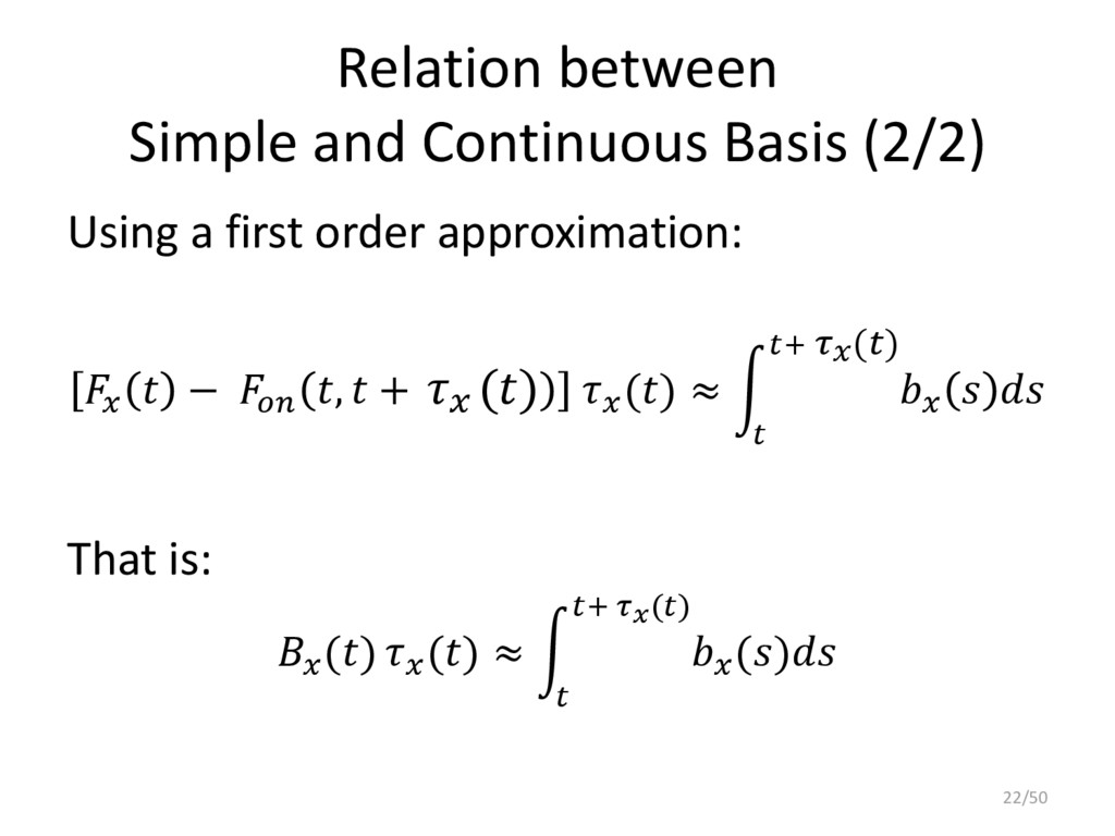
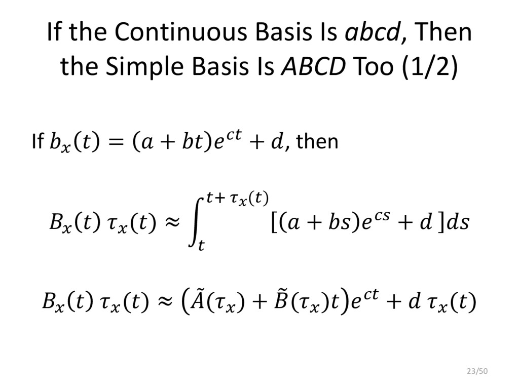
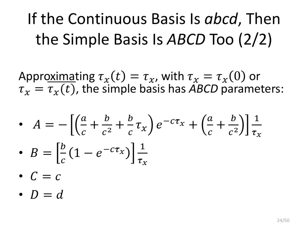
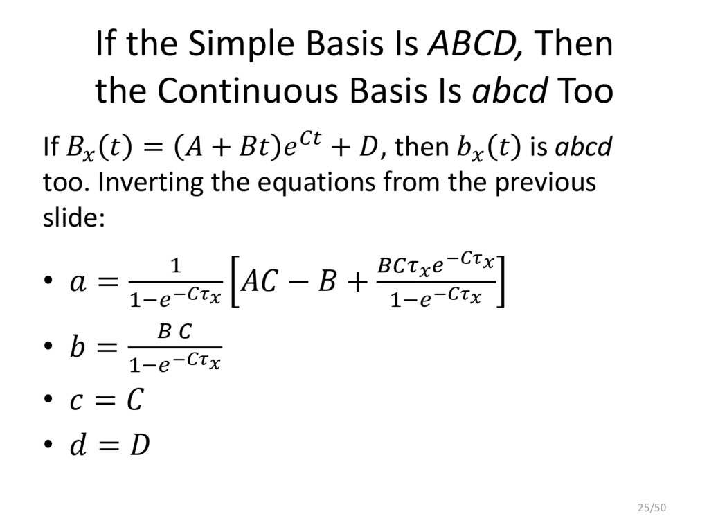
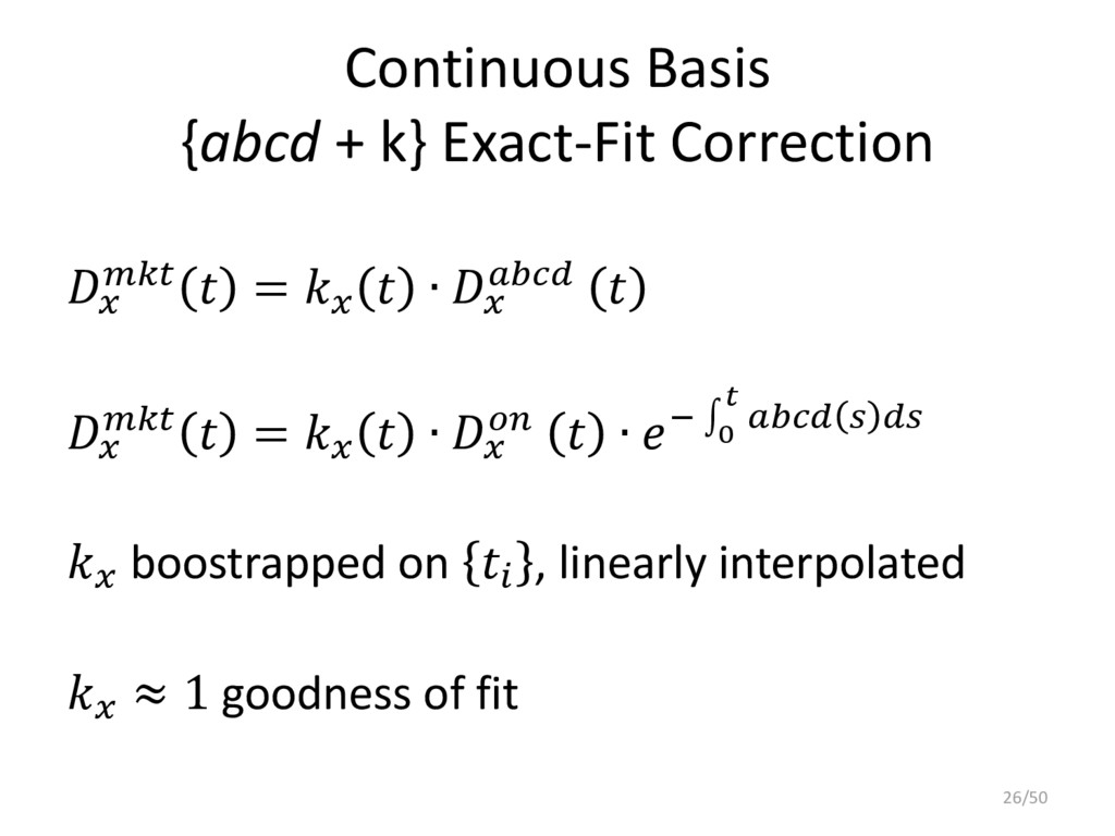
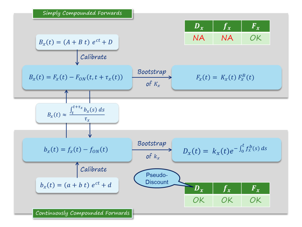
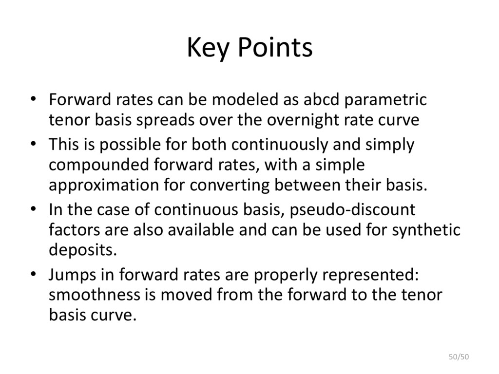
We show that forward rates can be modeled as abcd parametric tenor basis spreads over the underlying overnight rate curve. This is possible for both continuously and simply compounded forward rates, with a simple approximation for converting between the corresponding basis. In the case of continuously compounded tenor basis, pseudo-discount factors are also available for use in legacy systems. Unlike established practices, this approach properly represents the market evidence of jumps in forward rates: smoothness as quality metric is moved from the forward to the tenor basis curve.

Transcript

1. The abcd of Forward Rate Bootstrapping Ferdinando M. Ametrano ferdinando@ametrano.net Luigi Ballabio luigi.ballabio@gmail.com Paolo Mazzocchi mazzocchip@live.it https://speakerdeck.com/nando1970/the-abcd-of-forward-rate-bootstrapping http://ssrn.com/abstract=2696743 QuantLib User Meeting, Düsseldorf, November 30th 2015
2. Table of Contents 1. Pros and cons of direct forward rate bootstrapping 2. Smooth simple basis: abcd best-fit and exact-fit corrections 3. abcd parameterization of the continuous basis 4. Continuous basis in the EUR market 5. Polynomial basis and synthetic deposits 6. Conclusions 2/50
3. Forward Rates and Pseudo-Discounts 1 + () = () ( + ()) = () +() • To calculate forward rates as pseudo-discount ratio is an obsolete legacy • For a given tenor in a multi-curve world , < are not specified 3/50
4. The Problem with Pseudo-Discounts • Forward smoothness depends on discount factors of maturity below the forward tenor, e.g. for 6M 17 = 6 (1) 6 (7) = − () 1 0 − () 7 0 • Instruments of 6M tenor (e.g. 0x6, 1x7, 2x8, etc.) provide no information about 6 (1) 4/50
5. Synthetic Deposits Patch • Estimate , < to maximize forward rate smoothness = − [ +()] 0 = () ∙ − () 0 instantaneous forward rates on the ON curve () (parametric) instantaneous basis • A polynomial basis obtained as exact-fit of market instruments is suggested by Ametrano, Mazzocchi (2014) EONIA Jumps and Proper Euribor Forwarding https://speakerdeck.com/nando1970/eonia-jumps-and-proper-euribor-forwarding 5/50
6. Pseudo-Discount World: EUR6M 6/50
7. Pseudo-Discount World: EUR6M With Synthetic Deposits Patch 7/50
8. Direct Forward Rate Bootstrapping: the Problem of Non-Smooth Forwards Direct forward rate bootstrapping gets rid of the synthetic deposit problem, but • Jumps in overnight rates propagate to longer tenor ibor rates, e.g. turns of year • Additive forward rate jumps originating from the same ON jump have different magnitude for different ibor tenors • Increased jump attenuation for longer tenor, subject to convoluted estimation procedures 8/50
9. EONIA Turn of Year 9/50
10. EUR1M Turn of Year 10/50
11. EUR3M Turn of Year 11/50
12. EUR6M Turn of Year 12/50
13. The Legacy (Benchmark) EUR6M Curve • Use OIS for discounting • Never ask a forward curve for discount factors 13/50
14. EUR6M/OIS6M Simple Basis: the Empirical Observation Ibor forward rates can be seen as integral of the overnight curve plus a basis. There is no reason for this basis not to be smooth 6 = 6 − , + 6 () 14/50
15. Rebonato’s abcd Parameterization = + − + • + is the value in = 0; • is the long term value; • For a bounded (), it must be > 0; • The hump max is at: = 1 − (relevant only if positive) 15/50
16. EUR6M/OIS6M Simple Basis from ABCD FRA/Swap Calibration • A=0.1424%, B=0.001, C=0.207, D=0.0379% 16/50
17. EUR6M from Simple Basis ABCD FRA/Swap Calibration 17/50
18. Fitting to Market Instrument, Not to the Legacy Benchmark • The legacy benchmark curve is something to be improved upon, displayed as comparison • The quality of the fit has to be judged by market instruments repricing errors • Exact fit is possible with correction factors 18/50
19. EUR6M from Simple Basis {ABCD + K} Exact-Fit Correction = = + (, + ()) bootstrapped on , linearly interpolated ≈ 1 goodness of fit 19/50
20. The Case for Continuous Basis • Simple basis is observed in the market • Continuous basis is preferred for derivative pricing (Schlenkrich and Miemiec 2015) • Continuous basis also provides well defined pseudo-discounts = − [ +()] 0 = ( ) ∙ − () 0 20/50
21. Relation between Simple and Continuous Basis (1/2) • Simple basis: = − , + () • Continuous basis: = − 1 + () = () + () = +() + () = 1 + (, + ()) () () + () Therefore: ln 1 + () 1 + , + () () = () + () 21/50
22. Relation between Simple and Continuous Basis (2/2) Using a first order approximation: − , + () () ≈ + () That is: () () ≈ () + () 22/50
23. If the Continuous Basis Is abcd, Then the Simple Basis Is ABCD Too (1/2) If = + + , then () ≈ + + + () () ≈ ( ) + ( ) + () 23/50
24. If the Continuous Basis Is abcd, Then the Simple Basis Is ABCD Too (2/2) Approximating = , with = 0 or = (), the simple basis has ABCD parameters: • = − + 2 + − + + 2 1 • = 1 − − 1 • = • = 24/50
25. If the Simple Basis Is ABCD, Then the Continuous Basis Is abcd Too If = + + , then is abcd too. Inverting the equations from the previous slide: • = 1 1−− − + − 1−− • = 1−− • = • = 25/50
26. Continuous Basis {abcd + k} Exact-Fit Correction = ∙ = ∙ ∙ − 0 boostrapped on , linearly interpolated ≈ 1 goodness of fit 26/50
28. EUR6M/OIS6M Simple Basis from abcd FRA/Swap Calibration • a=0.1438%, b=0.0011, c=0.1949, d=0.0191% • A=0.1627%, B=0.0011, C=0.1949, D=0.0191% 28/50
29. EUR6M from abcd FRA/Swap Calibration 29/50
30. EUR6M abcd Errors Exact-Fit with ∈ [0.9984, 1.0005] 30/50
31. EUR3M/OIS3M Simple Basis from abcd FRA/Futures/Swap Calibration • a=0.1027%, b=0.0005, c=0.1436, d=0% • A=0.1073%, B=0.0005, C=0.1436, D=0% 31/50
32. EUR3M from abcd FRA/Futures/Swap Calibration 32/50
33. EUR3M abcd Errors Exact-Fit with ∈ [0.9980, 1.0026] 33/50
34. EUR1M/OIS1M Simple Basis from abcd Swap Calibration • a=0.0283%, b=0.0002, c=0.1958, d=0% • A=0.0291%, B=0.0002, C=0.1958, D=0% 34/50
35. EUR1M from abcd Swap Calibration 35/50
36. EUR1M abcd Errors Exact-Fit with ∈ [0.9994, 1.0020] • 36/50
37. EUR1Y/OIS1Y Simple Basis from abcd FRA/Swap Calibration • a=0.2239%, b=0.0016, c=0.2010, d=0.0406% • A=0.2741%, B=0.0016, C=0.2010, D=0.0406% 37/50
38. EUR1Y from abcd FRA/Swap Calibration 38/50
39. EUR1Y abcd Errors Exact-Fit with ∈ [0.9998, 1.0019] • 39/50
40. Synthetic Deposits: Back to the abcd Future • Synthetic deposits , < can be obtained by integration of the abcd continuous basis: = − [ +()] 0 = ( ) ∙ − () 0 • Additional recipe to the polynomial exact-fit suggestion of Ametrano, Mazzocchi (2014) 40/50
41. Synthetic Deposits: The abcd Limit • Being a global fit, abcd is often not accurate enough at the short end of the basis curve, even if { } can mitigate the issue • Key problem: lack of a liquid traded instrument for the spot tenor, e.g. 0x6 FRA 41/50
42. Polynomial Basis Parameterization at the Short End of the Curve • Ametrano, Mazzocchi (2014) used polynomials for exact-fit, but best-fit is more robust • Polynomials can be used for a best-fit focused on the basis curve short end only Continuous () = ∙ =0 Simple () = ∙ =0 42/50
43. Polynomial Basis Parameterization • Using () ≈ + () , an approximate transformation between simple and continuous polynomial basis can be obtained: () ≈ ∙ • If the simple basis is polynomial, then the continuous one is a polynomial of the same order, and vice-versa 43/50
44. Polynomial Best-fit of the Simple Basis • Best-fit is robust to left extrapolation, e.g. 0x6 FRA 44/50
45. Divide, Itera, et Impera: Polynomials Synthetic Deposits in abcd Calibration 1. Calculate the synthetic deposits using polynomial best-fit of the short end continuous basis 2. Feed these synthetic deposits (at least the 0xX FRA) in the abcd continuous basis calibration 3. Bootstrap { } 45/50
46. abcd Continuous Basis The Short End of the Curve • The integral over the first 6M is not accurate 46/50
47. abcd Continuous Basis On Polynomials Steroids • The integral over the first 6M is now accurate! 47/50
48. Further Research • Other Currencies • Delta weighted (NPV) calibration • Basis tenor dominance (1M < 3M < 6M < 1Y) 48/50
49. Bibliography • F. Ametrano, P. Mazzocchi. Eonia Jumps and Proper Euribor Forwarding (2014). https://speakerdeck.com/nando1970/eonia- jumps-and-proper-euribor-forwarding • F. Ametrano, M. Bianchetti. Everything You Always Wanted to Know About Multiple Interest Rate Curve Bootstrapping but Were Afraid to Ask (2013). http://ssrn.com/abstract=2219548 • M. Henrard. Interest Rate Modelling in the Multi-Curve Framework (Palgrave Macmillian 2014) • R. Rebonato. Volatility and Correlation (Wiley 2004) • S. Schlenkrich, A. Miemiec. Choosing the Right Spread (Wilmott 2015). http://ssrn.com/abstract=2400911 • QuantLib GitHub branch: https://github.com/paolomazzocchi/quantlib/tree/tenorbasis 49/50
50. Key Points • Forward rates can be modeled as abcd parametric tenor basis spreads over the overnight rate curve • This is possible for both continuously and simply compounded forward rates, with a simple approximation for converting between their basis. • In the case of continuous basis, pseudo-discount factors are also available and can be used for synthetic deposits. • Jumps in forward rates are properly represented: smoothness is moved from the forward to the tenor basis curve. 50/50